Abstract
Collichthys lucidus is a small fish found in offshore waters that is economically important for China. It is imperative to understand its distribution characteristics and driving factors. Based on survey data of trawl fishery resources offshore of Zhejiang province, China, in spring (April) and autumn (November) from 2018 to 2022, the spatial and temporal distributions of C. lucidus in this area were analyzed. The random forest (RF) model was used to determine the important marine factors affecting the distribution of C. lucidus. The relationship between the distributions of the important variables was analyzed. The results showed that C. lucidus was mainly distributed in coastal waters. The tail density of the species exhibited obvious seasonal variation and was significantly greater in autumn than in spring. The most important factor affecting the distribution of this species in spring and autumn was water depth. The bottom temperature, bottom salinity and dissolved oxygen concentration were also important influencing factors. The importance of these factors differed among the different seasons, while the chlorophyll a concentration and pH had no significant effect on the species distribution. This study revealed the distribution pattern of C. lucidus in offshore waters of Zhejiang Province and the influence of important marine factors on its distribution. This study can enrich the survey data on C. lucidus and provide basic data for its scientific management and protection.
Keywords:
Zhejiang offshore; Collichthys lucidus; distribution characteristics; impact factors; random forest model Key Contribution:
This study not only enriches the resource change survey data in the coastal and offshore areas but also helps to understand the response of Collichthys lucidus to environmental factors. This study provides a theoretical basis for the scientific management and effective utilization of C. lucidus species.
1. Introduction
China’s Zhejiang offshore region is located in the north-central part of the East China Sea and is an important habitat for a variety of marine organisms [1]. Due to the interactions among monsoons, the Kuroshio current and multiple water masses, such as the Yangtze River estuary diluted water, the sea area has high water temperature and a large salinity gradient. Adequate food and nutrient availability provide good breeding, feeding and overwintering conditions for fish, forming a species-rich ecosystem, which is an important area for producing offshore fishery resources in China [2]. However, due to the frequent interference of global climate change and human activities, the offshore marine environment in Zhejiang is constantly changing, as indicated by changes in temperature and frequent hypoxia in coastal waters [3]. Changes in environmental conditions have had profound impacts on the distribution of many fish and other marine organisms. Some fish may migrate to new areas to find more suitable living conditions [4,5]. This will lead to changes in fishing catches and species in the coastal waters of Zhejiang, with a series of economic impacts on fisheries and related industries.
Collichthys lucidus (Spinyhead Croaker) belongs to Perciformes, Sciaenidae and Collichthys, and is a warm-water bottom fish [6]. It is mainly distributed in the Yellow Sea, Bohai Sea, East China Sea and South China Sea in the western and central Pacific Oceans. It is the main economic fish in the coastal areas of China, Japan, North Korea, the Philippines, Indonesia and other regions [7]. The fish is rich in nutrients and has broad market prospects. It is an important fresh seafood for coastal residents and an important part of estuarine ecosystems and has good development value [8]. In offshore waters of Zhejiang Province, C. lucidus is not only used as bait for traditional fish such as Larimichthys crocea, Larimichthys polyactis and Trichiurus lepturus but is also a predator of the larvae and eggs of these economic fish. It is an important part of the marine food chain [9]. Its presence is conducive to maintaining the stability of marine ecosystems, and it plays a connecting role in marine ecosystems. In addition, C. lucidus exhibits a rapid growth rate, early sexual maturity, strong fecundity and no long-distance migratory habits. With the decline in traditional main economic fish (enemy fish), C. lucidus has been fully reproduced and grown, and the number of species have increased significantly. It has gradually become a dominant species in the northern part of Hangzhou Bay, Zhongjieshan Islands Marine Reserve and other sea areas [10,11]. The spatial activity and distribution of C. lucidus are affected by many marine factors. Understanding the spatial distribution characteristics of C. lucidus and determining the key index factors are highly important for guiding the fishing production and habitat prediction of C. lucidus.
The interaction effect of ecosystems and various environmental and biological factors on the offshore distribution of C. lucidus in the Zhejiang Province makes it difficult for the traditional generalized additive model (GAM) to reveal the dominant factors affecting the distribution of C. lucidus. The random forest (RF) model is a machine learning model based on classification and regression trees. By constructing a certain number of decision trees and combining the generated decision trees according to the corresponding criteria, an additional layer of randomness is added to reduce the influence of outliers on the prediction results. Therefore, it can be used to simulate multiple nonlinear relationships [12]. Liu [13] used the RF model and the GAM model to analyze the relationship between the catch per unit fishing effort of Euphausia superba and environmental factors, and reported that the RF model had a better fitting effect than the GAM model. Wu [14] used the RF model to analyze the influence of the marine environment on the change in spawning ground of Sepiella japonica in offshore waters of Zhejiang Province, and reported that water depth, sea surface salinity, dissolved oxygen and chlorophyll a were important driving factors. The application of a random forest model to analyze the relationships between C. lucidus and marine factors in offshore waters of Zhejiang Island allowed us to calculate the influence of each variable on the resources of C. lucidus, and it was convenient to identify the dominant factors affecting the spatial distribution of C. lucidus.
Several studies have shown that on the coast of China, C. lucidus can be divided into southern and northern populations bounded by the sea area near Zhejiang [15]. As the boundary between the two populations, the importance of Zhejiang offshore waters is self-evident. At present, the research data on the changes in C. lucidus species in Zhejiang Province are relatively old, the research area is small and the marine factors affecting these changes have not been fully recognized [16]. In addition, C. lucidus is a short-lived fish [17]. The spatial and temporal distributions of short-lived species are particularly sensitive to changes in the marine environment. Based on survey data of bottom trawl fishery resources in Zhejiang offshore waters from 2018 to 2022, this study used a random forest model to explore the spatial distribution characteristics of C. lucidus. The objective of this study was to explore the interannual variation in the spatial distribution of C. lucidus and its driving factors by using fishery survey information from this species in Zhejiang offshore waters for five consecutive years and in close real-time. The aim was to enrich the survey data of C. lucidus in coastal and offshore areas, and the scientific management and effective utilization of this species were promoted.
2. Materials and Methods
2.1. Data Source
The fisheries data were derived from the bottom trawl survey of fishery resources in offshore areas of Zhejiang Province, China. The survey times were April (spring) and November (autumn) from 2018 to 2022. The survey range was 120°30′–123°45′ E, 27°00′–30°45′ N, and included northern Zhejiang (A), central Zhejiang (B) and southern Zhejiang (C). A total of 120 stations were set up (Figure 1). The fishing vessel was named “Zhepu Fishery 43019”. The length of the vessel was 30.4 m, the width was 6.0 m and the depth was 2.7 m. The main engine power was 202 kW. The engine model of the vessel was “Weichai WP4.1Q95E41” (Weichai Power Co., Ltd., Weifang, China). A single bottom trawling method was used. According to the National “Specifications for oceanographic survey -Marine Biological Survey” (GB/T 12763.6-2007) [18], the mesh of the cod-end net was set to 25 mm, the width of the net mouth was 9.9 m and the circumference of the net mouth was 50 m. The designed average towing speed at each station was 3 kn, and the trawling time was 30 min. The samples were collected, processed and analyzed according to the National “Specifications for oceanographic survey -Marine Biological Survey” (GB/T 12763.6-2007) and “The specification for marine monitoring” (GB 17378.3-2007) [19].
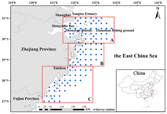
Figure 1.
Map of the bottom trawl survey area in Zhejiang Province and adjacent waters of China. A: Northern Zhejiang, B: central Zhejiang and C: southern Zhejiang. The blue dots represent the survey stations.
Bottom temperature, bottom salinity, bottom pH, chlorophyll a concentration and dissolved oxygen are known to directly influence the spawning and distribution of C. lucidus. Different water depths lead to varying changes in environmental factors such as temperature and light in the ocean, consequently impacting the ecological habits and distribution range of marine organisms [20,21]. Therefore, the variables selected in this study included the physical factor water depth (depth) and environmental factors such as bottom temperature (BST), bottom salinity (BSS), bottom dissolved oxygen (BDO), bottom chlorophyll a (BChla) and bottom pH (BpH). The above data were measured synchronously by a multifunction water quality instrument SeaBird SBE 37-SM MicroCAT (Nanjing Dongguo Marine Technology Co., Ltd., Nanjing, China).
2.2. Data Processing
This study investigated the changes in resource density of C. lucidus based on tail density. The formula for calculating the tail density of each station is as follows:
D is the mantissa density (ind/km2). C is the number of tails in the sampling area per hour (ind). q is the net capture rate, and referring to the research of Shi [22] and Yang [23], q is set to 0.5. A is the area of the net sweeping the sea per hour, which is obtained by the product of the ship speed and the sweeping width.
All of the samples were grouped according to the sampling time, and all of the stations were divided into April and November. Using R 4.0.3 software, based on the generalized linear model, the Poisson regression method was selected to evaluate the significant differences in the tail density of C. lucidus in different months.
The variance inflation factor (VIF) represents the degree of correlation between variables. The larger the VIF is, the more serious the collinearity. In general, if the VIF > 3, there is strong collinearity between variables. This should be left out before modeling [24]. Using SPSS 24.0 software, the factors with VIF less than three were selected by a multicollinearity test for subsequent analysis.
2.3. Construction and Analysis of the Random Forest Model
The random forest (RF) model is a machine learning model based on classification and regression trees [25]. It combines bagging and random feature selection to add an extra layer of randomness to bootstrap and reduce the impact of outliers on prediction results. The model has strong generalizability and is widely used in species distribution models [26]. In this study, an RF model was used to analyze the distribution and marine variables of C. lucidus. A total of 75% of the data were randomly selected from the samples as the training set for modeling, and the remaining 25% of the data were verified. Fivefold cross-validation was used to evaluate the prediction performance and accuracy of the model [27], and the calculation was repeated 100 times. According to the results of cross-validation, the number of decision trees (ntree) was set to 1000, and the number of features (mtry) was 2.
In the fitting process, to reduce the variable scale, the natural logarithm transformation of the density value Y of C. lucidus at each station was carried out. The ln (Y + 1) was obtained as the response variable. The spatial factors longitude (Lon) and latitude (Lat) and physical factor depth were selected; the environmental factors included BST, BSS, BDO, BChla, and BpH. A total of eight factors were considered explanatory variables. These factors were subsequently added to the model for fitting. According to the root mean squared error (RMSE) and mean absolute error (MAE), the difference between the predicted value and the actual value of the model was tested. The coefficient of determination R2 was used to judge the fitting degree and prediction performance of the model.
The calculation formula is as follows:
where yi represents the true value, represents the predicted value, N represents the number of true values, SSE represents the sum of squared errors and SST represents the sum of squared total deviations. Smaller RMSE and MAE values and greater R2 values indicate higher reference values of the model [28].
The calculation formula of the RF model for the importance ranking of explanatory variables is as follows:
where Vi represents the explanatory rate of the independent variable Xi to the model, SXi represents the set of nodes split by Xi under the condition of ntree, and G (Xi, v) represents the Gini information gain of Xi at the split node v.
R 4.0.3 software was used for model construction, model prediction and verification of the above steps.
2.4. Results Visualization
ArcGIS 10.1 software was used to visualize sampling sites and the distributions of C. lucidus. In order to better analyze the nonlinear relationship between tail density changes and explanatory variables, each explanatory variable was used as the X-axis, and the tail density was used as the Y-axis. Based on the “ggplot2” package in the R 4.0.3 software, locally weighted regression (LWR) was used for nonlinear fitting.
3. Results and Analysis
3.1. Changes in the Density of C. lucidus
Due to weather and other reasons, the actual number of trawl sites per year is slightly different, as detailed in Table 1. Overall, the occurrence rate of C. lucidus in spring (April) was lower than that in autumn (November). The maximum biomass density and tail density were 220.42 kg/km2 and 7.43 × 10³ ind/km2, respectively. The maximum biomass density and individual density in autumn were 611.10 kg/km2 and 25.31 × 10³ ind/km2, respectively, which were significantly greater than those in spring. By calculating the ratio of biomass density to tail density of C. lucidus at each station, the relative weight of C. lucidus individuals in spring and autumn was obtained. The results showed that the relative weight of individuals was greater in the spring.

Table 1.
Statistics on occurrence stations and resource density of C. lucidus in Zhejiang coastal waters from 2018 to 2022.
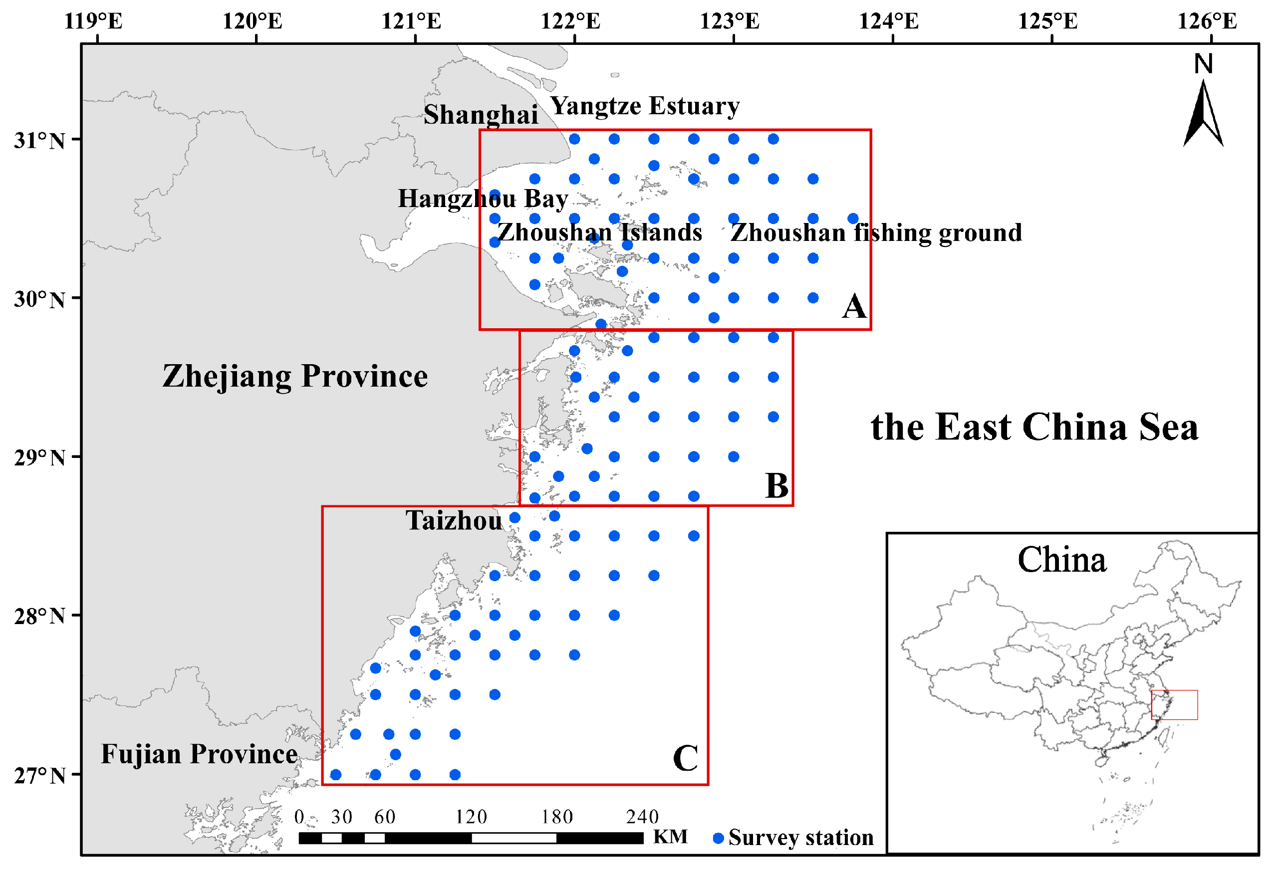
According to the annual changes, the tail density in spring and autumn showed a trend of decreasing first and then increasing (Figure 2). The tail density of C. lucidus in spring changed little among the different years and was in a stable state. The lowest average tail density, 0.29 × 10³ ind/km2, occurred in 2021. The highest value, 0.68 × 10³ ind/km2, occurred in 2022. The average tail density in autumn fluctuated greatly from year to year. The lowest value, 0.71 × 10³ ind/km2, occurred in 2020. The highest value, 2.13 × 10³ ind/km2, occurred in 2018. In addition, the tail density of C. lucidus was greater in autumn than in spring. The tail density index in autumn is 3.12 times that in spring. Poisson regression results showed that there was a significant difference in tail density between spring and autumn in 2020 (p < 0.05). Except from 2020, there were extremely significant differences in other years (p < 0.01).
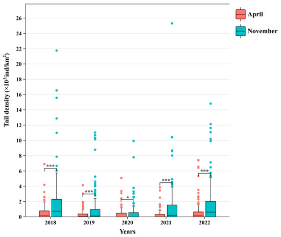
Figure 2.
Changes in tail density of C. lucidus species in spring and autumn. Red represents April, and green represents November. “*” and “***” represent the significant difference and extremely significant difference of Poisson regression, respectively.
3.2. Screening of Environmental Variables
Based on the VIF, a multicollinearity test was carried out on the six variables of depth, BST, BSS, BChla, BDO and BpH. The VIFs were all less than 3 (Table 2). Therefore, there is no multicollinearity problem between variables, which can be retained and added to the RF model for analysis.
Table 2.
Multicollinearity test of variables for the distribution of C. lucidus.
3.3. Model Performance Assessment
The fitting results of the RF model for the explanatory variables reveal that the R2 values in spring and autumn are 0.873 and 0.912, respectively, and the RMSE values are 0.180 and 0.263, respectively, indicating that the fitting effect of the model is good. The accuracy and stability of the model were tested by fivefold cross-validation. The R2 values in spring and autumn are 0.251 ± 0.054 and 0.395 ± 0.072, respectively. The standard deviation is small, indicating that the stability of the model is good. The model interpretation rates in spring and autumn are 23.26% and 34.88%, respectively (Table 3).
Table 3.
Results of model fitting and fivefold cross-validation.
3.4. Importance Ranking of Explanatory Variables
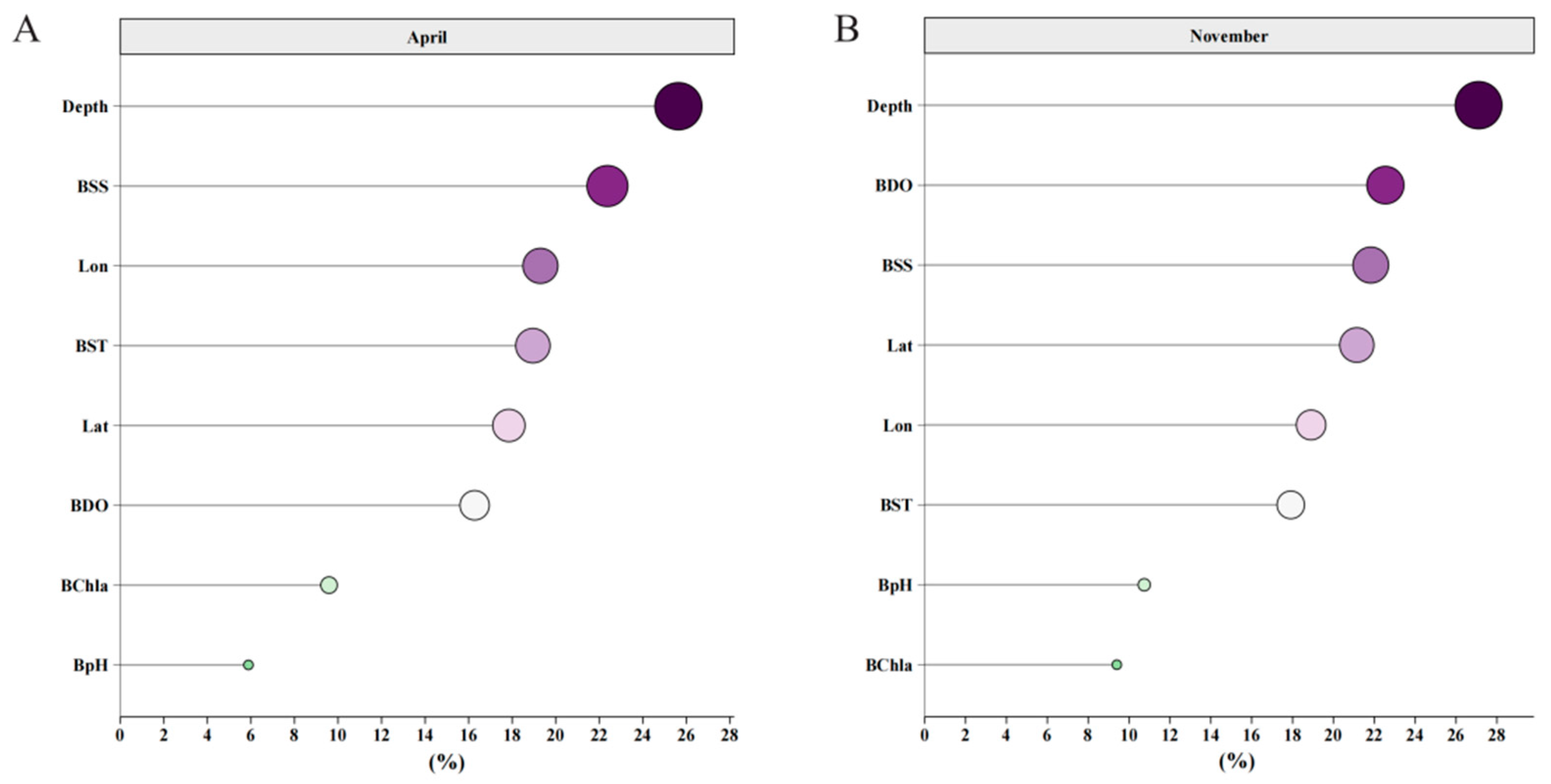
The results of the relative importance of the explanatory variables showed that the longitude and latitude of spatial factors had significant impacts on the distribution of C. lucidus species in spring and autumn. Among the marine variables, the four variables with the most influence in spring were depth, BSS, BST and BDO. The four most influential variables in autumn were depth, BDO, BSS and BST. BChla and BpH had little effect on the distribution of C. lucidus in spring or autumn, so no detailed analysis was carried out later (Figure 3).
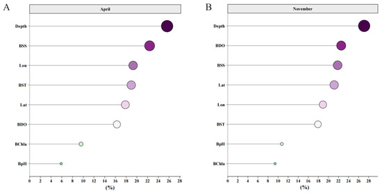
Figure 3.
The relative importance of explanatory variables for determining the distribution of C. lucidus. (A) Importance ranking of explanatory variables in April. (B) Importance ranking of explanatory variables in November. The X-axis represents the importance score of each explanatory variable, and the Y-axis represents different explanatory variables. The larger the shape of the point, the deeper the color, and the more important the variable.
3.5. The Relationships between the Distributions of C. lucidus Species and Important Explanatory Variables
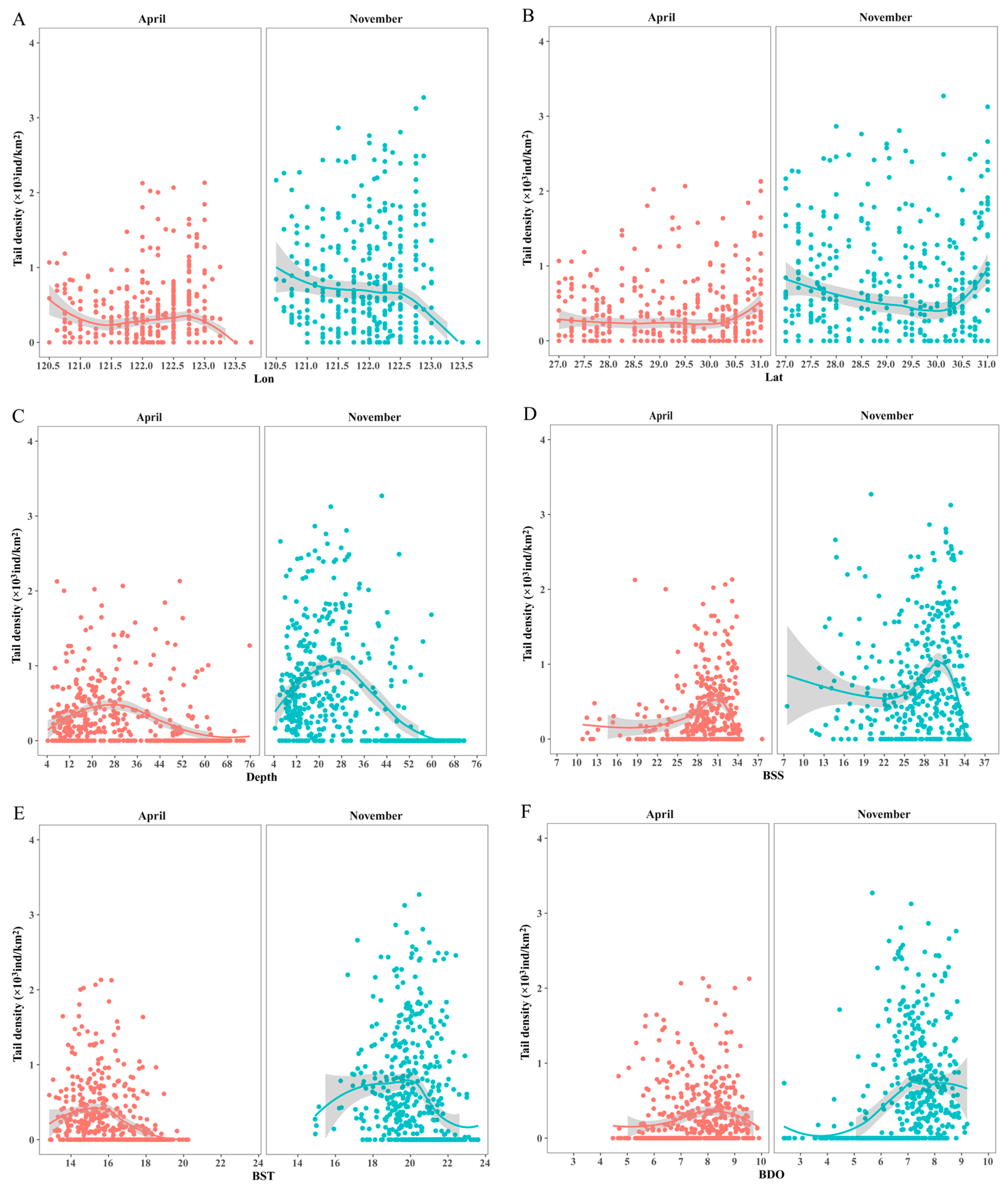
According to Figure 4, the trends of tail density in spring and autumn with different explanatory variables are nonlinear. For longitude, the optimum range in spring is between 120.5°~121° E and 122°~122° E. The change trend in autumn is small, and the resource quantity is higher within 123° E. For latitude, the change trend in spring is not obvious, and the peak value of resource is concentrated near 31° N. In autumn, the resource quantity decreases first and then increases with the increase in latitude, and the peak value is concentrated between 27°~28° N and 30.5°~31° N. For marine variables, the amount of C. lucidus in spring and autumn showed a trend of increasing first and then decreasing with the increase in depth, BSS, BST and BDO concentrations. In spring, the peak resources were mainly in the depth range of 4~30 m, the BSS range was 27~34, the BST range was 13~16 °C and the BDO range was 5~9 mg/L. In autumn, the peak resources were mainly in the depth range of 4~45 m, the BSS range was 13~34, the BST range was 17~21 °C and the BDO range was 6~9 mg/L.
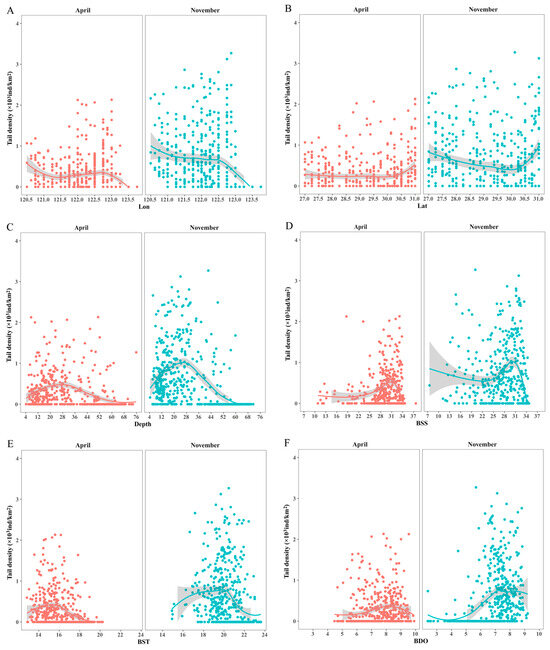
Figure 4.
The relationships between the distributions of C. lucidus species in spring and autumn and important environmental variables according to the RF model. (A) Lon; (B) lat; (C) depth; (D) BSS; (E) BST; (F) BDO. The X-axis is the range of each variable, and the Y-axis is the corresponding tail density. The curve represents the nonlinear fitting curve, and the shadow represents the confidence interval.
3.6. Spatial and Temporal Distributions of C. lucidus Species
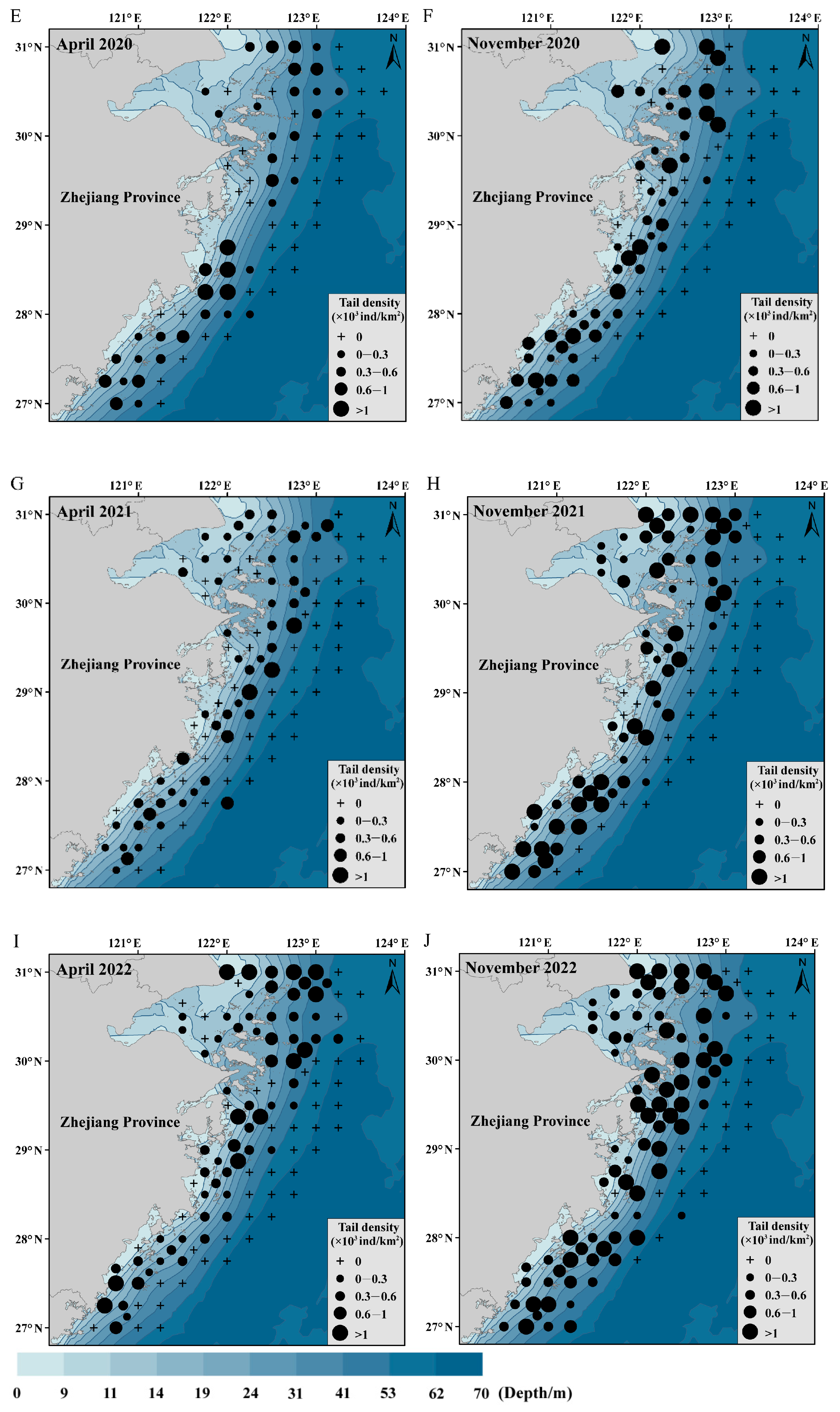
In this study, the most important explanatory variable affecting the spatial and temporal distributions of C. lucidus was water depth. Therefore, the water depth data were superimposed to construct a map of the distribution of C. lucidus species in April and November from 2018 to 2022 (Figure 5) to determine the distribution of C. lucidus in Zhejiang offshore waters, China. The distribution of the fish species is consistent with the distribution trend of the water depth contour, mainly in the northeast–southwest direction. In spring, C. lucidus was mainly distributed in the northern and central parts of Zhejiang Province and was distributed offshore and adjacent to the open seas. It was mainly distributed within 31 m of the water depth contour. The high-abundance areas were concentrated near the Yangtze estuary and Zhoushan fishing ground. In autumn, the distribution area of C. lucidus species expanded to southern Zhejiang and was distributed in the north, middle and south. It was mainly distributed within 53 m of the water depth contour. The high-abundance areas were mainly in the coastal waters.
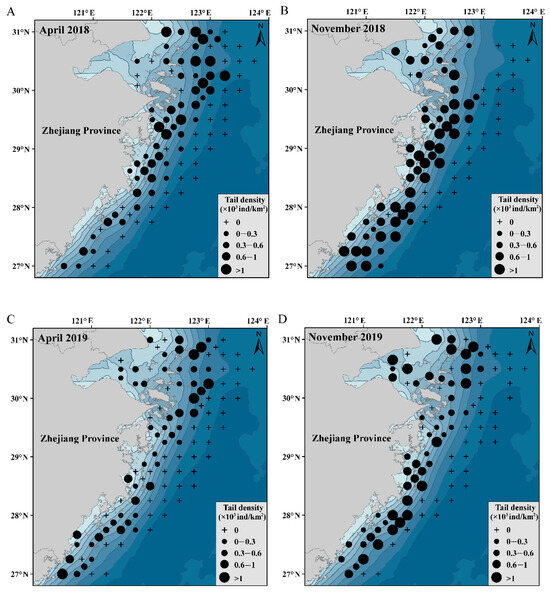
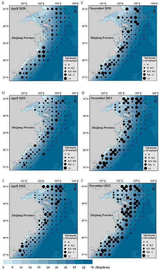
Figure 5.
The distribution of C. lucidus in spring and autumn in Zhejiang coastal waters from 2018 to 2022. (A) April 2018; (B) November 2018; (C) April 2019; (D) November 2019; (E) April 2020; (F) November 2020; (G) April 2021; (H) November 2021; (I) April 2022; (J) November 2022.
4. Discussion
4.1. Spatiotemporal Changes in the Distribution of C. lucidus
In terms of time, the distribution of C. lucidus in offshore Zhejiang changed significantly between different months and different years. The tail density of C. lucidus in April was significantly lower than that in November (Figure 2 and Figure 5). The distribution change was related to spawning, feeding and migration [29]. There are two spawning periods for C. lucidus in offshore areas of the Zhejiang Province. The spawning period in spring and summer is from late April to July. The spawning period in autumn is from September to October [30]. In spring, with increasing water temperature, the population of C. lucidus began to migrate from the deep-water area to the offshore area for feeding to prepare for life activities such as spawning and reproduction. It is speculated that the survey object of this study, which was conducted in April, was mainly spawning parents. The tail density increased significantly in November. At this time, many spawning parents had completed their breeding activities. After breeding in that year, the larvae could be captured by bottom trawling in November, which increased the tail density. It is speculated that the survey objects in November included spawning parents and supplementary groups. This also explained why the relative weight of the individuals in November was lower than that in April (Table 1). In terms of interannual variation, the tail density of C. lucidus first decreased and then decreased from 2018 to 2022. It was relatively low in 2019 and 2020 (Figure 2). The optimum bottom temperature of C. lucidus in the study area was between 17 and 21 °C in autumn, and the density was negatively correlated with the water temperature (Figure 4). According to relevant reports from the China Meteorological Administration, due to global warming, 2019 was the warmest year in which the ocean temperature was recorded [31]. The synchronous environmental data of this survey showed that the average bottom temperature in the autumn of 2019 and 2020 reached 21 °C. It is speculated that higher temperatures may affect the reproductive development of C. lucidus. In addition, the sudden outbreak of coronavirus (COVID-19) in 2019 has had a significant impact on global marine fishing [32]. During the coronavirus infection period, due to transportation restrictions and declining consumer demand, the amount of C. lucidus fishing was reduced. It is known that fishing is a key factor influencing fish resources, particularly in the short term [33], which may be the reason for the low density of C. lucidus in 2019–2020. However, the decline in industrial and daily activities during the coronavirus has also played a positive role in the recovery of marine species to a certain extent [34]. In addition to the gradual recovery of fishing activities after coronavirus, the resources have gradually increased since 2021.
Spatially, C. lucidus species were mainly distributed in the northern and central parts of Zhejiang in spring and in the northern, central and southern parts of Zhejiang offshore regions in autumn. C. lucidus is a low-grade carnivorous fish of which plankton are the main food. The food composition includes Acetes chinensis, Myctophum pterotum and Calanus sinicus. The frequency and abundance of most food species were greater in autumn than in spring. These species are distributed mainly along offshore coasts and near islands and reefs [35]. Studies have reported that the abundance of fish species is closely related to the abundance of bait, and the abundant food resources in the sea area are an important reason for fish aggregation [36,37]. In autumn, most of the spawning parents began to feed, and the supplementary group began to fatten. The abundant food in the coastal waters caused C. lucidus to gather there. In the same year, the supplementary group of juvenile fish bred in shallow waters moved offshore to southern Zhejiang so that the species were distributed in the north, middle and south of the offshore region in autumn. In addition, the difference in the spatial distribution of C. lucidus may be related to climate. The northern and central parts of Zhejiang Province are temperate sea areas, and the southern part of Zhejiang belongs to the subtropical sea area. Due to the influence of the Taiwan warm current, the Kuroshio warm current and its branches, the water temperature in the southern part of the country is higher [38]. These regional differences in climate and environmental conditions may lead to differences in the distributions of C. lucidus in the north and south. Many studies have shown that the genetic diversity of C. lucidus is high. In China’s coastal areas, the population is clearly divided into northern and southern populations near Taizhou, Zhejiang Province. There are obvious differences in gene exchange and habitat utilization patterns [39,40]. It is speculated that most of the C. lucidus in northern and central Zhejiang in this study were northern, whereas most of them in southern Zhejiang were southern. This phenomenon of north–south differentiation may also explain the spatial difference in the distribution.
4.2. Effects of Marine Variables on the Distribution of C. lucidus Species
The distribution of C. lucidus is not only affected by the reproductive habits of parents but also closely related to the marine environment. The results of relative importance showed that the most important factor affecting the distribution of C. lucidus in spring and autumn was water depth (Figure 3). Water depth can not only reflect changes in pressure and light intensity but also lead to changes in physical and chemical factors such as water temperature and salinity [41]. The model fitting results and the distribution map (Figure 4 and Figure 5) showed that the tail density of C. lucidus was the highest near a water depth of 28~30 m in spring. A high tail density in autumn occurred in the shallow water area near a water depth of 40 m. This occurred because April was the main spawning month for C. lucidus, while November was the supplementary population month and a small number of parents spawned in autumn. The suitable habitat depths of fish individuals at different developmental stages are different [42].
In addition to water depth, environmental factors such as bottom salinity, bottom temperature and dissolved oxygen also have important influences on the distribution of C. lucidus. Salinity can affect the survival rate of fish eggs and juveniles through osmotic pressure, which plays an important role in the growth and development of fish [43]. The results of the RF model showed that the suitable salinity range for C. lucidus in spring was between 27 and 34. The suitable salinity range in autumn was wide, ranging between 13 and 34 (Figure 4). Many studies have shown the characteristics of C. lucidus tolerance to a wide range of salinities [44], but Liu [45] reported that the buoyancy of fish eggs and the development of juveniles are closely related to the salinity of the habitat. A high-salinity water environment is often needed to stimulate parent spawning, reproduction and early juvenile growth. Compared with November, bottom salinity had a greater impact on the distribution of C. lucidus in April. In April, most C. lucidus plans began or were ready to enter the life stage of spawning and reproduction, which may be the main reason why C. lucidus often appears in high-salinity waters.
Seawater temperature can not only affect the reproduction and development of fish, but also change the distribution and quantity of bait, which indirectly affects the migration and distribution of fish [46]. This study revealed that the suitable temperatures for C. lucidus in offshore waters of Zhejiang Province in spring and autumn were 13~16 °C and 17~21 °C, respectively (Figure 4). Compared with the suitable temperature range for C. lucidus in the Pearl River estuary of China [20], these values were slightly lower. This difference may be related to the large scale of water temperature changes and the difference in investigation times between different sea areas. Moreover, studies have confirmed that the C. lucidus strains in the offshore region of Zhejiang and the Pearl River estuary belong to different populations [37], and there may be some differences in their adaptability to seawater temperature. In addition, the bottom water temperature had a greater impact on the distribution of C. lucidus species in spring. This difference may be related to the combined action of multiple water masses and ocean currents in offshore regions of Zhejiang. In spring, the coastal current in the Zhejiang offshore region gradually increased, and the offshore region exhibited low-temperature characteristics, while the fish were mainly spawning parents. Changes in water temperature strongly influence the gonadal development of C. lucidus, so this species is more sensitive to the changes in water temperature. In autumn, affected by the Taiwan warm current and the Kuroshio warm current, the water temperature and salinity in offshore regions of Zhejiang could be maintained at their levels. This approach can provide the necessary environmental conditions for the growth of juvenile fish, thereby reducing the impact of water temperature changes on the distribution of fish species.
Dissolved oxygen is one of the most basic parameters of oceanography. Its concentration difference affects the classification and size of plankton communities, which in turn affects a series of ecological activities in fish [47]. Usually, most fish prefer to live in habitats with high concentrations of dissolved oxygen [48]. In recent years, due to human activities, a large amount of nutrients and industrial wastewater have been transported to estuaries and coastal waters. This leads to the aggravation of eutrophication in offshore waters and a decrease in the dissolved oxygen concentration [49]. In the offshore region of Zhejiang, especially in the Yangtze River estuary and adjacent waters, hypoxia is more common [50], which affects fishery production, community structure and the ecological stability of the sea area. In the present study, the suitable dissolved oxygen concentration range for C. lucidus was 5~9 mg/L. The highest tail density in spring was nearly 7 mg/L, and that in autumn was nearly 6 mg/L. It is speculated that C. lucidus is a kind of fish that can adapt to low-oxygen environments. C. lucidus has a large gill area, abundant hemoglobin, and high water content in their muscle [51]. These physiological characteristics can increase the absorption and transport efficiency of oxygen. The same volume of fish can dissolve more oxygen, thereby reducing the demand for dissolved oxygen. Some low-oxygen-tolerant organisms can use low-oxygen waters to evade natural enemies [52]. In shallow offshore areas with low dissolved oxygen concentrations, some predators and competitors of C. lucidus may be excluded, which is also the reason why C. lucidus density is greater under lower dissolved oxygen conditions.
5. Conclusions
Surveying revealed that the distribution of C. lucidus in offshore regions of Zhejiang, China, varied greatly during different seasons. In spring, it is mainly distributed in the northern and central Zhejiang Sea areas. In autumn, the species is distributed in offshore waters in the north, middle and south of Zhejiang. In this study, the random forest model was used to screen the important driving factors influencing the distribution of C. lucidus species, and the relationships between them were fitted and analyzed. Compared with the traditional linear regression model, the RF model has the characteristics of ensemble learning. By constructing many different regression trees to improve the accuracy of the results, the generalization ability of the model is strengthened, and the fitting effect is good. However, the RF model may also exhibit overfitting [53]. Understanding the relationship between species distribution characteristics and the environment is the premise of rational utilization and scientific management. This study revealed that different variables have different effects on the distribution of C. lucidus in spring and autumn, suggesting that the species have different levels of adaptability to habitat environments at different developmental stages. Water depth, bottom salinity, bottom temperature and bottom dissolved oxygen have important effects in spring and autumn. Due to the reasons of data acquisition, this study analyzed the influence of only water depth, bottom temperature, bottom salinity, bottom dissolved oxygen, bottom chlorophyll a and bottom pH on the distribution of C. lucidus. However, the distribution of food organisms, ocean currents and other factors are also important factors affecting the spatial and temporal distributions of fish. With the continuous improvement in data acquisition, important environmental and biological factors will be introduced into the model to further improve the fitting and prediction accuracy of the model.
Author Contributions
W.X., methodology, formal analysis and writing—original draft preparation. H.Z. (Hongliang Zhang), data curation. H.Z. (Haobo Zhang) and T.W., software analysis. Y.Z., supervision and project administration. W.Z., writing—review and editing, visualization, supervision and project administration. All authors have read and agreed to the published version of the manuscript.
Funding
This study was funded by the Key Technology and System Exploration of Quota Fishing, Ministry of Agriculture and Rural Affairs, Fishery Management Fund Project [Grant number: 36, 2017], and the Zhejiang Fishery Resources Survey Special Project [HYS-CZ-202314].
Institutional Review Board Statement
Not applicable.
Data Availability Statement
The datasets that support the findings of this study are available from the corresponding author upon reasonable request.
Acknowledgments
We thank the staff of Zhejiang Marine Fisheries Research Institute for their help and support in our experiment.
Conflicts of Interest
All authors declare no conflicts of interest.
References
- Zhao, S.L.; Xu, H.X.; Zhong, J.S.; Chen, J. Zhejiang Marine Fishes; Zhejiang Science and Technology Press: Hangzhou, China, 2016; pp. 86–92. [Google Scholar]
- Zhu, Y.D.; Zhang, C.L.; Cheng, Q.T. Fishes of East China Sea; Science Press: Beijing, China, 1963; pp. 241–243. [Google Scholar]
- Zhou, F.; Qian, Z.Y.; Liu, A.Q.; Ma, X.; Ni, X.B.; Zeng, D.Y. Recent progress on the studies of the physical mechanisms of hypoxia off the Changjiang (Yangtze River) Estuary. J. Mar. Sci. 2021, 39, 22–38. [Google Scholar] [CrossRef]
- Gao, F.; Chen, X.J.; Guan, W.J.; Li, G. A New model to forecast fishing ground of Scomber japonicus in the Yellow Sea and East China Sea. Acta Oceanol. Sin. 2016, 35, 74–81. [Google Scholar] [CrossRef]
- Hu, W.J.; Du, J.G.; Su, S.K.; Tan, H.J.; Yang, W.; Ding, L.K.; Dong, P.; Yu, W.W.; Zheng, X.Q.; Chen, B. Effects of climate change in the seas of China: Predicted changes in the distribution of fish species and diversity. Ecol. Indic. 2022, 134, 108489. [Google Scholar] [CrossRef]
- Ji, Q.; Xie, Z.L.; Gan, W.; Wang, L.M.; Song, W. Identification and Characterization of PIWI-Interacting RNAs in Spinyhead Croakers (Collichthys lucidus) by Small RNA Sequencing. Fishes 2022, 7, 297. [Google Scholar] [CrossRef]
- Song, W.; Gan, W.; Xie, Z.L.; Chen, J.; Wang, L.M. Small RNA sequencing reveals sex-related miRNAs in Collichthys lucidus. Front. Genet. 2022, 13, 955645. [Google Scholar] [CrossRef]
- Ou, Y.J.; Liao, R.; Li, J.E.; Gou, X.W. Studies on the spawning period and growth of Collichthys lucidus in estuary of Pearl River based on otolith daily annulus. J. Oceanogr. Taiwan Strait. 2012, 31, 85–88. [Google Scholar] [CrossRef]
- Zhang, H.Y.; Lin, L.S. Spatial heterogeneity of Trichiurus japonicus and small-scale fish in East China Sea and their spatial relationships. Chin. J. Appl. Ecol. 2005, 16, 708–711. [Google Scholar] [CrossRef]
- Wang, M.; Hong, B.; Zhang, Y.P.; Sun, Z.Z. Spring and summer fish community structure in northern Hangzhou bay. J. Hydrol. 2016, 37, 75–81. [Google Scholar] [CrossRef]
- Zhang, H.L.; Wang, Y.; Liang, J.; He, Z.T.; Zhou, Y.D. Seasonal Variations of the Biological Characteristics and Abundance Density of Collichthys lucidus in Zhongjieshan Islands Marine Protected Area. J. Zhejiang Ocean Univ. Nat. Sci. 2015, 34, 407–410. [Google Scholar]
- DeLuca, N.M.; Mullikin, A.; Brumm, P.; Rappold, A.G.; Hubal, E.C. Using Geospatial Data and Random Forest To Predict PFAS Contamination in Fish Tissue in the Columbia River Basin, United States. Environ. Sci. Technol. 2023, 57, 14024–14035. [Google Scholar] [CrossRef] [PubMed]
- Liu, J.C.; Jia, M.X.; Feng, W.D.; Liu, C.D.; Huang, L.Y. Spatial-temporal distribution of Antarctic Krill (Euphausia superba)resource and its association with environment factors revealed with RF and GAM Models. J. Ocean Univ. China 2021, 51, 20–29. [Google Scholar] [CrossRef]
- Wu, T.; Liang, J.; Zhou, Y.D.; Xuan, W.D.; Fang, G.J.; Zhang, Y.Z.; Chen, F. The factors driving the spatial variation in the selection of spawning grounds for Sepiella japonica in offshore Zhejiang Province, China. Fishes 2024, 9, 20. [Google Scholar] [CrossRef]
- Zhang, S.; Li, M.; Yan, S.; Kong, X.l.; Zhu, J.F.; Xu, S.N.; Chen, Z.Z. Population genetic structure analysis of big head croaker (Collichthys lucidus) based on mitochondrial cytochrome b gene sequences. J. Fish. Sci. China 2021, 28, 90–99. [Google Scholar] [CrossRef]
- Wu, C.W.; Wang, W.H. Distribution biology and resource changes of Collichthys lucidus in Zhejiang coastal waters. Marine Fish. 1991, 13, 6–10. [Google Scholar]
- Wu, Z.X.; Wu, C.W.; Wang, W.H.; Hu, N.Q. Growth law of Collichthys lucidus in Zhejiang offshore research on group composition. Fish. Sci. Technol. Inf. 1990, 6, 170–174. [Google Scholar] [CrossRef]
- GB/T 12763.6-2007; Specifications for Oceanographic Survey-Part 6: Marine Biological Survey. General Administration of Quality Supervision, Inspection and Quarantine of the People’s Republic of China: Beijing, China, 2007.
- GB/T 17378.3-2007; The Specification for Marine Monitoring-Part 3: Sample Collection, Storage and Transportation. General Administration of Quality Supervision, Inspection and Quarantine of the People’s Republic of China: Beijing, China, 2007.
- Xiong, P.L.; Xu, S.N.; Chen, Z.Z.; Zhang, S.; Jiang, P.W.; Fan, J.T. Spatiotemporal distribution of Collichthy lucidus in the Pearl River Estuary and its relationship with environmental factors. Mar. Sci. 2022, 46, 79–87. [Google Scholar] [CrossRef]
- Zou, M.X.; Chen, Y.G.; Song, X.J.; Li, S.F.; Zhong, J.S. Distribution and drift trend of Collichthys lucidus larvae and juveniles in the coastal waters of the southern Yellow Sea. J. Fish. China 2022, 46, 557–568. [Google Scholar] [CrossRef]
- Shi, Y.R.; Chao, M.; Quan, W.M.; Tang, F.H.; Shen, X.Q.; Yuan, Q.; Huang, H.J. Spatial variation in fish community of Yangtze River estuary in spring. J. Fish. China 2011, 18, 1141–1151. [Google Scholar] [CrossRef]
- Yang, C.H.; Li, X.D.; Yang, Q.; Wang, Y.B. Application of machine learning methods for estimating the biomass of economically important crabs in the Zhoushan fishery. Mar. Sci. 2023, 47, 61–70. [Google Scholar] [CrossRef]
- Gómez, S.R.; Sánchez, R.A.; García, G.C.; Pérez, J.G. The VIF and MSE in Raise Regression. Mathematics 2020, 8, 605. [Google Scholar] [CrossRef]
- Flores, A.; Wiff, R.; Donovan, C.; Gálvez, P. Applying machine learning to predict reproductive condition in fish. Ecol. Inform. 2024, 80, 102481. [Google Scholar] [CrossRef]
- Rahman, L.F.; Marufuzzaman, M.; Alam, L.; Bari, M.A.; Sumaila, U.R.; Sidek, L.M. Application of Machine Learning to Investigate the Impact of Climatic Variables on Marine FishLandings. Natl. Acad. Sci. Lett. 2022, 45, 245–248. [Google Scholar] [CrossRef]
- Kang, H.; Jeon, D.J.; Kim, D.; Jung, K. Estimation of fish assessment index based on ensemble artificial neural network for aquatic ecosystem in South Korea. Ecol. Indic. 2022, 136, 108708. [Google Scholar] [CrossRef]
- Xu, B.D.; Zhang, C.L.; Xue, Y. Optimization of sampling effort for a fishery-independent survey with multiple goals. Environ. Monit. Assess. 2015, 187, 252. [Google Scholar] [CrossRef]
- Hitomi, O.; Satoshi, S.; Daisuke, A. Modeling the growth, transport, and feeding migration of age-0 Pacific saury Cololabis saira. Fish Sci. 2022, 88, 131–147. [Google Scholar]
- Wang, M.; Xu, K.D.; Liang, J. Preliminary analysis of biological characteristics of reproductive stocks of Collichthys lucidus in Northern Hangzhou Bay. J. Ocean Univ. Shanghai 2018, 27, 781–788. [Google Scholar] [CrossRef]
- Wang, Y.L.; Wang, J.; Zhou, Y.D.; Xu, K.D.; Jiang, R.J.; Li, Z.H.; Zhu, H.C.; Wang, J.; Cui, G.C. Spatial and temporal distribution characteristics of Larimichthys polyactis in Zhoushan fishing ground and the adjacent waters based on two-stage GAM. Fish. J. Fish. China 2022, 29, 633–641. [Google Scholar] [CrossRef]
- Papcunová, V.; Gregáňová, R.H. Global Impacts of COVID-19 on the Financing of Local Self-Governments: Evidence from Slovak municipalities. SHS Web Conf. 2021, 92, 01038. [Google Scholar] [CrossRef]
- Jackson, J.B.; Kirby, M.X.; Berger, W.H.; Bjorndal, K.A.; Botsford, L.W.; Bourque, B.J.; Bradbury, R.; Cooke, R.G.; Erlandson, J.M.; Estes, J.A.; et al. Historical overfishing and the recent collapse of coastal ecosystems. Science 2001, 293, 629–637. [Google Scholar] [CrossRef]
- Al Shehhi, M.R.; Samad, Y.A. Effects of the Covid-19 pandemic on the oceans. Remote Sens. Lett. 2021, 12, 325–334. [Google Scholar] [CrossRef]
- He, Z.T.; Zhang, Y.Z.; Xue, L.J.; Jin, H.W.; Zhou, Y.D. Seasonal and ontogenetic diet composition variation of Collichthys lucidus in inshore waters in the north of East China Sea. Mar. Fish. 2012, 34, 270–276. [Google Scholar] [CrossRef]
- Pothoven, A.S. The influence of ontogeny and prey abundance on feeding ecology of age-0 Lake Whitefish (Coregonus clupeaformis) in southeastern Lake Michigan. Ecol. Freshw. Fish 2020, 29, 103–111. [Google Scholar] [CrossRef]
- Sun, X.H.; Song, M.P.; Li, Z.G.; Song, Y.; Yuan, X.N.; Dong, B.; Zhang, L.; Zhu, L.X.; Liang, Z.L. Selective feeding of the mullet larvae Liza haematocheila during ontogeny in Laizhou Bay, Bohai Sea, China: The importance of small copepods in mesozooplankton as prey. Front. Mar. Sci. 2023, 10, 1147886. [Google Scholar] [CrossRef]
- Cai, R.S.; Chen, J.L.; Huang, R.H. The response of marine environment in the offshore area of China and its adjacent ocean to recent global climate change. Chin. J. Atmos. Sci. 2006, 30, 1019–1033. [Google Scholar]
- Xiao, J.Z.; Zou, Y.; Xiao, S.J.; Chen, J.N.; Wang, Z.Y.; Wang, Y.L.; Jie, X.M.; Cai, Y.M. Development of a PCR-based genetic sex identification method in spinyhead croaker (Collichthys lucidus). Aquac. Rep. 2020, 522, 735130. [Google Scholar] [CrossRef]
- Song, N.; Ma, G.Q.; Zhang, X.M.; Gao, T.X.; Sun, D.R. Genetic structure and historical demography of Collichthys lucidus inferred from mtDNA sequence analysis. Environ. Biol. Fish. 2014, 97, 69–77. [Google Scholar] [CrossRef]
- Francis, M.P.; Hurst, R.J.; McArdle, B.H.; Bagley, N.W.; Anderson, O.F. New Zealand demersal fish assemblages. Environ. Biol. Fish. 2002, 65, 215–234. [Google Scholar] [CrossRef]
- Jiang, R.J.; Sun, H.Q.; Li, X.F.; Zhou, Y.D.; Chen, F.; Xu, K.D.; Li, P.F.; Zhang, H.L. Habitat suitability evaluation of Harpadon nehereus in nearshore of Zhejiang province, China. Front. Mar. Sci. 2022, 9, 961735. [Google Scholar] [CrossRef]
- Bhat, M.; Nayak, V.N.; Chandran, M.D.S.; Ramachandra, T.V. Fish distribution dynamics in the Aghanashini estuary of Uttara Kannada, west coast of India. Curr. Sci. India 2014, 106, 1739–1744. [Google Scholar] [CrossRef]
- Zhang, S.; Jiang, Y.E.; Li, M.; Zhu, J.F.; Xu, S.N.; Chen, Z.Z. Life history of spinyhead croaker Collichthys lucidus (Sciaenidae) differentiated among populations from Chinese coastal waters. Aquat. Biol. 2022, 31, 65–76. [Google Scholar] [CrossRef]
- Liu, H.B.; Jiang, T.; Huang, H.H.; Shen, X.Q.; Zhu, J.B.; Yang, J. Estuarine dependency in Collichthys lucidus of the Yangtze River Estuary as revealed by the environmental signature of otolith strontium and calcium. Environ. Biol. Fish. 2015, 98, 165–172. [Google Scholar] [CrossRef]
- Lewin, W.C.; Mehner, T.; Ritterbusch, D.; Brämick, U. The influence of anthropogenic shoreline changes on the littoral abundance of fish species in German lowland lakes varying in depth as determined by boosted regression trees. Hydrobiologia 2014, 724, 293–306. [Google Scholar] [CrossRef]
- Rabalais, N.N.; Diaz, R.J.; Levin, L.A.; Turner, R.E.; Gilbert, D.; Zhang, J. Dynamics and distribution of natural and human-caused hypoxia. Biogeosciences 2010, 7, 585–619. [Google Scholar] [CrossRef]
- Maes, J.; Stevens, M.; Breine, J. Modelling the migration opportunities of diadromous fish species along a gradient of dissolved oxygen concentration in a European tidal watershed. Estuar. Coast. Shelf Sci. 2007, 75, 151–162. [Google Scholar] [CrossRef]
- Rabalais, N.N.; Cai, W.J.; Carstensen, J.; Conley, D.J.; Fry, B.; Hu, X.P.; Quiñones-Rivera, Z.; Rosenberg, R.; Slomp, C.P.; Turner, R.E.; et al. Eutrophication-Driven deoxygenation in the coastal ocean. Oceanography 2014, 27, 172–183. [Google Scholar] [CrossRef]
- Wang, H.J.; Dai, M.H.; Liu, J.W.; Kao, S.J.; Zhang, C.; Cai, W.J.; Wang, G.Z.; Qian, W.; Zhao, M.X.; Sun, Z.Y. Eutrophication-Driven hypoxia in the East China Sea off the Changjiang Estuary. Environ. Sci. Technol. 2016, 50, 2255–2263. [Google Scholar] [CrossRef]
- Zhang, Y. Analysis and evaluation of nutritional component in muscle of Collichthys lucidus. Sci. Fish Farming 2022, 43, 75–76. [Google Scholar] [CrossRef]
- Sato, K.N.; Levin, L.A.; Schiff, K. Habitat compression and expansion of sea urchins in response to changing climate conditions on the California continental shelf and slope (1994–2013). Deep Sea Res. Part II 2017, 137, 377–389. [Google Scholar] [CrossRef]
- Culter, D.R.; Edwards, T.C.; Beard, K.H.; Hess, K.T. Random forests for classification in ecology. Ecology 2007, 88, 2783–2792. [Google Scholar] [CrossRef]

Disclaimer/Publisher’s Note: The statements, opinions and data contained in all publications are solely those of the individual author(s) and contributor(s) and not of MDPI and/or the editor(s). MDPI and/or the editor(s) disclaim responsibility for any injury to people or property resulting from any ideas, methods, instructions or products referred to in the content. |
© 2024 by the authors. Licensee MDPI, Basel, Switzerland. This article is an open access article distributed under the terms and conditions of the Creative Commons Attribution (CC BY) license (https://creativecommons.org/licenses/by/4.0/).