4.1. Overview
Since existing distance learning approaches are mainly designed for the enhanced performance of generic distance classifiers such as KNN, SVM, etc., there are no specific constraints applied to either classifier complexity, training size, or employed representation. Conversely, there are restrictions that apply when designing distance metrics for signature-based bio-cryptography. For instance, these systems involve a simple thresholding distance classifier which makes it hard to model complex problems like offline signature verification (OLSV). Moreover, OLSV systems should learn from limited positive signature samples and almost no forgeries are available during the design phase. Lastly, the design of such systems requires concise feature representations which might not capable of alleviating the high variability in the signature images. These design constraints require a specialized distance learning method for the problem at hand.
In this paper, the distance metric defined by Equation (
4) is optimized based on a mixture of Feature-Distance (FD) space [
28,
29] and dissimilarity matrix analysis.
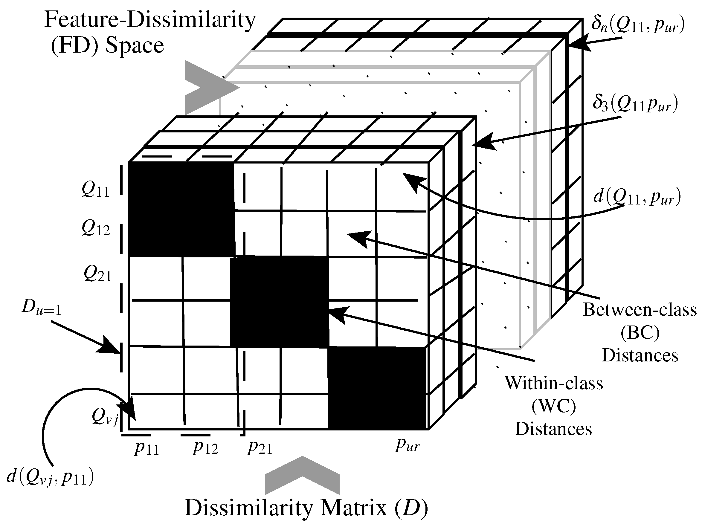
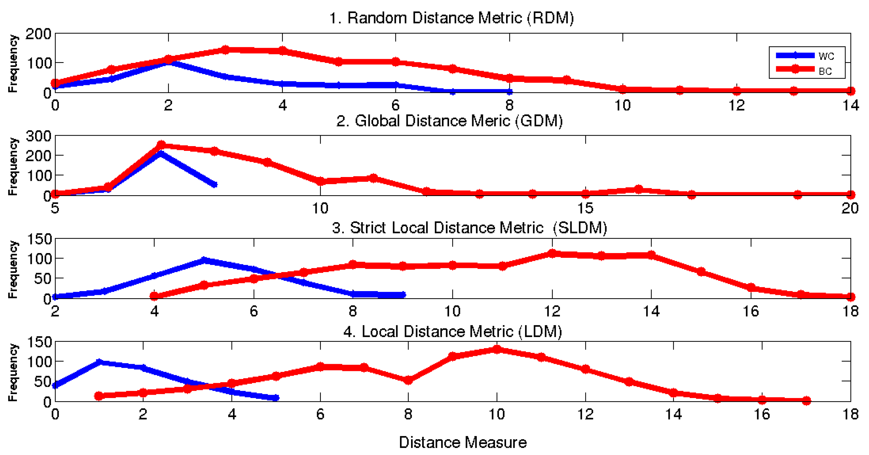
Figure 2 illustrates the different distance metric computational spaces. Let us assume a system is designed for
U different classes, where for any class
u there are
R prototypes (templates)
. Also, a class
v provides a set of
J questioned samples
. The distance between a questioned sample
and a prototype
is
. The distances between all the questioned and prototypes samples constitute a dissimilarity matrix, where each row contains distances from a specific query to all of the prototypes.
Where questioned and prototype samples belong to the same class, i.e.,
, the distance sample is a WC sample (black cells in
Figure 2). On the other hand, if questioned and prototype samples belong to different classes, i.e.,
, then the distance sample is a BC sample (white cells in
Figure 2). An ideal distance metric implies that all the WC distances have zero values, while all the BC distances have large values. This occurs when the employed metric
d absorbs all the WC variabilities, and detects all the BC similarities. The proposed approach aims to enlarge the separation between the BC and WC distance ranges, such that a simple distance threshold rule (like that involved in error correcting codes) produces accurate classification.
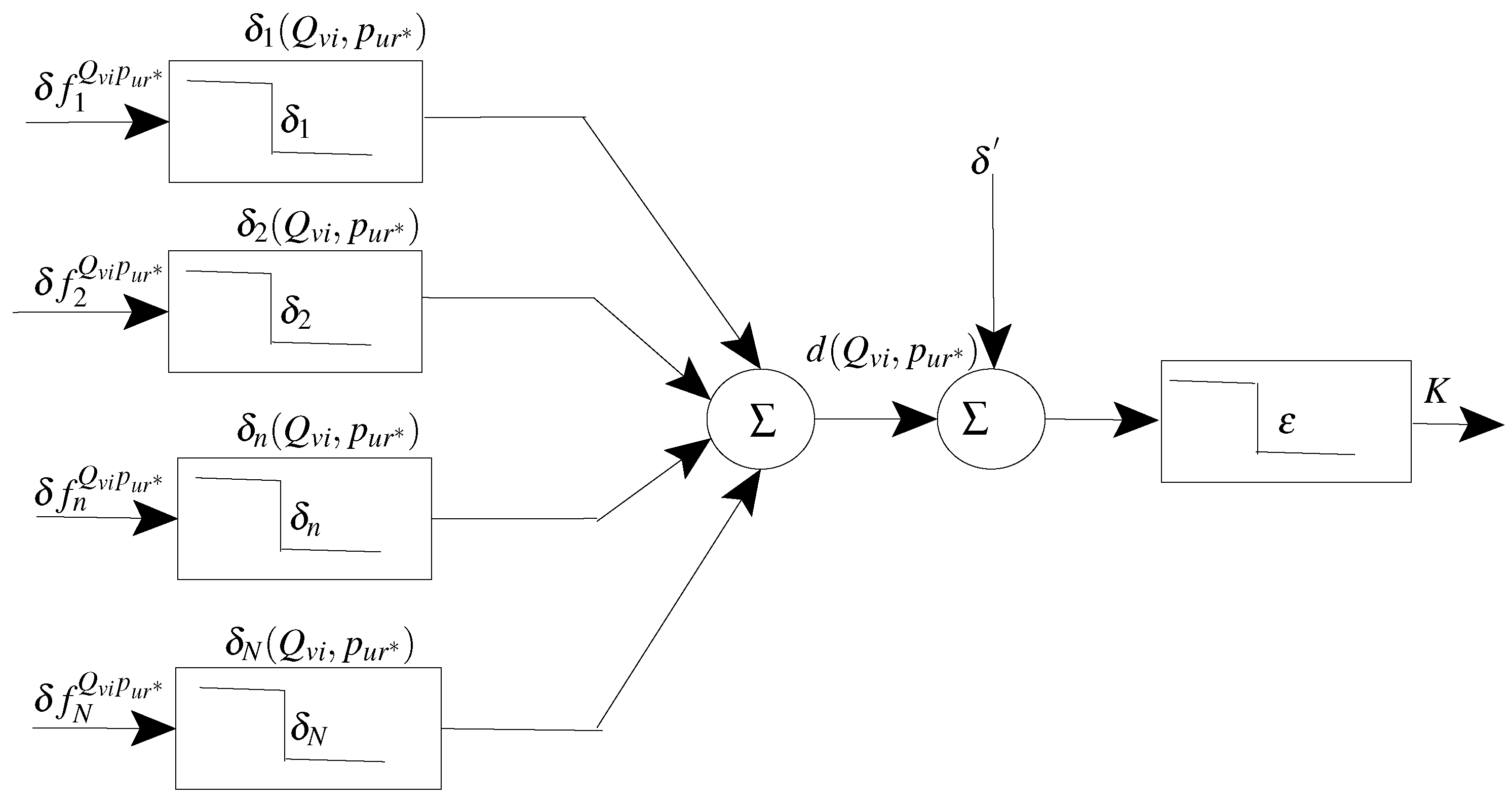
As shown in the figure, a distance measure accumulates some distance elements that are computed in the FD space, where the distance between a query
and a prototype
is measured by the distance between their feature representations
and
, respectively (see Equations (
1)–(
4)). To enlarge the separation between the WC and BC ranges, individual distance elements
should be designed properly such that the WC instances will have low values and the BC instances high values. Since a distance element relies on a specific feature
and its associated tolerance
, these building blocks should be optimized accordingly.
In the case of signature-based bio-cryptography systems, the optimization of the aforementioned distance metric is a challenging task since a concise representation must be selected from high-dimensional representations, especially when only a few positive samples and almost no forgery samples are available for training. We tackle this challenging problem by proposing a hybrid Global-Local learning framework that also achieves a trade-off between global and local distance metric approaches [
23]. The global learning process overrides the curse -of -dimensionality by using huge numbers of samples of a development dataset for learning in the original high-dimensional feature space. Therefore, it becomes feasible for the local learning process to learn in the resulting reduced space even when limited samples are available for training.
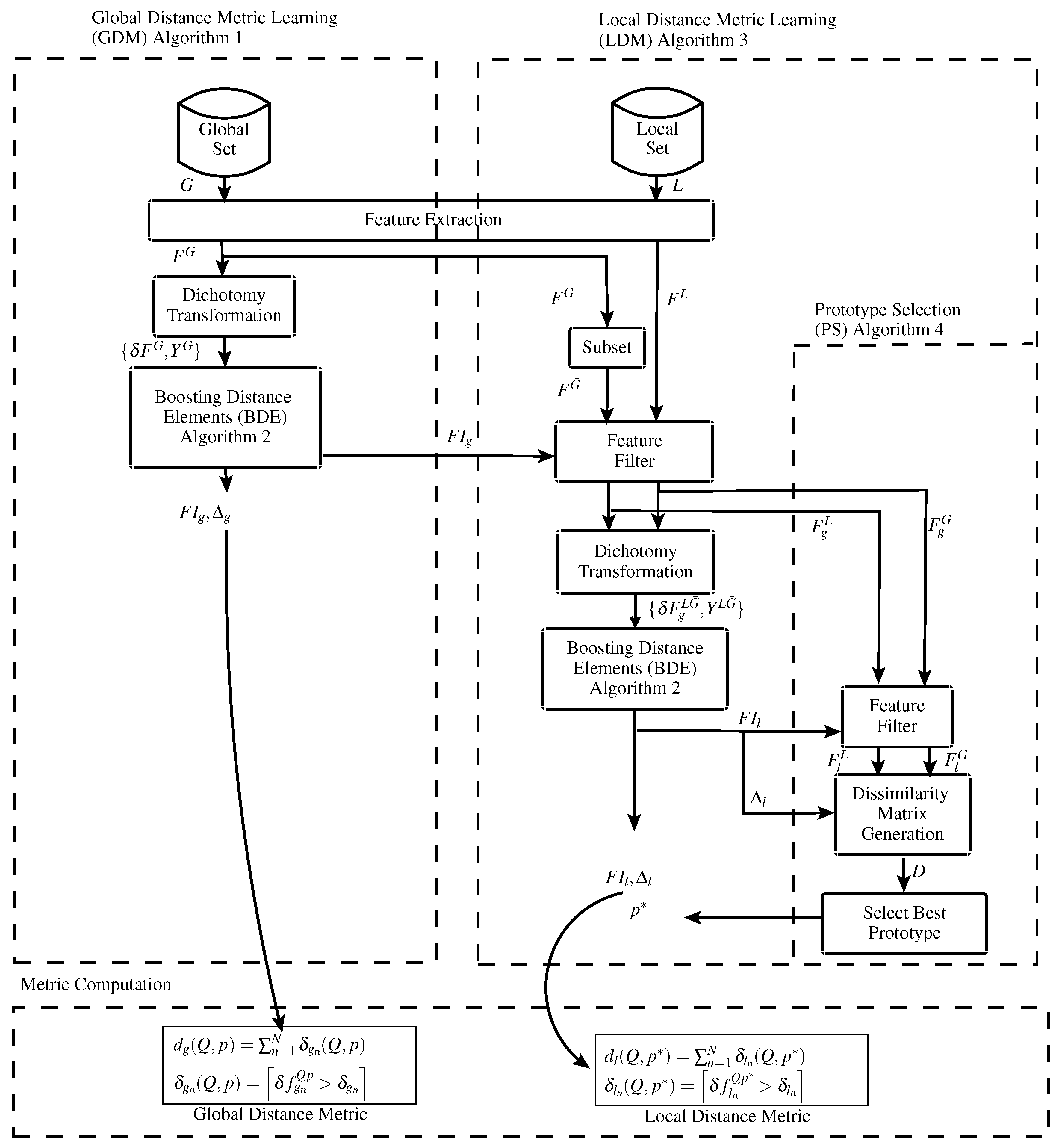
This section provides a detailed description of the proposed GLDM distance metric learning framework illustrated in
Figure 3 (please note that all the algorithms proposed in this paper are listed in the Figure). In the first step, a large number of samples of a global dataset is used to design a global distance metric that differentiates between WC and BC samples of the population. a preliminary feature space of huge dimensionality
M is produced and is reduced to a global space of dimensionality
through the application of a Boosting Distance Elements (BDE) process. This BDE process runs in the Feature-Dissimilarity (FD) space resulting from the application of a dichotomy transformation, where
distance elements are designed by selecting their constituting features and adjusting their tolerance values.
Then, once enrolling samples are available for a user, they are used to tune the global metric and produce a local (user-specific) distance metric. The local metric discriminates between the specific-class WC distances and the BC distances that are computed by comparing class samples to samples of other classes or forgeries. To this end, the local samples and some samples from the global dataset are represented in the global space of dimensionality
. Additional dichotomy transformation and BDE processes run in the reduced space to produce a local space of dimensionality
. Moreover, since different columns in the dissimilarity matrix might differ in accuracy (see
Figure 2), we determine the best signature prototype by selecting the most stable and discriminant column.
Finally, depending on whether or not a local solution is available, either a global or a local distance metric is computed by employing Equations (
1)–(
4), using the distance element constituents produced by the above steps. It is important to note that for both global and local distance metric computations, only the best
elements have been used since the metric produced is mainly designed for building FV systems that require a concise number of locking/unlocking elements.
4.3. Local Distance Metric Learning (LDM)
This process runs for every individual class (user), for tuning the global metric to the specific user. Algorithm 3 describes the LDM process. The local set (containing R samples) and a subset of the global set (containing I samples) are represented in the global representation of dimensionality produced by above global learning process. Then, they are translated to a global FD space producing distance samples , which consist of WC and BC samples of same dimensionality . These samples are sent to another BDE process that runs in the resulting FD space (as described in Algorithm 2), and it produces a local space of dimensionality consisting of a set of local feature indexes and their associated tolerance values . The resulting local representation could be employed directly to compute a local distance metric using any available prototype as a reference; however, we propose a prototype selection process which instead picks the most stable and discriminant prototype for enhancing the accuracy of the metric.
Algorithm 4 illustrates the prototype selection process. Firstly, the global representations
and
of the local and global sets, respectively, are translated to the reduced local space by means of the local feature indexes
(extracted in Step 6 of Algorithm 3). The produced local representations
and
are used to generate a dissimilarity matrix
D. To that end, the local tolerance values
(extracted in Step 6 of Algorithm 3) are used for the distance metric computations defined by Equations (
1)–(
4). The produced matrix
D is then used to select the most stable and discriminant prototype
.
| Algorithm 3 Local Distance Metric Learning (LDM) |
Input: Local set consists of R prototypes of local class, feature representation of global set G of dimensionality M (extracted in Algorithm 1), global feature indexes of dimensionality (output of Algorithm 1).
- 1:
Extract feature representation of high dimensionality M, where . - 2:
Select I samples from as a forgery subset . - 3:
Filter and with and produce global representations and of dimensionality , for global and local sets, respectively. - 4:
Produce dichotomy transformation , where , is a WC samples if i belongs to the local class, otherwise it is a BC sample. - 5:
Label dichotomy samples , so that for WC samples and for BC samples. - 6:
Run Boosting Distance Elements (BDE) process (Algorithm 2) using , as training set T local feature representation and associated tolerance , where . - 7:
Using the local feature indexes and local feature tolerance (both learned through above BDE step), select best prototype by running Algorithm 4.
Output: Local feature indexes and local feature tolerance both of dimensionality , best prototype . |
| Algorithm 4 Prototype Selection (PS) |
Input: Global feature representations and of dimensionality for global and local sets, respectively, local feature indexes , local feature tolerance .
- 1:
Filter and with and produce local representations and of dimensionality for global and local sets, respectively. - 2:
Generate dissimilarity matrix: , where is computed according to Equations ( 1)–( 4) using and . - 3:
Choose so that , where .
Output: Best prototype |
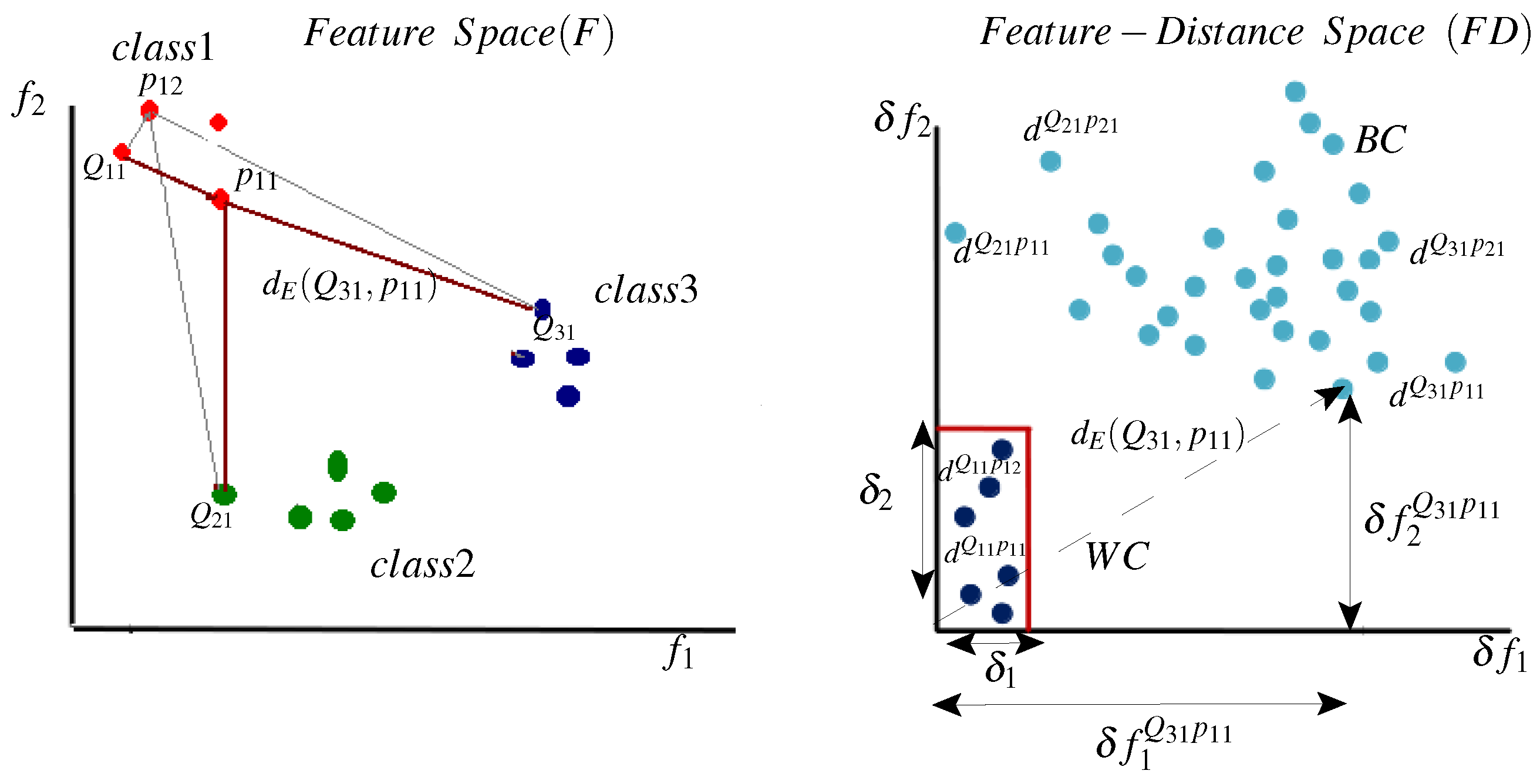
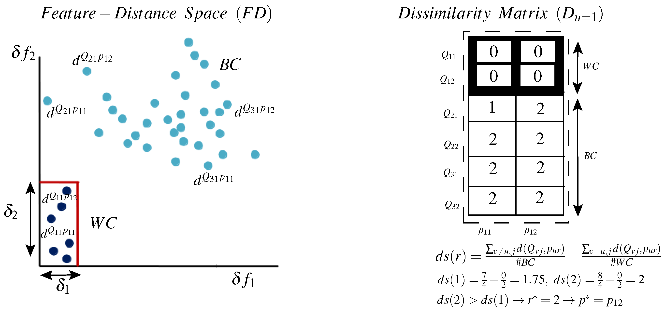
Figure 5 illustrates the prototype selection method by analyzing a dissimilarity matrix
D and its relation to the
representation space. On the left side, the WC and BC samples are represented in the
space. It is obvious that different prototypes (different columns in the matrix
D) produce different distance values, where significant variability exists for the WC and the BC classes. Moreover, in this space, it is not clear which prototype is the most informative. On the right side, distance samples
are projected to a dissimilarity matrix
, where each row contains distances between a specific query to all prototypes and each column contains distances between all queries to a specific prototype. Here, we investigate a part of
D (see
Figure 4) for a specific class
. Further, for simplicity, only two prototypes are shown for class 1 (
and
), and few query samples have been used (two queries for the local class
and
and two queries for each of the global classes 2 and 3). However, practical matrices could have a high number of prototypes (columns) and a high number of queries (rows). Moreover, this illustrative matrix is generated based on two features only (
and
), i.e.,
, and so the distance values
. Nevertheless, practical problems might include higher dimensionality. For instance, for
the distance values
.
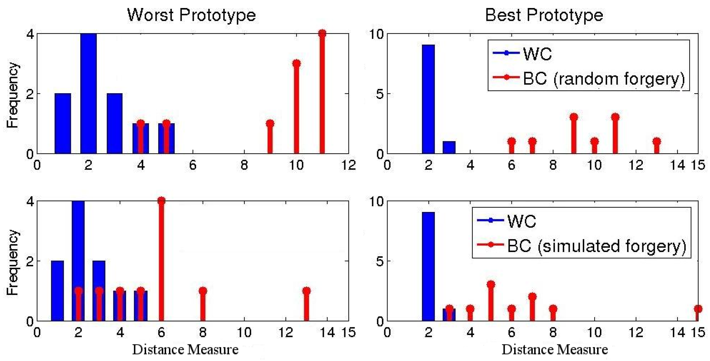
It is clear that the dissimilarity matrix provides an easier way of ranking prototypes according to their discriminative power. For instance, for class 1, is more discriminative than because for all BC samples, whereas for , (because ). Thus, for this class, measuring the distance relative to results in more isolated WC and BC distance ranges.
To automate the dissimilarity matrix analysis and the selection of the best prototype, we propose a distance separability measure:
The left part of the above equation measures the discriminative power of a prototype where high values indicate a large separation between global and local samples (BC distances). The right side for its part measures the stability of a prototype in which low values indicate a small separation between local samples (WC distances). Accordingly, we select the prototype that maximizes this distance separability measure and the best prototype is given by:
Finally, after the best prototype is selected, the optimal local distance metric
is computed in accordance with Equations (
1)–(
4) with reference to
.
