Abstract
The brain storm optimization (BSO) algorithm has received increased attention in the field of evolutionary computation. While BSO has been applied in numerous industrial scenarios due to its effectiveness and accessibility, there are few theoretical analysis results about its running time. Running-time analysis can be conducted through the estimation of the upper bounds of the expected first hitting time to evaluate the efficiency of BSO. This study estimates the upper bounds of the expected first hitting time on six single individual BSO variants (BSOs with one individual) based on the average gain model. The theoretical analysis indicates the following results. (1) The time complexity of the six BSO variants is in equal coefficient linear functions regardless of the presence or absence of the disrupting operator, where n is the number of the dimensions. Moreover, the coefficient of the upper bounds on the expected first hitting time shows that the single individual BSOs with the disrupting operator require fewer iterations to obtain the target solution than the single individual BSOs without the disrupting operator. (2) The upper bounds on the expected first hitting time of single individual BSOs with the standard normally distributed mutation operator are lower than those of BSOs with the uniformly distributed mutation operator. (3) The upper bounds on the expected first hitting time of single individual BSOs with the mutation operator are approximately twice those of BSOs with the mutation operator. The corresponding numerical results are also consistent with the theoretical analysis results.
1. Introduction
The swarm intelligence algorithm is one of the nature-inspired optimization algorithms that simulates the behavior of biological groups in nature [1,2,3]. Over the past two decades, many different types of swarm intelligence algorithms have been proposed, such as particle swarm optimization (PSO) [4,5], ant colony optimization (ACO) [6,7], artificial bee colony (ABC) [8,9], and brain storm optimization (BSO) [10,11,12]. Different from traditional methods, these algorithms solve problems by simulating the behavior of animal or human groups, with higher flexibility and adaptability.
BSO, a novel swarm intelligence algorithm, is inspired by the human brainstorming process. It is a continuous evolutionary algorithm that simulates the collective behavior of human beings. In recent years, BSOs have seen various practical applications in power systems [13,14,15,16], aviation design [17,18,19], mobile robot path planning [20,21], antenna design [22], financial optimization [23,24,25], and many other fields [26,27,28,29,30].
In addition, the theoretical analysis of BSO is also very important, especially for the practical application of BSO. The theoretical analysis benefits researchers in enabling them to understand the mechanism of the algorithm in guiding its design, improvement, and application in practice. The theoretical analysis can be divided into convergence analysis and running-time analysis. Zhou et al. [31], Qiao et al. [32], and Zhang et al. [33] have performed corresponding convergence analyses on BSO. The BSO–CAPSO algorithm, proposed by Alkmini [1], effectively enhances the computational efficiency of BSO through hybridization with chaotic accelerated particle swarm optimization. However, there are few works on the running-time analysis of BSO.
Some theoretical methods have been proposed as general analysis tools to investigate the running time of random heuristic algorithms, including the fitness level method [34], drift analysis method [35], switch analysis method [36], wave model [37], etc. These methods are mainly used to analyze discrete random heuristic algorithms. In contrast, fewer theoretical analysis results have been obtained for continuous random heuristic algorithms [38,39,40]. However, a large number of practical application problems are continuous. Therefore, the running time of continuous random heuristic algorithms has important research significance. To analyze the running time of continuous random heuristic algorithms, Huang et al. [41] proposed the average gain model.
Huang et al. [41,42] and Zhang et al. [43] used an average gain model to evaluate the expected first hit time of the ()-evolutionary algorithm (() EA), evolutionary strategy (ES), and covariance matrix adaptation evolution strategy (CMA-ES). The concept of the first hit time refers to the minimum number of iterations required before the algorithm finds an optimal solution [35]. The expected first hit time represents the average number of iterations needed to find the optimal solution, which actually reflects the average time complexity of the algorithm [44]. Wang [45] employed the average gain model to analyze the computational efficiency of the proposed swarm intelligence algorithm and provided theoretical evidence for its effectiveness. Therefore, the expected first hit time is a core metric in runtime analysis. Based on the average gain model, the expected first hit time of BSO is deeply analyzed in this paper.
The core of BSO consists of three key components: clustering, interruption, and update. The mutation operator plays an important role in BSO and is included in the interrupt operation and update operation. Specifically, the mutation operator helps the algorithm to jump out of the local optimal solution and further explore a broader search space by introducing random factors in the search process. For example, Zhan et al. [46] proposed an improved BSO (MBSO) in which the mutation operator employs a novel thought difference strategy (IDS). This strategy takes advantage of the thought differences among individuals in the group and increases the diversity of the group by introducing random factors, thus increasing the probability of the algorithm finding the global optimal solution. In addition, El-Abd [47] improved the step equation of the mutation operator and improved the performance of BSO by adjusting the step size and distribution. This improvement helps the algorithm to balance the local search and the global search better, so that the algorithm can find the global optimal solution more effectively when solving complex optimization problems.
The time complexity of the single individual BSO is analyzed in this paper based on the research process from simple to complex. The single individual BSO without the disrupting operation is the same as the (1+1) ES [41]. However, the corresponding results can explain the influence of the mutation operator and disrupting operator on the time complexity of BSO. In this paper, we choose the three most classic and representative distributions, , , and , as the analysis objects for the mutation operator. Therefore, six BSO variants are obtained as the analyzed algorithms based on the combination of three mutation operators and the presence or absence of a disrupting operator.
The remainder of this paper is organized as follows. Section 2 introduces the process of BSO and the mathematical model of running-time analysis for BSO. Section 3 provides the theoretical analysis results for the running-time analysis of three different BSO variants. Section 4 presents the corresponding experimental results to evaluate the theoretical results. Finally, Section 5 concludes the paper.
2. Mathematical Model for Running-Time Analysis of BSO
2.1. Brain Storm Optimization
BSO was proposed by Shi [48,49] in 2011, and it is simple in concept and easy to implement. BSO can be simplified as follows.
In Steps 4 and 5, the new solution is generated by , where x is the original individual, is the newly generated individual, and is a vector generated according to the mutation operator. In this paper, we focus on the running time of BSO with three different mutation operators. The same mutation operators are used to generate new individuals in both Steps 4 and 5. The superposition of different mutation operators is not considered in this work.
To accurately observe the effects of the disrupting and updating operations on the running time of BSO, we select a single individual form of BSO as the analyzed object. The single individual BSO framework simplifies the effect of the population size, which helps to evaluate the effect of the disrupting and updating operations on the running time. Furthermore, following the principle from simple to difficult, the single individual BSO is a suitable starting point for the running-time analysis of BSO. Moreover, the randomness of and the design of the operations in Steps 4 and 5 are derived from the mutation operator design of evolutionary programming [50,51]. Therefore, the conclusion of this analysis will have positive implications for the study of similar mutation operators in evolutionary programming algorithms.
2.2. Stochastic Process Model of BSO
BSO can be represented as a stochastic process. In this section, we introduce the terminology for the analysis of the running time of BSO.
Definition 1
(Hill-climbing task). Given a search space and a fitness function , the hill-climbing task is to find a solution where the fitness of reaches the target value H, where .
In this paper, we focus on analyzing the BSO running time in the hill-climbing task of a continuous search space.
Definition 2
(State of BSO). The state of BSO at the t-th iteration is defined as , where λ is the size of the population, and .
Definition 3
(State space of BSO). The set of all possible BSO states is called the state space of BSO, denoted as
An optimization problem is a mapping from a decision space to an objective space, and the state space of BSO represents the corresponding decision space.
Definition 4
(Expected first hitting time). Let be a stochastic process, where, for any , holds. Suppose that is the Euclidean distance value of the t-th iteration state of BSO to the target solution, and the target threshold , the first hitting time [35] of the ε-approximation solution, can be defined by
Therefore, the expected first hitting time [44] of BSO can be denoted with .
The expected first hit time refers to the average number of iterations required for the BSO algorithm to reach the target fitness value. This metric can more accurately measure the performance of an algorithm because it takes into account the probability distribution of the algorithm over different iterations. Through this metric, we can evaluate the average time complexity of the algorithm in finding the optimal solution, so as to better understand the efficiency of the algorithm.
2.3. Running-Time Analysis of BSO Based on Average Gain Model
Inspired by drift analysis [52] and the idea of Riemann integrals [53], Huang et al. [41] proposed the average gain model. Zhang et al. [43] separated this model by introducing the concepts of the supermartingale and stopping time. Based on the former research results [41,43] of the average gain model, Huang et al. [42] proposed an experimental method to estimate the running time of the continuous evolution algorithms.
The expected one-step variation
is called the average gain, where is a stochastic process, and . The -algebra contains all the events generated by . All the information observed from the original population to the t-th iteration is recorded in .
Based on Definition 2, is the state of BSO at the t-th iteration. The process of BSO in solving the hill-climbing task is considered as the gradual process of the stochastic state from the initial population to the population that contains the optimal solution. Let be the highest fitness value of individuals in . is used to measure the distance of the current population to the population of the target value. , where is the fitness value of the optimal solution. Obviously, is a non-negative stochastic process.
The state of BSO in the -th iteration only depends on . In other words, the stochastic process can be modeled by a Markov chain [42]. Similarly, can also be regarded as a Markov chain. In this case, the average gain can be simplified to . Based on Th. 2 of [43], the expectation of of BSO can be estimated as follows.
Theorem 1.
Suppose that is a stochastic process associated with BSO, where for all . Let be a monotonically increasing and integrable function. If and , it holds for that
Theorem 1 shows the upper bounds on the expected first hitting time of BSO based on the average gain model. The average gain plays a key role in analyzing the first hitting time of the -approximation solution for BSO. The higher average gain indicates a more efficient iteration of the optimization process.
3. Running-Time Analysis of BSO Instances for Equal Coefficient Linear Functions
In this section, we present the theoretical analysis results based on the average gain model to analyze the expected first hitting time of BSO for equal coefficient linear functions. The running time of BSO with three different mutation operators is analyzed from the perspective of whether the disrupting operation exists. In this paper, we refer to the BSO without a disrupting operation as BSO-I, and the BSO with a disrupting operation as BSO-II.
On this basis, the equal coefficient linear functions are selected as the research object [54,55,56]. These functions are a form of basic continuous optimization problem whose function expression is as follows:
where . It is assumed that the function starts from the origin and sets the target fitness value to , where . The objective of optimizing the equal coefficient linear function is to find a solution , such that .
The mutation operator that obeys the Gaussian distribution and the uniform distribution is selected for the evaluation of BSO. The Gaussian distribution and uniform distribution are common tools for the design of mutation operators [50,51,57], so it is representative to select these two distributions as research cases.
3.1. Case Study of BSO without Disrupting Operator
Since the single individual BSO is analyzed in this paper, is equal to 1 in the state of BSO. The BSO of a single individual has only one individual, so represents both the optimized individual and the random state of the algorithm. The procedure of single individual BSO can be described as follows when the disrupting operation does not exist (i.e., Step 4 in Algorithm 1 is ignored).
| Algorithm 1 Brain Storm Optimization (BSO) |
|
is the t-th generation of the algorithm.
is defined as the Euclidean distance of the t-th iteration to the optimal solution. The gain at t-th is given by
3.1.1. When
If the mutation operator obeys the standard normal distribution , the distribution function of is as presented by Lemma 1.
Lemma 1.
For BSO-I, if its mutation operator obeys , the distribution function of the gain is
Proof.
Since , are independent of each other. All of the satisfy the additivity of the normal distribution, so obeys the distribution of .
According to Step 4 and Step 5 of Algorithm 2, the ()-th individual is
| Algorithm 2 BSO-I |
|
According to the definition of , where ,
- (1)
- If ,
- (2)
- If ,
Hence, the distribution function of is shown as .
- (1)
- If , according to the definition of where , it has .
- (2)
- If , the probability density function of is symmetric in the y axis, so .
- (3)
- If , .
Lemma 1 holds. □
Theorem 2 is presented based on the above proof.
Theorem 2.
If the mutation operator of BSO-I obeys , the upper bound on the expected first hitting time to reach the target fitness value is derived as follows.
Proof.
It is assumed that the algorithm starts from the origin at initialization, where , i.e.,
According to Theorem 1, the upper bound on the expected first hitting time is derived as
Theorem 2 holds. □
Theorem 2 indicates that for BSO-I, if its mutation operator obeys , the computational time complexity of BSO-I for the equal coefficient linear function is .
3.1.2. When
The uniform distribution function does not satisfy additivity like the normal distribution function. The Lindeberg–Levy center limit theorem [58] can provide an idea to find the distribution of . The Lindeberg–Levy center limit theorem is introduced below.
Suppose that is a sequence of independent and identically distributed random variables with and ; let
then
is satisfied for any real number y.
The Lindeberg–Levy center limit theorem [58] shows that if n is sufficiently large, , it has . Generally, the case of higher dimensions requires more attention in the study of the computational time complexity of algorithms. If the mutation operator obeys , the distribution function of can be represented by Lemma 2.
Lemma 2.
For BSO-I, if its mutation operator obeys , the distribution function of the gain is
Proof.
According to the definition of , where .
- (1)
- If .
- (2)
- If , where , and are independent of each other. According to the Lindeberg–Levy center limit theorem, obeys .
Hence, the distribution function of is .
- (1)
- If , .
- (2)
- If , .
- (3)
- If , .
Lemma 2 holds. □
Theorem 3 is presented based on the above proof.
Theorem 3.
For BSO-I, if its mutation operator obeys , the upper bound on the expected first hitting time to reach the target fitness value is derived as follows.
The proof of this theorem is based on the same principle as Theorem 2. The detailed derivation is given as follows.
Proof.
According to Lemma 2, we have
and the algorithm starts from the origin at initialization, , i.e., . According to Theorem 1, the upper bound on the expected first hitting time is derived as
Theorem 3 indicates that if the mutation operator of BSO-I obeys , its computational time complexity is for the equal coefficient linear function.
3.1.3. When
If the mutation operator obeys , the distribution function of can be represented by Lemma 3.
Lemma 3.
For BSO-I, if its mutation operator obeys , the distribution function of the gain is
The proof of this lemma is based on the same principle as Lemma 2.
Proof.
According to the definition of ,
- (1)
- If .
- (2)
- If .
Since , are independent of each other, according to the Lindeberg–Levy center limit theorem, obeys .
Hence, the distribution function is
- (1)
- If , .
- (2)
- If , .
- (3)
- If , .
□
According to Lemma 3 and Theorem 1, Theorem 4 can be inferred.
Theorem 4.
For BSO-I, if its mutation operator obeys , the upper bound on the expected first hitting time to reach the target fitness value is derived as
The proof of this theorem is based on the same principle as Theorem 2. The proof is given as follows.
Proof.
According to Lemma 3, we have
and the algorithm starts from the origin at initialization, , i.e., . According to Theorem 1, the upper bound on the expected first hitting time is derived as
Theorem 4 indicates that if the mutation operator of BSO-I obeys , its computational time complexity for the equal coefficient linear function is .
The time complexity of BSO-I with three different mutation operators is . In the next section, we will discuss the running time of BSO considering the case with a disrupting operation.
3.2. Case Study of BSO with Disrupting Operator
Based on the average gain model, this section analyzes the upper bounds of the expected first hit time in three BSO cases. When interference operations are added to the single individual BSO, the algorithm process can be simplified as follows.
In Algorithm 3, the disrupting operations, which are executed with a small probability, are shown in Steps 3 to 6. Let indicate that replacement occurs, while indicates that no replacement occurs.
| Algorithm 3 BSO-II |
|
To highlight the effect of each mutation operator on the algorithm, we choose the same mutation operators of BSO-I in Steps 5 and 8 to generate new individuals. As a result, , where mutation operator parameter and follow the same distribution.
Here, is still the t-th individual of the algorithm. We have , and the corresponding gain at t is given by .
3.2.1. When
- (1)
- If , it is the same as the result of the case with no disrupting operation in Section 3.1, and the average gain is
- (2)
- If and the mutation operator obeys , the distribution function of is represented by Lemma 4.
Lemma 4.
For BSO-II, if its mutation operator obeys and , the distribution function of the gain is .
Proof.
According to Step 12 and Step 13 of Algorithm 3, the ()-th individual is .
According to the definition of ,
- (1)
- If .
- (2)
- If ,
Since , , and are independent of each other, are also independent of each other. All of and satisfy the additivity of the normal distribution. As a result, obeys .
Hence, the distribution function of is .
- (1)
- If , .
- (2)
- If , .
- (3)
- If , .
Lemma 4 holds. □
Based on the above proofs, we can conclude that
Assume that the probability is equal to 0.2 [59]; Theorem 5 can be obtained according to Theorem 1.
Theorem 5.
For BSO-II, if its mutation operator obeys , the upper bound on the expected first hitting time to reach the target fitness value is derived as follows.
Proof.
The algorithm starts from the origin at initialization, , i.e., . According to Theorem 1, the upper bound on the expected first hitting time is derived as
Theorem 5 holds. □
According to the proof of Theorem 5, if the mutation operator of BSO-II obeys , its computational time complexity for the equal coefficient linear function is .
3.2.2. When
- (1)
- If , the result is the same as the case in Section 3.1 with no disrupting operation. The average gain is
- (2)
- If and the mutation operator obeys , the distribution function of is represented by Lemma 5.
Lemma 5.
If the mutation operator of BSO-II obeys and , the distribution function of the gain is .
The proof of this lemma is based on the same principle as Lemma 4. The detailed derivation is given as follows.
Proof.
According to the definition of ,
- (1)
- If .
- (2)
- If
Since , , and are independent of each other, are also independent of each other. obeys according to the Lindeberg–Levy center limit theorem.
Hence, the distribution function is
- (1)
- If , .
- (2)
- If , .
- (3)
- If , .
□
Theorem 6 can be concluded based on Lemma 5 and Theorem 1.
Theorem 6.
If the mutation operator of BSO-II obeys , the upper bound on the expected first hitting time to reach the target fitness value is derived as follows.
The proof of this theorem is based on the same principle as Theorem 5. The detailed derivation is presented as follows.
Proof.
According to Lemma 5, we have
Suppose that the probability ; according to Theorem 1, the following conclusions can be drawn:
The algorithm starts from the origin at initialization, , i.e., . According to Theorem 1, the upper bound on the expected first hitting time is derived as
Theorem 6 indicates that for BSO-II, if its mutation operator obeys , the computational time complexity of BSO-II for the equal coefficient linear function is .
3.2.3. When
- (1)
- If , the result is the same as the case in Section 3.1 with no disrupting operation. The average gain is
- (2)
- If , and the mutation operator obeys , the distribution function of is represented by Lemma 6.
Lemma 6.
If the mutation operator of BSO-II obeys and , its distribution function of the gain is
The proof of Lemma 6 is based on the same principle as Lemma 4. The proof is given as follows, which is used to support the proof of Theorem 7.
Proof.
According to the definition of ,
- (1)
- If .
- (2)
- If
Since , , and are independent of each other, are also independent of each other. obeys according to the Lindeberg–Levy center limit theorem.
Hence, the distribution function is
- (1)
- If , .
- (2)
- If , .
- (3)
- If , .
□
Theorem 7.
If the mutation operator of BSO-II obeys , the upper bound on the expected first hitting time to reach the target fitness value is derived as
The proof of this theorem is based on the same principle as Theorem 5. The proof is given as follows.
Proof.
According to Lemma 6, we have
Suppose that the probability ; according to Theorem 1, the following conclusions can be drawn:
The algorithm starts from the origin at initialization, , i.e., . According to Theorem 1, the upper bound on the expected first hitting time is derived as
Theorem 7 indicates that if the mutation operator of BSO-II obeys , its computational time complexity for the equal coefficient linear function is .
3.3. Summary
Overall, we summarize the theoretical analysis results of the running-time analysis of the single individual BSO in solving the n-dimensional equal coefficient linear function in six different situations. The theoretical analysis results are shown in Table 1. The time complexity of the single individual BSO in these six cases is . However, the coefficients in the display expressions are different.

Table 1.
Analysis of the running time of BSO in six different situations.
Table 1 shows the correlation between the expected first hitting time, the dimension n, the slope k, and the parameter a. The upper bounds on the expected first hitting time of BSO-II are lower than those of BSO-I. This means that the performance of BSO-II is better than that of BSO-I in solving the equal coefficient linear function. The disrupting operation in BSO helps to reduce the running time of the algorithm. Moreover, the upper bounds on the expected first hitting time of the algorithm using the standard normal distribution mutation operator are lower than those of the algorithms with the uniform distribution mutation operator. In addition, the upper bounds on the expected first hitting time of the algorithm using the mutation operator are approximately two times higher than those of the algorithm using the mutation operator.
4. Experimental Results
In Section 3, we obtain the theoretical analysis results of the expected first hitting time of single individual BSOs through the average gain model. To verify the correctness of the analysis results, numerical experiments are presented in this section.
As the number of samples increases, the arithmetic mean will gradually approach true mathematical expectations based on the Wiener–Khinchine theorem of large numbers [58]. The Wiener–Khinchine theorem of large numbers is introduced as follows.
Suppose that is a sequence of independent and identically distributed random variables with ; for any , the following equation will hold.
The Wiener–Khinchine theorem of large numbers indicates that if the number of samples is sufficiently large, the mathematical expectations are approximately equal to the mean of samples . Therefore, we use the arithmetic mean of the first hitting time of multiple experiments to estimate the actual expected first hitting time.
In this section, the parameters of the proposed approach are set as follows. The fixing error is , the initial individual is , the slope is , and the target fitness parameter is . The problem dimension n is set from 10 to 280. BSO-I and BSO-II are conducted on the n-dimensional equal coefficient linear function for 300 runs for each dimension. The termination criterion for each experiment is that the error of the optimal solution should be below a predefined threshold . Table 2 shows the numerical results of the practical expected first hitting time and the theoretical time upper bound, where , and is the first hitting time of the -approximation solution at the i-th run.
Table 2.
Comparison of the estimation of the expected first hitting time and the theoretical upper bounds.
As shown in Table 2, the experimental results strongly fit the theoretical upper bounds, indicating that the error between the theoretical upper bounds and the actual value is within . The points larger than the theoretical upper bounds are highlighted in boldface. The arithmetic mean of multiple experiments is used to estimate the expected first hitting time. In the real case, only the arithmetic mean of 300 experiments is used to estimate the expected first hitting time, which allows a certain statistical error. According to the central limit theorem, the results obtained from 300 independent experiments follow a normal distribution. The null hypothesis means that the mean value of the expected first hitting time in 300 experiments is less than or equal to the corresponding theoretical upper bounds. The corresponding significance level is with the T testing. Moreover, as shown in Figure 1, the actual expected running time is followed with the estimated result based on our proof. All the detailed results are shown in Table 3.
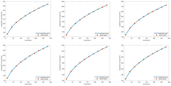
Figure 1.
The curve of the expected and the actual running time. The six figures, arranged from top to bottom and left to right, depict the three distributions corresponding to BSO-I and the three distributions corresponding to BSO-II, respectively.
Table 3.
Statistical results of hypothesis testing.
Table 3 provides the numerical results, where h represents the hypothetical result, p represents the p-value of the test, and is the confidence interval. As shown in the T testing of Table 3, and . The null hypothesis is accepted at the significance level . Therefore, the analytic expression of the running time of BSO obtained based on the average gain model can characterize the actual upper bounds of the running time of BSO in these six BSO variants.
5. Conclusions
The running time of six BSO variants for the equal coefficient linear function is analyzed in this paper based on the average gain model. The additivity of the normal distribution and the Lindeberg–Levy center limit theorem are applied to deal with the superposition of the normal distribution mutation operator and the uniform distribution mutation operator, respectively. Furthermore, the full expectation formula is utilized to deal with the problem of individual replacement with a certain probability in the disrupting operator. This paper also concludes the upper bounds on the expected first hitting time of the single individual BSO in equal coefficient linear functions.
The analysis results show that the time complexity of BSO-I and BSO-II is in the equal coefficient linear function. However, their coefficients are different. In the linear function with equal coefficients, the upper bound of the expected first hit time of BSO-II is smaller than that of BSO-I. In addition, the single individual BSO using the standard normally distributed mutation operator expects a lower upper bound on the first hit time than the corresponding algorithm using the uniformly distributed mutation operator. The upper bounds on the expected first hitting time of single individual BSOs with the mutation operator are approximately twice those of BSOs with the mutation operator.
In our future work, we will analyze the running time of the population-based BSO in the equal coefficient linear function. The running time of population-based BSOs in practical optimization problems is also an important topic. Moreover, it is crucial to extend our research to practical optimization problems that are encountered in real-world applications with complex constraints, non-linear relationships, or high-dimensional spaces.
Author Contributions
Conceptualization, G.M. and F.L.; methodology, G.M., F.L. and Y.H.; formal analysis, G.M. and Y.H.; investigation, D.L., J.S., X.Y. and H.H.; writing original draft preparation, F.L., D.L. and J.S.; writing review and editing, G.M. and Y.H. All authors have read and agreed to the published version of the manuscript.
Funding
This work is supported by the National Natural Science Foundation of China (62276103), Natural Science Foundation of Guangdong Province (2022A1515110058, 2022A1515011551), Guangdong Provincial Department of Education (No.2021KTSCX070, 2021KCXTD038, 2023KCXTD002), Guangzhou Science and Technology Planning Project (2023A04J1684), Doctor Starting Fund of Hanshan Normal University, China (No. QD20190628, QD2021201), Scientific Research Talents Fund of Hanshan Normal University, China (No. Z19113), The quality of teaching construction project of Hanshan Normal University (E22022, E23045), Research Platform Project of Hanshan Normal University (PNB221102), The quality of teaching construction project of Guangdong Provincial Department of Education in 2023 (No.350) and Guangdong Provincial Key Laboratory of Data Science and Intelligent Education (2022KSYS003).
Institutional Review Board Statement
Not applicable.
Data Availability Statement
Data are contained within the article.
Conflicts of Interest
The authors declare no conflict of interest.
References
- Michaloglou, A.; Tsitsas, N.L. A Brain Storm and Chaotic Accelerated Particle Swarm Optimization Hybridization. Algorithms 2023, 16, 208. [Google Scholar] [CrossRef]
- Slowik, A.; Kwasnicka, H. Nature inspired methods and their industry applications-swarm intelligence algorithms. IEEE Trans. Ind. Inform. 2017, 14, 1004–1015. [Google Scholar] [CrossRef]
- Xue, Y.; Jiang, J.; Zhao, B.; Ma, T. A self-adaptive artificial bee colony algorithm based on global best for global optimization. Soft Comput. 2018, 22, 2935–2952. [Google Scholar] [CrossRef]
- Liu, X.; Zhan, Z.; Gao, Y.; Zhang, J.; Kwong, S.; Zhang, J. Coevolutionary Particle Swarm Optimization With Bottleneck Objective Learning Strategy for Many-Objective Optimization. IEEE Trans. Evol. Comput. 2019, 23, 587–602. [Google Scholar] [CrossRef]
- Zhao, Q.; Li, C. Two-Stage Multi-Swarm Particle Swarm Optimizer for Unconstrained and Constrained Global Optimization. IEEE Access 2020, 8, 124905–124927. [Google Scholar] [CrossRef]
- Yu, X.; Chen, W.; Gu, T.; Yuan, H.; Zhang, H.; Zhang, J. ACO-A*: Ant Colony Optimization Plus A* for 3-D Traveling in Environments with Dense Obstacles. IEEE Trans. Evol. Comput. 2019, 23, 617–631. [Google Scholar] [CrossRef]
- Lyu, Z.; Wang, Z.; Duan, D.; Lin, L.; Li, J.; Yang, Y.; Chen, Y.; Li, Y. Tilting Path Optimization of Tilt Quad Rotor in Conversion Process Based on Ant Colony Optimization Algorithm. IEEE Access 2020, 8, 140777–140791. [Google Scholar] [CrossRef]
- Zhang, L.; Wang, S.; Zhang, K.; Zhang, X.; Sun, Z.; Zhang, H.; Chipecane, M.T.; Yao, J. Cooperative Artificial Bee Colony Algorithm with Multiple Populations for Interval Multiobjective Optimization Problems. IEEE Trans. Fuzzy Syst. 2019, 27, 1052–1065. [Google Scholar] [CrossRef]
- Kumar, D.; Mishra, K. Co-variance guided artificial bee colony. Appl. Soft Comput. 2018, 70, 86–107. [Google Scholar] [CrossRef]
- Cheng, S.; Qin, Q.; Chen, J.; Shi, Y. Brain storm optimization algorithm: A review. Artif. Intell. Rev. 2016, 46, 445–458. [Google Scholar] [CrossRef]
- Cheng, S.; Sun, Y.; Chen, J.; Qin, Q.; Chu, X.; Lei, X.; Shi, Y. A comprehensive survey of brain storm optimization algorithms. In Proceedings of the 2017 IEEE Congress on Evolutionary Computation (CEC), San Sebastián, Spain, 5–8 June 2017; pp. 1637–1644. [Google Scholar]
- Cheng, S.; Lei, X.; Hui, L.; Zhang, Y.; Shi, Y. Generalized pigeon-inspired optimization algorithms. Sci. China Inf. Sci. 2019, 62, 120–130. [Google Scholar] [CrossRef]
- Xiong, G.; Shi, D.; Zhang, J.; Zhang, Y. A binary coded brain storm optimization for fault section diagnosis of power systems. Electr. Power Syst. Res. 2018, 163, 441–451. [Google Scholar] [CrossRef]
- Wang, Z.; He, J.; Xu, Y.; Crossley, P.; Zhang, D. Multi-objective optimisation method of power grid partitioning for wide-area backup protection. IET Gener. Transm. Distrib. 2018, 12, 696–703. [Google Scholar] [CrossRef]
- Ogawa, S.; Mori, H. A Hierarchical Scheme for Voltage and Reactive Power Control with Predator-Prey Brain Storm Optimization. In Proceedings of the 2019 20th International Conference on Intelligent System Application to Power Systems (ISAP), New Delhi, India, 10–14 December 2019; pp. 1–6. [Google Scholar] [CrossRef]
- Matsumoto, K.; Fukuyama, Y. Voltage and Reactive Power Control by Parallel Modified Brain Storm Optimization. In Proceedings of the 2020 International Conference on Artificial Intelligence in Information and Communication (ICAIIC), Fukuoka, Japan, 19–21 February 2020; pp. 553–558. [Google Scholar] [CrossRef]
- Soyinka, O.K.; Duan, H. Optimal Impulsive Thrust Trajectories for Satellite Formation via Improved Brainstorm Optimization. In Proceedings of the Advances in Swarm Intelligence; Tan, Y., Shi, Y., Niu, B., Eds.; Springer: Cham, Switzerland, 2016; pp. 491–499. [Google Scholar]
- Li, J.; Duan, H. Simplified brain storm optimization approach to control parameter optimization in F/A-18 automatic carrier landing system. Aerosp. Sci. Technol. 2015, 42, 187–195. [Google Scholar] [CrossRef]
- Zhang, C.; Xu, X.; Shi, Y.; Deng, Y.; Li, C.; Duan, H. Binocular Pose Estimation for UAV Autonomous Aerial Refueling via Brain Storm Optimization. In Proceedings of the 2019 IEEE Congress on Evolutionary Computation (CEC), Wellington, New Zealand, 10–13 June 2019; pp. 254–261. [Google Scholar] [CrossRef]
- Tuba, E.; Strumberger, I.; Zivkovic, D.; Bacanin, N.; Tuba, M. Mobile Robot Path Planning by Improved Brain Storm Optimization Algorithm. In Proceedings of the 2018 IEEE Congress on Evolutionary Computation (CEC), Rio de Janeiro, Brazil, 8–13 July 2018; pp. 1–8. [Google Scholar] [CrossRef]
- Li, G.; Zhang, D.; Shi, Y. An Unknown Environment Exploration Strategy for Swarm Robotics Based on Brain Storm Optimization Algorithm. In Proceedings of the 2019 IEEE Congress on Evolutionary Computation (CEC), Wellington, New Zealand, 10–13 June 2019; pp. 1044–1051. [Google Scholar] [CrossRef]
- Aldhafeeri, A.; Rahmat-Samii, Y. Brain Storm Optimization for Electromagnetic Applications: Continuous and Discrete. IEEE Trans. Antennas Propag. 2019, 67, 2710–2722. [Google Scholar] [CrossRef]
- Sun, Y. A Hybrid Approach by Integrating Brain Storm Optimization Algorithm with Grey Neural Network for Stock Index Forecasting. Abstr. Appl. Anal. 2014, 2014, 1–10. [Google Scholar] [CrossRef][Green Version]
- Xiong, G.; Shi, D. Hybrid biogeography-based optimization with brain storm optimization for non-convex dynamic economic dispatch with valve-point effects. Energy 2018, 157, 424–435. [Google Scholar] [CrossRef]
- Wu, Y.; Wang, X.; Xu, Y.; Fu, Y. Multi-objective Differential-Based Brain Storm Optimization for Environmental Economic Dispatch Problem. In Proceedings of the Brain Storm Optimization Algorithms: Concepts, Principles and Applications; Cheng, S., Shi, Y., Eds.; Springer: Cham, Switzerland, 2019; pp. 79–104. [Google Scholar]
- Ma, X.; Jin, Y.; Dong, Q. A generalized dynamic fuzzy neural network based on singular spectrum analysis optimized by brain storm optimization for short-term wind speed forecasting. Appl. Soft Comput. 2017, 54, 296–312. [Google Scholar] [CrossRef]
- Liang, J.J.; Wang, P.; Yue, C.T.; Yu, K.; Li, Z.H.; Qu, B. Multi-objective Brainstorm Optimization Algorithm for Sparse Optimization. In Proceedings of the 2018 IEEE Congress on Evolutionary Computation (CEC), Rio de Janeiro, Brazil, 8–13 July 2018; pp. 1–8. [Google Scholar] [CrossRef]
- Fu, Y.; Tian, G.; Fathollahi-Fard, A.M.; Ahmadi, A.; Zhang, C. Stochastic multi-objective modelling and optimization of an energy-conscious distributed permutation flow shop scheduling problem with the total tardiness constraint. J. Clean. Prod. 2019, 226, 515–525. [Google Scholar] [CrossRef]
- Pourpanah, F.; Shi, Y.; Lim, C.P.; Hao, Q.; Tan, C.J. Feature selection based on brain storm optimization for data classification. Appl. Soft Comput. 2019, 80, 761–775. [Google Scholar] [CrossRef]
- Peng, S.; Wang, H.; Yu, Q. Multi-Clusters Adaptive Brain Storm Optimization Algorithm for QoS-Aware Service Composition. IEEE Access 2020, 8, 48822–48835. [Google Scholar] [CrossRef]
- Zhou, Z.; Duan, H.; Shi, Y. Convergence analysis of brain storm optimization algorithm. In Proceedings of the 2016 IEEE Congress on Evolutionary Computation (CEC), Vancouver, BC, Canada, 24–29 July 2016; pp. 3747–3752. [Google Scholar] [CrossRef]
- Qiao, Y.; Huang, Y.; Gao, Y. The Global Convergence Analysis of Brain Storm Optimization. NeuroQuantology 2018, 16, 6. [Google Scholar] [CrossRef][Green Version]
- Zhang, Y.; Huang, H.; Hongyue, W.; Hao, Z. Theoretical analysis of the convergence property of a basic pigeon-inspired optimizer in a continuous search space. Sci. China Inf. Sci. 2019, 62, 86–94. [Google Scholar] [CrossRef]
- Sudholt, D. A New Method for Lower Bounds on the Running Time of Evolutionary Algorithms. IEEE Trans. Evol. Comput. 2013, 17, 418–435. [Google Scholar] [CrossRef]
- He, J.; Yao, X. Average Drift Analysis and Population Scalability. IEEE Trans. Evol. Comput. 2017, 21, 426–439. [Google Scholar] [CrossRef]
- Yu, Y.; Qian, C.; Zhou, Z.H. Switch Analysis for Running Time Analysis of Evolutionary Algorithms. IEEE Trans. Evol. Comput. 2015, 19, 777–792. [Google Scholar] [CrossRef]
- Li, Y.; Xiang, Z.; Ji, D. Wave models and dynamical analysis of evolutionary algorithms. Sci. China Inf. Sci. 2019, 62, 53–68. [Google Scholar]
- Lehre, P.K.; Witt, C. Concentrated Hitting Times of Randomized Search Heuristics with Variable Drift. In Proceedings of the Algorithms and Computation; Ahn, H.K., Shin, C.S., Eds.; Springer: Cham, Switzerland, 2014; pp. 686–697. [Google Scholar]
- Witt, C. Fitness levels with tail bounds for the analysis of randomized search heuristics. Inf. Process. Lett. 2014, 114, 38–41. [Google Scholar] [CrossRef]
- Yu, Y.; Qian, C. Running time analysis: Convergence-based analysis reduces to switch analysis. In Proceedings of the 2015 IEEE Congress on Evolutionary Computation (CEC), Sendai, Japan, 25–28 May 2015; pp. 2603–2610. [Google Scholar] [CrossRef]
- Huang, H.; Xu, W.; Zhang, Y.; Lin, Z.; Hao, Z. Runtime analysis for continuous (1 + 1) evolutionary algorithm based on average gain model. Sci. China Inf. Sci. 2014, 44, 811–824. [Google Scholar]
- Huang, H.; Su, J.; Zhang, Y.; Hao, Z. An Experimental Method to Estimate Running Time of Evolutionary Algorithms for Continuous Optimization. IEEE Trans. Evol. Comput. 2020, 24, 275–289. [Google Scholar] [CrossRef]
- Zhang, Y.; Huang, H.; Hao, Z.; Hu, G. First hitting time analysis of continuous evolutionary algorithms based on average gain. Clust. Comput. 2016, 19, 1323–1332. [Google Scholar]
- Yu, Y.; Zhou, Z.H. A new approach to estimating the expected first hitting time of evolutionary algorithms. Artif. Intell. 2006, 172, 1809–1832. [Google Scholar] [CrossRef]
- Wang, Y. Application of data mining based on swarm intelligence algorithm in financial support of livestock and poultry breeding insurance. Soft Comput. 2023. [Google Scholar] [CrossRef]
- Zhan, Z.; Zhang, J.; Shi, Y.; Liu, H. A modified brain storm optimization. In Proceedings of the 2012 IEEE Congress on Evolutionary Computation, Brisbane, QLD, Australia, 10–15 June 2012; pp. 1–8. [Google Scholar]
- El-Abd, M. Brain storm optimization algorithm with re-initialized ideas and adaptive step size. In Proceedings of the 2016 IEEE Congress on Evolutionary Computation (CEC), Vancouver, BC, Canada, 24–29 July 2016; pp. 2682–2686. [Google Scholar]
- Shi, Y. Brain Storm Optimization Algorithm. In Proceedings of the Advances in Swarm Intelligence; Tan, Y., Shi, Y., Chai, Y., Wang, G., Eds.; Springer: Berlin/Heidelberg, Germany, 2011; pp. 303–309. [Google Scholar]
- Shi, Y. An Optimization Algorithm Based on Brainstorming Process. Int. J. Swarm Intell. Res. 2011, 2, 35–62. [Google Scholar] [CrossRef]
- Yao, X.; Xu, Y. Recent advances in evolutionary computation. J. Comput. Sci. Technol. 2006, 21, 1–18. [Google Scholar] [CrossRef]
- Agapie, A.; Agapie, M.; Zbaganu, G. Evolutionary algorithms for continuous-space optimisation. Int. J. Syst. Sci. 2013, 44, 502–512. [Google Scholar] [CrossRef]
- He, J.; Yao, X. Drift analysis and average time complexity of evolutionary algorithms. Artif. Intell. 2001, 127, 57–85. [Google Scholar] [CrossRef]
- Hassler, U. Riemann Integrals. In Proceedings of the Stochastic Processes and Calculus: An Elementary Introduction with Applications; Springer: Cham, Switzerland, 2016; pp. 179–197. [Google Scholar]
- Jägersküpper, J. Combining Markov-chain analysis and drift analysis: The (1 + 1) evolutionary algorithm on linear functions reloaded. Algorithmica 2011, 59, 409–424. [Google Scholar] [CrossRef]
- Witt, C. Tight Bounds on the Optimization Time of a Randomized Search Heuristic on Linear Functions. Comb. Probab. Comput. 2013, 22, 294–318. [Google Scholar] [CrossRef]
- Hao, Z.; Huang, H.; Zhang, X.; Tu, K. A Time Complexity Analysis of ACO for Linear Functions. In Proceedings of the Simulated Evolution and Learning, 6th International Conference, SEAL 2006, Hefei, China, 15–18 October 2006. [Google Scholar]
- Jgersküpper, J. Algorithmic analysis of a basic evolutionary algorithm for continuous optimization. Theor. Comput. Sci. 2007, 379, 329–347. [Google Scholar] [CrossRef]
- Feller, W. An Introduction to Probability Theory and Its Applications; John Wiley & Sons: Hoboken, NJ, USA, 2008; Volume 2. [Google Scholar]
- Zhan, Z.H.; Chen, W.N.; Lin, Y.; Gong, Y.J.; Li, Y.L.; Zhang, J. Parameter investigation in brain storm optimization. In Proceedings of the 2013 IEEE Symposium on Swarm Intelligence (SIS), Singapore, 16–19 April 2013; pp. 103–110. [Google Scholar] [CrossRef]
Disclaimer/Publisher’s Note: The statements, opinions and data contained in all publications are solely those of the individual author(s) and contributor(s) and not of MDPI and/or the editor(s). MDPI and/or the editor(s) disclaim responsibility for any injury to people or property resulting from any ideas, methods, instructions or products referred to in the content. |
© 2024 by the authors. Licensee MDPI, Basel, Switzerland. This article is an open access article distributed under the terms and conditions of the Creative Commons Attribution (CC BY) license (https://creativecommons.org/licenses/by/4.0/).