A Hybrid RUL Prediction Framework for Lithium-Ion Batteries Based on EEMD and KAN-LSTM

Abstract

Accurately estimating the remaining useful life (RUL) of lithium-ion batteries in energy storage systems is critical for ensuring both the safety and reliability of the power grid. To address the complex nonlinear degradation behavior associated with battery aging, this study proposes a novel RUL prediction framework that integrates ensemble empirical mode decomposition (EEMD) with an ensemble learning algorithm. The approach first applies EEMD to decompose aging data into a residual component and several intrinsic mode functions (IMFs). The residual component is then modeled using a long short-term memory (LSTM) network, while the Kolmogorov–Arnold network (KAN) focuses on learning from the IMF components. These individual predictions are subsequently combined to reconstruct the overall capacity degradation trajectory. Experimental validation on real lithium-ion battery aging datasets demonstrates that the proposed method provides highly accurate RUL predictions, exhibits strong robustness, and effectively captures nonlinear characteristics under varying operating conditions. Specifically, the method achieves R² above 0.96 with absolute RUL errors within 2–3 cycles on NASA datasets, and maintains R² values above 0.91 with errors within 7–15 cycles on CALCE datasets. Furthermore, the optimal KAN hyperparameters for different IMF components are identified, offering valuable insights for multi-scale modeling and future model optimization.

1. Introduction

With the continuous expansion of modern power systems, increasing structural complexity and diversified load types pose significant challenges to system stability and reliability. Lithium-ion batteries (LIBs) are increasingly recognized as a viable alternative to traditional fossil fuels, making them increasingly prevalent in applications such as electric vehicles, aerospace, and electronic devices because of their high energy density, long cycle life, and environmentally friendly properties, offering great potential to alleviate energy consumption and environmental pressure [1,2,3,4,5,6,7,8,9]. However, during prolonged charge–discharge cycling, irreversible electrochemical reactions within LIBs cause degradation of electrode materials and gradual capacity fading [10,11,12,13]. Once the battery capacity falls below approximately 70% to 80% of its initial rated value, its performance and operational stability deteriorate significantly, and timely replacement becomes necessary. Continued operation in such a degraded state not only fails to meet system requirements but may also introduce serious safety risks with potentially catastrophic consequences [14,15,16,17,18,19]. The remaining useful life (RUL) of a lithium-ion battery represents the number of charge–discharge cycles achievable before its capacity falls below a specified threshold. It is an important indicator of battery condition and wear over time [20,21,22]. Existing RUL prediction approaches are commonly classified into two main categories: model-based techniques and data-driven strategies [23,24,25,26,27,28]. Model-based approaches aim to construct detailed equivalent models capable of simulating the battery’s operational behavior and degradation process over its lifespan to facilitate RUL prediction [29]. For instance, Tian [30] proposed a non-invasive aging mechanism identification technique that uses open-circuit voltage (OCV) matching. This approach creates a correlation between the state of charge (SOC) of full and half cells, enabling the assessment of lithium inventory loss (LLI) and the deterioration of both positive and negative active materials (LAMp/LAMn). Subsequently, semi-empirical models describing three aging modes were formulated using the Arrhenius equation, and relationships between these degradation parameters and observable metrics such as capacity, ohmic resistance, and polarization impedance were derived. Although these models are easy to implement and offer interpretability, they often struggle to capture the complex, nonlinear fluctuations that occur during battery aging. To address this limitation, many researchers have incorporated filtering-based prediction techniques to dynamically update model parameters using real-time aging data [31]. Among them, the particle filter (PF), a widely used probabilistic estimation method, has been successfully applied to battery state estimation and RUL prediction [32,33]. For example, Sun [34] proposed a hybrid framework combining an unscented particle filter (UPF) with an optimized multi-kernel relevance vector machine (OMKRVM). In this approach, the UPF is first used to generate initial capacity predictions and extract the residual sequence, which is then modeled using the OMKRVM to correct prediction errors. This iterative scheme allows for a more refined characterization of the degradation trajectory and improved RUL estimation accuracy. Chen et al. [35] introduced a method that integrates a sliding-window grey model (SGM) with a linearly optimized resampling particle filter (LORPF), where the SGM provides the predicted capacity as an observation input and the LORPF enhances particle diversity through linear optimization, thus enabling efficient tracking of the degradation process. Similarly, Yang et al. [36] proposed an RUL prediction strategy that fuses an unscented particle filter (UPF) with an optimal combination strategy (OCS). The UPF utilizes an unscented Kalman filter (UKF) to construct proposal distributions with higher sampling quality, while the OCS improves resampling diversity by optimizing particle selection, thereby addressing degradation sparsity and preserving estimation robustness. This approach continuously refines the state estimate during both the filtering and prediction phases by utilizing an empirical degradation model. However, the complex nonlinear and dynamic nature of lithium-ion battery aging processes makes it challenging to develop models that are both universally applicable and highly accurate. This complexity is further exacerbated by local capacity changes and regenerative phenomena superimposed on the overall decline trend [37]. The inherent complexity of the system has become a major obstacle, hindering the practical application of model-based methods.

Compared with model-driven approaches, data-driven strategies do not require complex electrochemical modeling and can directly identify the inherent degradation behavior of lithium-ion batteries by analyzing past operating data. As such, they have gained widespread adoption in RUL prediction. These methods typically leverage artificial intelligence techniques to establish mapping relationships between observable performance features and discharge capacity, thereby enabling accurate forecasting of future degradation trends. Commonly used data-driven models for RUL prediction include relevance vector machines (RVM) [38], Gaussian process regression (GPR) [39], and a variety of deep neural networks, such as long short-term memory (LSTM) models [40]. For instance, Yang et al. [41] proposed a hybrid method combining ensemble empirical mode decomposition (EEMD) with grey wolf optimization support vector regression (GWO-SVR). In this approach, the overall decline in capacity is decomposed into a general pattern and smaller instantaneous fluctuations by applying integrated EEMD, and each component is separately predicted using GWO-optimized SVR models. Kong [42] has developed a technique to derive health indicators based on the voltage–temperature (V-T) relationship, where slope and intercept features derived from partial voltage curves are combined with average temperature inputs and fed into a GPR model for RUL estimation. While GPR demonstrates strong performance in short-term forecasting, its accuracy in long-term prediction is often limited by data fluctuation and model generalization capacity [43]. LSTM networks solve the gradient disappearance problem common in standard recurrent neural networks. These models have shown strong performance in predicting the RUL over extended periods and are commonly employed to forecast the future capacity and longevity of lithium-ion batteries [44]. Tong [45] proposed a hybrid approach named ADLSTM-MC for early-stage RUL prediction. This method combines an LSTM model with adaptive dropout and Monte Carlo (MC) simulation, where Bayesian optimization is used to tune dropout rates and enhance the extraction of degradation features. The MC framework further enables uncertainty quantification, allowing accurate RUL estimation using only 25% of aging data. Cheng [46] developed an approach that integrates empirical mode decomposition (EMD) with LSTM networks. The model first estimates battery capacity from current–voltage sequences using LSTM, then applies EMD to extract residual signals and suppress fluctuations caused by capacity recovery, and finally feeds the processed data into an LSTM for RUL regression prediction.

EEMD is a time–frequency-based signal processing technique designed for nonlinear and non-stationary data. By adding Gaussian white noise to the original signal and performing multiple EMD, followed by averaging the resulting intrinsic mode functions (IMFs), EEMD effectively mitigates the mode-mixing issue inherent in traditional EMD [47,48]. When applied to battery capacity data, EEMD can decompose the signal into a long-term trend component and multiple multi-scale fluctuation components. Modeling these components separately allows for more accurate extraction of battery degradation trajectories and improves the detection and prediction of capacity regeneration phenomena.

The contributions of this study are as follows:

(1)

A hybrid prediction framework is proposed by integrating EEMD with KAN-LSTM. The residual component obtained through EEMD is modeled using LSTM to capture long-term degradation trends, while KAN is employed to model the IMFs, which characterize high-frequency fluctuations and nonlinear behaviors.

(2)

Extensive experimental validation is performed on two widely used lithium-ion battery aging datasets—NASA and CALCE. The results demonstrate that the proposed method consistently outperforms existing approaches in terms of RUL prediction accuracy and adaptability to diverse degradation patterns.

(3)

IMF-specific KAN hyperparameter tuning is carried out, and optimal configurations are identified for different IMF components. These findings provide useful guidance for future research on multi-scale modeling and neural network architecture design.

2. Theoretical Foundations

2.1. EEMD Algorithm

EEMD is a time-frequency analysis technique that incorporates noise to resolve the modal aliasing issue typically encountered with EMD. The fundamental principle of EEMD is to introduce white noise into the decomposition process, ensuring the stabilization of modal structures across multiple trials. The implementation steps are outlined as follows:

First, for a given time series signal $x\left(t\right)$, a set of noise-assisted signals is generated by adding Gaussian white noise with varying random characteristics. This creates an ensemble of noisy signal realizations:

$$x_i\left(t\right)=x\left(t\right)+n_i\left(t\right),i=1,2,\dots ,N$$

(1)

where $n_i\left(t\right)$ denotes the Gaussian white noise added in the ith realization. Subsequently, each noisy signal $x_i\left(t\right)$ is decomposed using the EMD algorithm, yielding a set of IMFs and a residual component:

$$x_i\left(t\right)=\sum _{j=1}^m{C}_j\left(t\right)+r_i\left(t\right)$$

(2)

where $C_j\left(t\right)$ represents the jth IMF of the ith noise-added signal, and $r_i\left(t\right)$ denotes the corresponding residual term.

Figure 1 depicts the flow of the EEMD algorithm. The detailed steps are as follows:

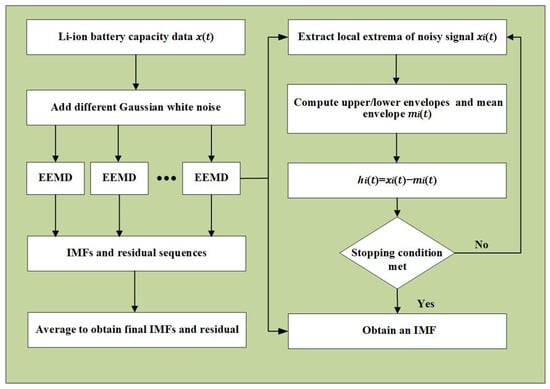
Figure 1. Process of decomposing the aging signal of a lithium-ion battery by EEMD algorithm.

1.

Identify local peaks and local troughs in the sequence $x_i\left(t\right)$, and then use cubic spline interpolation to build the upper envelope $x_{i,max}$ and the lower envelope $x_{i,min}$ from these identified extremes. The mean of these two envelopes is calculated as the mean envelope curve:

$$m_i\left(t\right)={\displaystyle \frac{x_{i,max}\left(t\right)+x_{i,min}\left(t\right)}{2}}$$

(3)

2.

Subtract the mean envelope curve $m_i\left(t\right)$ from the noise-added signal $x_i\left(t\right)$ to generate a new signal $h_i\left(t\right)=x_i\left(t\right)-m_i\left(t\right)$. Next, verify whether the difference between the number of extrema and zero-crossings in $h_i\left(t\right)$ satisfies the stopping criterion (the difference does not exceed 1). If the criterion is met, $h_i\left(t\right)$ is identified as an IMF and denoted as $C_1\left(t\right)$; otherwise, the process is repeated until the IMF condition is satisfied.

3.

Subtract the first extracted IMF component $C_1\left(t\right)$ from the original noise-added signal $x_i\left(t\right)$ to obtain the residual signal. Then, repeat the above procedure on the residual to extract the next-order IMF component. This iterative process continues until the remaining signal satisfies the condition of a monotonic or trend function and can no longer be decomposed into IMFs. The final remaining part is defined as the residual sequence $r_i\left(t\right)$.

Finally, all the IMF components and residual terms obtained from multiple EMD iterations are averaged to derive the final output of the EEMD method. The resulting IMF sequence and residual are computed as

$$C_n\left(t\right)={\displaystyle \frac{1}{N}}\sum _{i=1}^N{C}_{n,i}\left(t\right),R_s\left(t\right)={\displaystyle \frac{1}{N}}\sum _{i=1}^N{r}_i\left(t\right)$$

(4)

2.2. KAN Algorithm

In RUL prediction tasks, accurately modeling the capacity degradation trajectory is crucial for generating high-quality and reliable predictions. To handle the multi-scale and non-stationary aspects of the degradation process, this study initially applies the EEMD technique to decompose the original capacity sequence into multiple IMFs, effectively separating temporal features at different frequency bands. Subsequently, the KAN model is individually constructed for each IMF subsequence to perform targeted modeling and prediction. The predicted components are then aggregated to reconstruct the full capacity degradation curve, enabling accurate estimation of the RUL. The overall modeling framework is illustrated in Figure 2.

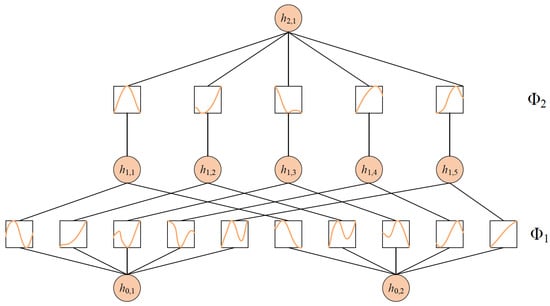
Figure 2. The structure of KAN network.

KAN is a novel neural network grounded in the Kolmogorov–Arnold Representation Theorem. According to this theorem, any multivariate continuous function defined within a finite domain—specifically $f:{[0,1]}^n\to \mathbb{R}$—can be expressed as a finite composition of univariate continuous functions:

$$f(x_1,\dots ,x_n)=\sum _{q=1}^{2n+1}{\mathrm{\Phi }}_q\left(\sum _{p=1}^n{\phi }_{q,p}\left(x_p\right)\right)$$

(5)

where ${\mathrm{\Phi }}_q\in \mathcal{C}(\mathbb{R},\mathbb{R})$ is a composition function located at each node, responsible for aggregating the outputs of multiple univariate functions as input to the next layer. Meanwhile, ${\phi }_{q,p}\in \mathcal{C}([0,1],\mathbb{R})$ represents a univariate activation function defined on each edge, replacing the fixed-weight multiplication used in traditional neural networks.

$${\phi }_{j,i}\left(x\right)=w_b·b\left(x\right)+w_s·spline\left(x\right)$$

(6)

where $b\left(x\right)$ denotes the linear basis function, while $w_b$ and $w_s$ are trainable scaling factors. The term $spline\left(x\right)$ refers to a linear combination based on B-spline basis functions $B_l\left(x\right)$, and is expressed as:

$$spline\left(x\right)=\sum _{l=1}^L{c}_l{B}_l\left(x\right)$$

(7)

where $c_l\in \mathbb{R}$ denotes the learnable spline coefficients, and L represents the number of intervals, reflecting the granularity of the piecewise spline function. A KAN is composed of multiple layers, where the output of each layer is recursively computed as follows:

$$x_{l+1,j}=\sum _{i=1}^{n_l}{\phi }_{l,j,i}\left(x_{l,i}\right)$$

(8)

where ${\phi }_{l,j,i}$ denotes the univariate activation function linked to the connection between the ith node in the l layer and the jth node in the $(l+1)$ layer.

The overall network output function is given by:

$$f\left(x\right)=({\mathrm{\Phi }}_L\circ {\mathrm{\Phi }}_{L-1}\circ \dots \circ {\mathrm{\Phi }}_1)\left(x\right)$$

(9)

where ${\mathrm{\Phi }}^{\left(l\right)}:{\mathbb{R}}^{n_l}\to {\mathbb{R}}^{n_{l+1}}$ denotes the overall transformation function of the l-th layer, mapping from the $n_l$ input nodes to the $n_{l+1}$ output nodes.

In this study, an independent KAN model is constructed for each IMF subsequence to capture its temporal evolution characteristics. The model parameters include spline-based activation functions with learnable scaling coefficients and residual terms, which are optimized using a gradient-based adaptive algorithm during training.

2.3. LSTM Algorithm

LSTM is an advanced variant of recurrent neural networks (RNNs) specifically designed to tackle issues like gradient vanishing and the challenge of capturing long-term dependencies in lengthy sequences. By introducing a cell state and multiple gating mechanisms, LSTM enables selective retention and updating of historical information throughout the sequence.

An LSTM unit comprises three primary gates: forget, input, and output gates, which jointly control the flow of information across time steps, as illustrated in Figure 3.

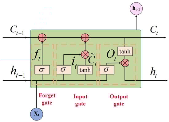
Figure 3. Structure of LSTM unit.

Initially, the forget gate decides whether to retain or discard information from the previous cell state, as described by the following formula:

$$f_t=\sigma (W_f[h_{t-1},x_t]+b_f)$$

(10)

where $f_t$ is the output of the forget gate, $x_t$ denotes the input vector at the current time step, and $h_{t-1}$ is the hidden state from the preceding time step. $W_f$ and $b_f$ represent the weight matrix and bias term, respectively. $\sigma (·)$ is the sigmoid activation function.

Subsequently, the input gate controls how much the current input influences the update of the cell state, which is calculated as

$$i_t=\sigma (W_i[h_{t-1},x_t]+b_i)$$

(11)

$${\tilde{C}}_t=tanh(W_c[h_{t-1},x_t]+b_c)$$

(12)

where $i_t$ denotes the input gate’s output, and ${\tilde{C}}_t$ represents the candidate cell state. $W_i$ and $W_c$ are the corresponding weight matrices, while $b_i$ and $b_c$ are the associated bias terms. $tanh(·)$ denotes the hyperbolic tangent activation function.

The cell state is updated by integrating the outputs from both the forget gate and the input gate, as shown below:

$$C_t=f_t·C_{t-1}+i_t·{\tilde{C}}_t$$

(13)

where $C_t$ denotes the current cell state, and $C_{t-1}$ represents the cell state at the previous time step.

The output gate regulates the generation of the hidden state at the current time step and is computed as follows:

$$o_t=\sigma (W_o[h_{t-1},x_t]+b_o)$$

(14)

$$h_t=o_t·tanh\left(C_t\right)$$

(15)

where $o_t$ denotes the output of the output gate, and $h_t$ represents the hidden state at the current time step. $W_o$ and $b_o$ are the corresponding weight matrix and bias term for the output gate.

Considering the ability of LSTM networks to integrate both current input and historical states in time series modeling, they are well-suited for constructing regression models with temporal dependencies and capturing nonlinear dynamic features. To precisely capture the degradation trend of lithium-ion battery RUL over time, the raw capacity sequence is initially processed through EEMD to isolate the residual component. The extracted residual sequence is subsequently provided as input to the LSTM model, allowing the training of a dedicated predictor to model and forecast complex, nonstationary degradation dynamics. The overall procedure is illustrated as follows:

1.

The residual sequence is divided into training and testing sets in a 1:1 ratio for model training and performance evaluation.

2.

The cycle index functions as the model input, while the corresponding residual value serves as the prediction target. An LSTM network is built using the training data to learn and fit the residual sequence.

3.

The cycle indices from the testing subset are subsequently input into the trained LSTM model to generate the predicted residual sequence, which is used to assess the model’s generalization capability on unseen data.

In the context of RUL prediction for lithium-ion batteries, the cell state retains latent dependencies between the input sequence and the prediction target, effectively capturing long-term correlations between the cycle index and residual data. The forget gate manages the retention of information from the preceding cell state, thus controlling the decay of past memory. The input gate not only generates the candidate state at the current time step but also determines—through a gating signal—whether this information should be incorporated into the cell state, enabling dynamic updates of the hidden representation. Finally, the output gate combines the current cell state with control signals to produce the hidden state for the current time step, which is subsequently employed to predict the residual sequence.

3. Experimental Data and RUL Prediction Framework

3.1. Experimental Data

To verify the proposed method’s effectiveness, this study utilizes an accelerated aging dataset of lithium-ion batteries supplied by NASA. Three experimental sequences, labeled B05, B06, and B18, are specifically selected for analysis, as shown in Figure 4a. The tested cells are of type LiNi_0.8Co_0.15Al_0.05O₂ with a nominal capacity of 2 Ah. Although all three batteries follow the same test protocol, their degradation trajectories and service lifespans vary due to differences in initial health conditions. Among them, B05 and B18 exhibit more pronounced capacity degradation, while B06 shows relatively stable behavior. In this work, the failure threshold for RUL estimation is set at 70% of the initial nominal capacity.

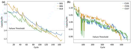
Figure 4. Experimental raw data of (a) B05, B06 and B18 and (b) CS35, CS36 and CS37.

This study utilized aging data for lithium-ion batteries CS35, CS36, and CS37, obtained from the CALCE laboratory, as illustrated in Figure 4b. The battery cells tested are LiCoO₂ with a nominal capacity of 1.1 Ah. Compared to B05, B06, and B18, these cells were subjected to different experimental conditions. Specifically, cell CS was operated under a distinct aging protocol. To assess the influence of varying failure threshold settings on the proposed RUL prediction approach, the failure threshold for the CS series batteries is set at 80% of their initial nominal capacity.

3.2. Lithium-Ion Battery RUL Prediction Workflow

Due to the intrinsic electrochemical nature of lithium-ion batteries and the considerable uncertainties in their operating conditions, observed aging data often exhibit significant capacity regeneration and pronounced nonlinear behavior. These characteristics complicate RUL prediction, particularly in identifying degradation patterns within the prediction horizon, which is critical for achieving reliable model performance. However, directly using raw aging sequences—characterized by nonlinear fluctuations and regeneration effects—as training data can hinder the development of stable and generalizable prediction models. To improve prediction accuracy, this study employs the EEMD method to decompose the original aging sequence into multiple IMFs and a residual component. The residual sequence primarily captures the long-term degradation trajectory of the battery, which exhibits overall smoothness and a consistent upward or downward trend. In contrast, the IMFs contain higher-frequency components that reflect regeneration behavior and external measurement noise, thereby isolating nonstationary factors for targeted modeling.

Based on this decomposition strategy, separate prediction models are constructed for the IMFs and the residual component. The individual predictions are then fused to estimate the battery’s RUL. Figure 5 presents the full prediction process, and the following sections provide a detailed explanation of each step.

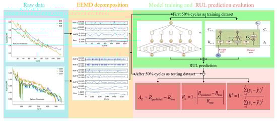
Figure 5. Workflow of RUL prediction.

1. The EEMD algorithm is applied to the nonlinear discharge capacity sequence, yielding several IMFs and one residual sequence. The residual sequence primarily reflects the long-term degradation trend, while the IMFs capture regeneration behavior and measurement noise.

2. The residual and IMF sequences are divided into training and testing subsets in a 1:1 ratio for model training and validation.

3. For the residual sequence, the charge–discharge cycle count is used as the input feature, with the corresponding residual values as prediction targets. An LSTM network is then trained to model and forecast the residual sequence.

4. For the IMF components, the cycle count again serves as the input, while the corresponding IMF values act as targets. A KAN model is constructed to individually forecast each IMF sequence.

5. The trained LSTM and KAN models are subsequently employed to generate 294 predictions for the residual sequence and IMF components corresponding to the testing 295 cycles.

6. The predicted residual and IMF components are aggregated at each cycle to reconstruct the battery’s discharge capacity trajectory.

4. Experimental Results and Discussion

Figure 6 and Figure 7 show the IMFs and residual components extracted via EEMD from the battery degradation data in the NASA and Maryland datasets. Due to the adaptive nature of the EEMD algorithm, the decomposition process terminates once the residual evolves into a monotonic function. As a result, the number of extracted IMFs varies across different battery samples such as B05, B06, and B18. The decomposition results indicate that the residual component predominantly represents the long-term degradation trend in battery capacity, whereas the individual IMFs capture localized oscillatory patterns in the original signal, mainly associated with capacity regeneration effects and high-frequency noise from measurements.

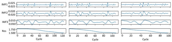
Figure 6. EEMDdecomposition results of B05, B06 and B18.

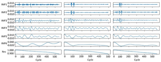
Figure 7. EEMD decomposition results of CS35, CS36 and CS37.

The proposed method employs LSTM and KAN models to separately predict the residual sequence and the IMF components obtained via EEMD decomposition. The predictions for each individual will then be combined to reconstruct the expected decay pattern of lithium-ion battery discharge capacity over time, allowing for additional estimates of its RUL. To quantitatively evaluate the effectiveness of the proposed approach in RUL prediction, absolute error (AE) and relative accuracy (RA) are introduced as the primary evaluation metrics. These metrics reflect the deviation between predicted and actual RUL values, and the relative precision of the predictions, respectively. In addition, to assess the goodness-of-fit between the predicted capacity trajectory and the actual degradation curve, the coefficient of determination ($R^2$) is adopted. A higher $R^2$ value—closer to 1—indicates a stronger correlation between the predicted results and the ground truth. The definitions of AE, RA, and $R^2$ are given as follows:

$$A_E=R_{\mathrm{predicted}}-R_{\mathrm{true}}$$

(16)

$$R_A=1-\left|{\displaystyle \frac{R_{\mathrm{predicted}}-R_{\mathrm{true}}}{R_{\mathrm{true}}}}\right|$$

(17)

$$R^2=1-{\displaystyle \frac{{\displaystyle \sum _{i=1}^n}{(y_i-{\widehat{y}}_i)}^2}{{\displaystyle \sum _{i=1}^n}{(y_i-{\overline{y}}_i)}^2}}$$

(18)

where $R_{\mathrm{predicted}}$ and $R_{\mathrm{true}}$ denote the predicted and actual RUL, respectively; n represents the number of charge–discharge cycles; y refers to the measured discharge capacity sequence, and $\widehat{y}$ is the corresponding sequence predicted by the model.

To further quantify the magnitude of deviation between the predicted and actual values, the root mean square error (RMSE) is also introduced as a supplementary metric:

$$\mathrm{RMSE}=\sqrt{{\displaystyle \frac{1}{n}}\sum _{i=1}^n{(y_i-{\widehat{y}}_i)}^2}$$

(19)

On the three representative battery samples from the NASA dataset—B05, B06, and B18—the proposed KAN-LSTM model demonstrates outstanding predictive performance. As shown in Figure 8, the predicted capacity curves closely follow the actual capacity degradation trends, with no significant deviations or lag observed. Even in challenging cases such as B18, where notable capacity regeneration and other non-stationary behaviors are present, the model maintains strong robustness and accurate fitting performance. In terms of quantitative evaluation, as reported in Table 1, the $R^2$ exceeds 0.95 for all three samples, indicating that the model effectively captures the underlying degradation dynamics. The RA is also consistently above 0.95, suggesting high consistency in cycle-wise alignment. Furthermore, the absolute error in RUL prediction is controlled within a narrow range of 2 to 3 charge–discharge cycles.

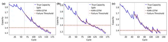
Figure 8. RUL prediction results of (a) B05 (b) B06 and (c) B18.

Table 1. Comparison results of KAN-LSTM on NASA datasets.

Metric	B05				B06				B18
	AE	RA	${\mathit{R}}^{\mathbf{2}}$	RMSE	AE	RA	${\mathit{R}}^{\mathbf{2}}$	RMSE	AE	RA	${\mathit{R}}^{\mathbf{2}}$	RMSE
KAN-LSTM	3	0.9523	0.9611	0.0159	2	0.9636	0.9534	0.0169	2	0.9592	0.9706	0.0158

For the CS35, CS36, and CS37 battery datasets from the CALCE benchmark, the KAN-LSTM model effectively adapts to longer degradation cycles and more complex fluctuation patterns. As illustrated in Figure 9 and detailed in Table 2, the predicted capacity curves exhibit overall trends that closely match the actual degradation trajectories, successfully capturing the nonlinear aging behavior of the batteries. Despite the presence of measurement noise and temporary capacity recovery in certain samples, the model demonstrates strong stability and robustness against disturbances. All three battery samples achieve $R^2$ values exceeding 0.91, indicating high regression accuracy over the full lifespan. The RA values are all above 0.93, confirming that the predicted RUL closely aligns with the actual failure point. Notably, CS37 achieves the highest RA, approaching 0.98, which reflects excellent prediction precision. Furthermore, the absolute prediction errors remain within a reasonable range across all samples, with the maximum deviation not exceeding 15 cycles. No systematic overestimation or underestimation trends were observed, further validating the reliability of proposed method.

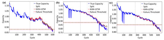
Figure 9. RUL prediction results of (a) CS35 (b) CS36 and (c) CS37.

Table 2. Comparison results of KAN-LSTM on CALCE datasets.

Metric	C35				C36				C37
	AE	RA	${\mathit{R}}^{\mathbf{2}}$	RMSE	AE	RA	${\mathit{R}}^{\mathbf{2}}$	RMSE	AE	RA	${\mathit{R}}^{\mathbf{2}}$	RMSE
KAN-LSTM	12	0.9567	0.9111	0.0086	15	0.9398	0.9333	0.0099	−7	0.9752	0.9104	0.0071

Furthermore, four models—GRU, LSTM, KAN, and the proposed KAN-LSTM—were selected for comparative experiments. Figure 10 and Table 3 present the fitting results of each model for the capacity degradation trajectories. The GRU and LSTM, as two mainstream recurrent neural network architectures, exhibit noticeable fitting errors and trend shifts in most samples. In particular, they tend to underestimate or overestimate the capacity during later degradation stages, resulting in relatively lower RA and $R^2$ values. The KAN model, constructed based on the Kolmogorov–-Arnold representation theorem, outperforms both GRU and LSTM across all three samples, demonstrating stronger nonlinear modeling capability. Its $R^2$ values consistently exceed 0.90, and the RA scores range from 0.89 to 0.93, indicating good overall fitting performance. However, when used alone, the KAN model shows delayed responses in certain high-frequency fluctuation regions, leading to slightly lower prediction accuracy compared to the proposed hybrid model. By incorporating the temporal dependency modeling strength of LSTM, the KAN-LSTM model achieves superior performance across all evaluation metrics in the three samples. It produces the lowest AE and consistently attains RA and $R^2$ values above 0.95.

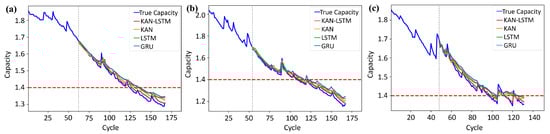
Figure 10. Comparisonof RUL prediction results of (a) B05 (b) B06 and (c) B18.

Table 3. Comparison of the proposed algorithm with other methods on NASA.

Case	Metric	GRU	LSTM	KAN	KAN-LSTM
B05	AE	13	11	6	3
	RA	0.7936	0.8254	0.9048	0.9523
	$R^2$	0.9029	0.9135	0.9477	0.9611
	RMSE	0.0251	0.0237	0.0184	0.0159
B06	AE	8	7	4	2
	RA	0.8545	0.8727	0.9273	0.9636
	$R^2$	0.8628	0.8778	0.9007	0.9534
	RMSE	0.0291	0.0274	0.0247	0.0169
B18	AE	8	7	5	2
	RA	0.8367	0.8571	0.8980	0.9592
	$R^2$	0.8612	0.9117	0.9259	0.9706
	RMSE	0.0387	0.0226	0.0170	0.0158

Similarly, the comparative results on the CALCE datasets are shown in Figure 11 and Table 4. The KAN-LSTM model consistently demonstrates the best overall performance in terms of prediction accuracy and fitting capability. Its $R^2$ values all exceed 0.91, and its RA values are consistently higher than those of the other models, indicating that it can accurately reconstruct the capacity degradation trend and effectively identify the failure cycle. However, for the CS37 sample, the KAN-LSTM model exhibits an absolute error of −7, with the predicted trajectory slightly underestimating the actual capacity across the lifespan. In comparison, the KAN model also outperforms both GRU and LSTM across all three CALCE samples. Its RA values remain above 0.91, and $R^2$ scores are close to 0.90, reflecting strong nonlinear modeling capabilities. Nevertheless, due to its limited ability to capture temporal dependencies, the KAN model shows slightly weaker local fitting performance near the end-of-life (EOL) region compared to the KAN-LSTM model. The GRU and LSTM models perform less satisfactorily on the datasets. In particular, for the CS35 and CS37 samples, the absolute errors reach as high as 23/38 and −24/24 cycles, respectively. Their $R^2$ values generally fall below 0.83, and their fitting curves exhibit significant trend deviations, with evident overestimation or insufficient responsiveness to high-frequency fluctuations.

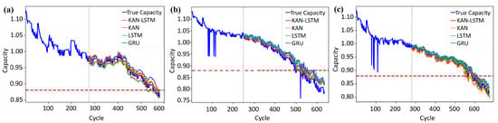
Figure 11. Comparison of RUL prediction results of (a) CS35 (b) CS36 and (c) CS37.

Table 4. Comparison of the proposed algorithm with other methods on CALCE.

Case	Metric	GRU	LSTM	KAN	KAN-LSTM
C35	AE	23	−24	22	12
	RA	0.9170	0.9134	0.9206	0.9567
	$R^2$	0.7524	0.8084	0.9053	0.9111
	RMSE	0.0143	0.0126	0.0089	0.0086
C36	AE	34	23	22	15
	RA	0.8635	0.9076	0.9116	0.9398
	$R^2$	0.8037	0.8229	0.9001	0.9333
	RMSE	0.0169	0.0161	0.0121	0.0099
C37	AE	38	24	−15	−7
	RA	0.8657	0.9152	0.9470	0.9752
	$R^2$	0.7544	0.8300	0.8326	0.9104
	RMSE	0.0117	0.0097	0.0097	0.0071

Therefore, while the KAN model demonstrates strong fitting performance owing to its structural advantages, its integration with LSTM enables a more effective exploitation of complementary strengths. The KAN-LSTM model combines the powerful nonlinear function approximation capability of KAN with the temporal dependency modeling strength of LSTM, thereby achieving more accurate and robust modeling of the complex degradation processes.

To explore the modeling capabilities of the KAN model across different frequency components and its parameter adaptation strategies, a systematic analysis was conducted on multiple battery samples from the NASA and CALCE datasets. Specifically, the optimal hyperparameter configurations for each IMF component were extracted, with a focus on examining the relationship between the hidden layer dimension (Dim), the number of interval partitions per input variable (G), the order of the spline functions (K), and the model’s prediction performance measured by RMSE.

The optimal hyperparameter ranges of the KAN model for different frequency IMF components are summarized in Table 5. In the CALCE datasets, IMF1–IMF3 typically represent high-frequency disturbances or localized rapid oscillations, characterized by significant variations and complex structures. Therefore, higher network capacity is required to achieve accurate fitting. The optimal configurations for these components generally fall within the ranges of Dim = 128–256, G = 6–8, and K = 5–7. In contrast, IMF4 and IMF5 often correspond to mid-frequency or periodic components with more stable structures, demanding moderate model complexity. Their optimal parameters are mostly found in Dim = 64–128, G = 4–6, and K = 3–5. As for IMF6, which captures long-term capacity degradation trends as the lowest frequency component, satisfactory performance with extremely low RMSE can be achieved using lightweight settings such as Dim = 64, G = 3–5, and K = 2–3. This also results in significantly faster training and better modeling stability. Furthermore, a similar pattern is observed in the analysis of the NASA datasets. In terms of frequency characteristics, IMF1 from NASA shows strong consistency with IMF1–IMF3 from CALCE, exhibiting pronounced high-frequency disturbances. Meanwhile, NASA’s IMF2 and IMF3 resemble CALCE’s IMF4 and IMF5, primarily capturing periodic trends. The corresponding optimal hyperparameters are also found to concentrate around Dim = 128, G = 4–6, and K = 2–4, aligning well with those in the CALCE datasets. Although Dim = 128 yields the best RMSE in NASA’s IMF2 and IMF3, performance with Dim = 64 remains only marginally lower, indicating that the IMF-specific parameter setting strategy proposed in this study demonstrates strong transferability and generalization across different datasets.

Table 5. Optimal KAN hyperparameter configurations for different IMF components across NASA and CALCE datasets.

B05					B06					B18
IMF	Dim	G	K	RMSE	IMF	Dim	G	K	RMSE	IMF	Dim	G	K	RMSE
IMF1	128	6	2	0.0071	IMF1	256	6	2	0.0120	IMF1	128	6	5	0.0105
IMF2	128	6	4	0.0062	IMF2	128	5	2	0.0102	IMF2	128	6	7	0.0059
IMF3	128	3	2	0.0057	IMF3	64	6	5	0.0101	IMF3	64	4	2	0.0104
CS35					CS36					CS37
IMF1	128	7	6	0.0024	IMF1	256	7	4	0.0027	IMF1	256	7	4	0.0025
IMF2	128	7	6	0.0025	IMF2	256	5	5	0.0026	IMF2	128	5	5	0.0025
IMF3	128	4	6	0.0018	IMF3	128	4	5	0.0022	IMF3	128	4	5	0.0017
IMF4	64	7	4	0.0021	IMF4	64	7	3	0.0024	IMF4	64	7	2	0.0018
IMF5	64	5	2	0.0013	IMF5	64	7	2	0.0012	IMF5	64	5	2	0.0009
IMF6	64	3	3	0.0018	IMF6	128	6	7	0.0030	IMF6	64	7	3	0.0005

5. Conclusions

This paper proposes a hybrid RUL prediction framework based on EEMD, LSTM, and KAN to model complex battery degradation behaviors. Experimental results on NASA and CALCE datasets demonstrate that the proposed KAN-LSTM model outperforms conventional LSTM, GRU, and standalone KAN approaches, achieving higher prediction accuracy and stronger robustness under varying degradation scenarios. The average $R^2$ exceeds 0.96 on the NASA dataset and remains above 0.91 on CALCE, with RUL errors within acceptable ranges. In addition, optimal KAN hyperparameters for different IMF components are identified, offering practical guidance for future multi-scale modeling. This framework holds promise for integration into battery management systems or cloud-based diagnostics, enabling more accurate health assessment and predictive maintenance in real-world energy storage applications.

References

- Aljohani, A.; Aljohani, S. A Hybrid GRU-MHA model for accurate battery RUL forecasting with feature selection. Energy Rep. 2025, 14, 294–309. [Google Scholar] [CrossRef]
- Cao, J.; Harrold, D.; Fan, Z.; Morstyn, T.; Healey, D.; Li, K. Deep reinforcement learning-based energy storage arbitrage with accurate lithium-ion battery degradation model. IEEE Trans. Smart Grid 2020, 11, 4513–4521. [Google Scholar] [CrossRef]
- Ding, X.; Wang, Z.; Zhang, L.; Wang, C. Longitudinal vehicle speed estimation for four-wheel-independently-actuated electric vehicles based on multi-sensor fusion. IEEE Trans. Veh. Technol. 2020, 69, 12797–12806. [Google Scholar] [CrossRef]
- Zhang, L.; Hu, X.; Wang, Z.; Sun, F.; Deng, J.; Dorrell, D.G. Multiobjective optimal sizing of hybrid energy storage system for electric vehicles. IEEE Trans. Veh. Technol. 2017, 67, 1027–1035. [Google Scholar] [CrossRef]
- Zhang, C.; Tu, L.; Yang, Z.; Du, B.; Zhou, Z.; Wu, J.; Chen, L. A CMMOG-based lithium-battery SOH estimation method using multi-task learning framework. J. Energy Storage 2025, 107, 114884. [Google Scholar] [CrossRef]
- Eto, A.; Akimoto, Y.; Okajima, K.; Okano, J.; Onoue, Y. Evaluation of lithium-ion batteries with different structures using magnetic field measurement for onboard battery identification. Glob. Energy Interconnect. 2025, 10, 100257. [Google Scholar] [CrossRef]
- Li, R.; Kirkaldy, N.D.; Oehler, F.F.; Marinescu, M.; Offer, G.J.; O’Kane, S.E.J. The importance of degradation mode analysis in parameterising lifetime prediction models of lithium-ion battery degradation. Nat. Commun. 2025, 16, 2776. [Google Scholar] [CrossRef]
- Zraibi, B.; Okar, C.; Chaoui, H.; Mansouri, M. Remaining Useful Life Assessment for Lithium-Ion Batteries Using CNN-LSTM-DNN Hybrid Method. IEEE Trans. Veh. Technol. 2021, 70, 4252–4261. [Google Scholar] [CrossRef]
- Mejdoubi, A.; Chaoui, H.; Gualous, H. Lithium-ion batteries health prognosis considering aging conditions. IEEE Trans. Power Electron. 2019, 34, 6834–6844. [Google Scholar] [CrossRef]
- Zhang, C.; Luo, L.; Yang, Z.; Zhao, S.; He, Y.; Wang, X.; Wang, H. Battery SOH estimation method based on gradual decreasing current, double correlation analysis and GRU. Green Energy Intell. Transp. 2023, 2, 100108. [Google Scholar] [CrossRef]
- Chen, L.; Lopes, A.M.; Xie, S.; Li, H.; Bao, X.; Zhang, C.; Li, P. A new SOH estimation method for Lithium-ion batteries based on model-data-fusion. Energy 2023, 286, 129597. [Google Scholar] [CrossRef]
- Guo, X.; Wang, K.; Yao, S.; Fu, G.; Ning, Y. RUL prediction of lithium ion battery based on CEEMDAN-CNN BiLSTM model. Energy Rep. 2023, 9, 1299–1306. [Google Scholar] [CrossRef]
- Cadini, F.; Sbarufatti, C.; Cancelliere, F.; Giglio, M. State-of-life prognosis and diagnosis of lithium-ion batteries by data-driven particle filters. Appl. Energy 2019, 235, 661–672. [Google Scholar] [CrossRef]
- Lee, S.; Han, S.; Han, K.H.; Kim, Y.; Agarwal, S.; Hariharan, K.S.; Oh, B.; Yoon, J. Diagnosing various failures of lithium-ion batteries using artificial neural network enhanced by likelihood mapping. J. Energy Storage 2021, 40, 102768. [Google Scholar] [CrossRef]
- Tang, X.; Liu, K.; Li, K.; Widanage, W.D.; Kendrick, E.; Gao, F. Recovering large-scale battery aging dataset with machine learning. Patterns 2021, 2, 100302. [Google Scholar] [CrossRef]
- Zhang, C.; Zhao, S.; He, Y. An integrated method of the future capacity and RUL prediction for lithium-ion battery pack. IEEE Trans. Veh. Technol. 2021, 71, 2601–2613. [Google Scholar] [CrossRef]
- Bao, X.; Chen, L.; Lopes, A.M.; Li, X.; Xie, S.; Li, P.; Chen, Y. Hybrid deep neural network with dimension attention for state-of-health estimation of Lithium-ion Batteries. Energy 2023, 278, 127734. [Google Scholar]
- Gao, K.; Xu, J.; Li, Z.; Cai, Z.; Jiang, D.; Zeng, A. A Novel Remaining Useful Life Prediction Method for Capacity Diving Lithium-Ion Batteries. ACS Omega 2022, 7, 26701–26714. [Google Scholar] [CrossRef]
- Shrivastava, P.; Naidu, P.A.; Sharma, S.; Panigrahi, B.K.; Garg, A. Review on technological advancement of lithium-ion battery states estimation methods for electric vehicle applications. J. Energy Storage 2023, 69, 107159. [Google Scholar] [CrossRef]
- Pang, H.; Chen, K.; Geng, Y.; Wu, L.; Wang, F.; Liu, J. Accurate capacity and remaining useful life prediction of lithium-ion batteries based on improved particle swarm optimization and particle filter. Energy 2024, 293, 130555. [Google Scholar] [CrossRef]
- Madani, S.S.; Shabeer, Y.; Allard, F.; Fowler, M.; Ziebert, C.; Wang, Z.; Panchal, S.; Chaoui, H.; Mekhilef, S.; Dou, S.X.; et al. A Comprehensive Review on Lithium-Ion Battery Lifetime Prediction and Aging Mechanism Analysis. Batteries 2025, 11, 127. [Google Scholar] [CrossRef]
- Ahwiadi, M.; Wang, W. An AI-Driven Particle Filter Technology for Battery System State Estimation and RUL Prediction. Batteries 2024, 10, 437. [Google Scholar] [CrossRef]
- Li, X.; Yuan, C.; Wang, Z.; Xie, J. A data-fusion framework for lithium battery health condition Estimation Based on differential thermal voltammetry. Energy 2022, 239, 122206. [Google Scholar] [CrossRef]
- Guo, F.; Wu, X.; Liu, L.; Ye, J.; Wang, T.; Fu, L.; Wu, Y. Prediction of remaining useful life and state of health of lithium batteries based on time series feature and Savitzky-Golay filter combined with gated recurrent unit neural network. Energy 2023, 270, 126880. [Google Scholar] [CrossRef]
- Wu, C.; Xu, C.; Wang, L.; Fu, J.; Meng, J. Lithium-ion battery remaining useful life prediction based on data-driven and particle filter fusion model. Green Energy Intell. Transp. 2025, 2, 100267. [Google Scholar] [CrossRef]
- Chen, Y.; Duan, W.; He, Y.; Wang, S.; Fernandez, C. A hybrid data driven framework considering feature extraction for battery state of health estimation and remaining useful life prediction. Green Energy Intell. Transp. 2024, 1, 100160. [Google Scholar] [CrossRef]
- Wang, C.; Wang, R.; Li, J.; Li, Z.; Yu, Q. Cycle-Efficient modeling for degradation staging and early life prediction of lithium batteries. Green Energy Intell. Transp. 2025, 2, 100338. [Google Scholar] [CrossRef]
- Olabi, A.G.; Abbas, Q.; Shinde, P.A.; Abdelkareem, M.A. Rechargeable batteries: Technological advancement, challenges, current and emerging applications. Energy 2022, 254, 126408. [Google Scholar] [CrossRef]
- Reza, M.; Hannan, M.; Mansor, M.; Ker, P.J.; Rahman, S.; Jang, G.; Mahlia, T.I. Towards enhanced remaining useful life prediction of lithium-ion batteries with uncertainty using optimized deep learning algorithm. J. Energy Storage 2024, 98, 113056. [Google Scholar] [CrossRef]
- Tian, J.; Xu, R.; Wang, Y.; Chen, Z. Capacity attenuation mechanism modeling and health assessment of lithium-ion batteries. Energy 2021, 221, 119682. [Google Scholar] [CrossRef]
- Ahwiadi, M.; Wang, W. An enhanced particle filter technology for battery system state estimation and RUL prediction. Measurement 2022, 191, 110817. [Google Scholar] [CrossRef]
- Hong, S.; Qin, C.; Lai, X.; Meng, Z.; Dai, H. State-of-health estimation and remaining useful life prediction for lithium-ion batteries based on an improved particle filter algorithm. J. Energy Storage 2023, 64, 107179. [Google Scholar] [CrossRef]
- Qiu, X.; Wu, W.; Wang, S. Remaining useful life prediction of lithium-ion battery based on improved cuckoo search particle filter and a novel state of charge estimation method. J. Power Sources 2020, 450, 227700. [Google Scholar] [CrossRef]
- Sun, X.; Zhong, K.; Han, M. A hybrid prognostic strategy with unscented particle filter and optimized multiple kernel relevance vector machine for lithium-ion battery. Measurement 2021, 170, 108679. [Google Scholar] [CrossRef]
- Chen, L.; An, J.; Wang, H.; Zhang, M.; Pan, H. Remaining useful life prediction for lithium-ion battery by combining an improved particle filter with sliding-window gray model. Energy Rep. 2020, 6, 2086–2093. [Google Scholar] [CrossRef]
- Yang, J.; Fang, W.; Chen, J.; Yao, B. A lithium-ion battery remaining useful life prediction method based on unscented particle filter and optimal combination strategy. J. Energy Storage 2022, 55, 105648. [Google Scholar] [CrossRef]
- Zheng, Z.; Zhao, G.; Yang, J.; Zhao, Z.; Gao, J. The reutilization screening of retired electric vehicle lithium-ion battery based on coulombic efficiency. Trans. China Electrotech. Soc. 2019, 34, 388–395. [Google Scholar]
- Lai, X.; Jin, C.; Yi, W.; Han, X.; Feng, X.; Zheng, Y.; Ouyang, M. Mechanism, modeling, detection, and prevention of the internal short circuit in lithium-ion batteries: Recent advances and perspectives. Energy Storage Mater. 2021, 35, 470–499. [Google Scholar] [CrossRef]
- Li, X.; Yuan, C.; Li, X.; Wang, Z. State of health estimation for Li-Ion battery using incremental capacity analysis and Gaussian process regression. Energy 2020, 190, 116467. [Google Scholar] [CrossRef]
- Ren, L.; Dong, J.; Wang, X.; Meng, Z.; Zhao, L.; Deen, M.J. A data-driven auto-CNN-LSTM prediction model for lithium-ion battery remaining useful life. IEEE Trans. Ind. Inform. 2020, 17, 3478–3487. [Google Scholar] [CrossRef]
- Yang, Z.; Wang, Y.; Kong, C. Remaining useful life prediction of lithium-ion batteries based on a mixture of ensemble empirical mode decomposition and GWO-SVR model. IEEE Trans. Instrum. Meas. 2021, 70, 2517011. [Google Scholar] [CrossRef]
- Kong, J.z.; Yang, F.; Zhang, X.; Pan, E.; Peng, Z.; Wang, D. Voltage-temperature health feature extraction to improve prognostics and health management of lithium-ion batteries. Energy 2021, 223, 120114. [Google Scholar] [CrossRef]
- Pang, X.; Liu, X.; Jia, J.; Wen, J.; Shi, Y.; Zeng, J.; Zhao, Z. A lithium-ion battery remaining useful life prediction method based on the incremental capacity analysis and Gaussian process regression. Microelectron. Reliab. 2021, 127, 114405. [Google Scholar] [CrossRef]
- Zhang, Y.; Xiong, R.; He, H.; Pecht, M.G. Long short-term memory recurrent neural network for remaining useful life prediction of lithium-ion batteries. IEEE Trans. Veh. Technol. 2018, 67, 5695–5705. [Google Scholar] [CrossRef]
- Tong, Z.; Miao, J.; Tong, S.; Lu, Y. Early prediction of remaining useful life for Lithium-ion batteries based on a hybrid machine learning method. J. Clean. Prod. 2021, 317, 128265. [Google Scholar] [CrossRef]
- Cheng, G.; Wang, X.; He, Y. Remaining useful life and state of health prediction for lithium batteries based on empirical mode decomposition and a long and short memory neural network. Energy 2021, 232, 121022. [Google Scholar] [CrossRef]
- He, Y.; Wang, Y. Short-term wind power prediction based on EEMD–LASSO–QRNN model. Appl. Soft Comput. 2021, 105, 107288. [Google Scholar] [CrossRef]
- Li, H.; Liu, T.; Wu, X.; Li, S. Research on test bench bearing fault diagnosis of improved EEMD based on improved adaptive resonance technology. Measurement 2021, 185, 109986. [Google Scholar] [CrossRef]
Disclaimer/Publisher’s Note: The statements, opinions and data contained in all publications are solely those of the individual author(s) and contributor(s) and not of MDPI and/or the editor(s). MDPI and/or the editor(s) disclaim responsibility for any injury to people or property resulting from any ideas, methods, instructions or products referred to in the content. |
© 2025 by the authors. Licensee MDPI, Basel, Switzerland. This article is an open access article distributed under the terms and conditions of the Creative Commons Attribution (CC BY) license (https://creativecommons.org/licenses/by/4.0/).