Abstract
Precision monitoring of leaf nitrogen content (LNC) in fruit trees is critical for optimizing fertilization and fruit quality. In this study, 1120 apple-leaf samples spanning two phenological stages were collected. Characteristic wavelengths were selected using competitive adaptive reweighted sampling and the successive projection algorithm (CARS–SPA). To mitigate inefficient exploration during population initialization and iterations, we propose a collaborative enhancement strategy integrating Sobol-sequence sampling and elite opposition-based learning (EOBL), termed SEO, which simultaneously refines initialization and iterative updating in swarm-based optimization algorithms. Four machine learning algorithms were trained to construct cross-phenological-stage LNC inversion models. Results indicated characteristic wavelengths lay within the visible region. The combined SEO strategy improved search capability and efficiency, with SEO-BKA achieving the best performance. Consequently, the SEO-BKA-XGBoost model yielded the highest accuracy in the bloom and fruit-set stage (R2 = 0.883; RMSE = 0.124) and fruit-enlargement stage (R2 = 0.897; RMSE = 0.069). These findings provide robust technical support for LNC hyperspectral inversion in apple trees.
1. Introduction
The apple is one of the most economically important fruit crops and a valuable component of a balanced diet, with regular consumption being linked to immune support and a lower risk of chronic diseases [1]. With ongoing population growth and rapid economic development, increasing fruit production to meet rising market demand has become an urgent priority [2]. Nitrogen, as one of the essential nutrients for plant growth and development, plays a critical role in the physiological metabolism of apple trees. It directly participates in chlorophyll synthesis, protein formation, and nucleic acid biosynthesis, and its effects are readily reflected in fruit size, external appearance, and yield [3]. However, in commercial orchard production, growers often apply excessive nitrogen fertilizer in an attempt to increase yield. Nitrogen oversupply disrupts the metabolic and physiological balance of apple trees, reduces leaf photosynthetic efficiency, suppresses vegetative growth, impairs reproductive development and flower bud differentiation, decreases fruit set, and ultimately degrades fruit quality [4]. Conversely, nitrogen deficiency also has negative effects on fruit trees: leaves become smaller and chlorotic, photosynthetic capacity weakens, pest and disease resistance decreases, fruit yield declines, and premature senescence or even mortality of trees may be accelerated [5]. Therefore, monitoring nitrogen status and maintaining an appropriate nitrogen balance are essential for healthy growth and development of apple trees.
Conventional chemical reagent-based analysis provides high accuracy, but it typically requires destructive processing of plant tissues, involves complex laboratory procedures, and is not suitable for large-scale implementation in orchards [6]. In recent years, spectroscopic techniques, owing to their non-destructive and non-contact characteristics, have been widely applied for monitoring vegetation growth, diagnosing pest and disease infestations, and assessing water quality and soil nutrient status [7,8]. To extract nitrogen-related characteristic wavelengths from large volumes of hyperspectral reflectance data and to reduce data redundancy and multicollinearity, many studies have adopted variable selection methods to construct a compact and informative feature subset, remove redundant, irrelevant, or misleading variables, thereby improving the predictive performance of the regression model [9,10,11]. Using the constructed subset of characteristic variables, regression modeling can be applied to estimate LNC. Machine learning algorithms do not rely on strict probabilistic distribution assumptions; instead, they learn relationships directly from data. These algorithms perform well when handling high-dimensional, nonlinear datasets and have already been used to detect physiological and biochemical parameters of fruit trees, including chlorophyll content, nitrogen content, and water content [12,13,14].
Appropriate configuration of machine learning model hyperparameters is fundamental for ensuring model efficiency, and numerous studies have focused on algorithms for hyperparameter optimization. Wei Luo et al. (2025) integrated a global search whale optimization algorithm (GSWOA) with a kernel extreme learning machine (KELM), This integration significantly substantially improved the prediction accuracy of catechin content in green tea [15]. Zhen Qin et al. (2024) combined Bayesian optimization (BO), particle swarm optimization (PSO), genetic algorithms (GA), and simulated annealing (SA) to optimize random forest (RF), XGBoost, and support vector regression (SVR) models, and reported that the BO-GBRT model outperformed conventional methods in both accuracy and stability [16]. Kapil Khandelwal et al. (2025) investigated hydrogen yield in the supercritical water gasification of biomass and systematically compared genetic algorithms and PSO across eight machine learning models; their results indicated that the PSO-XGBoost combination achieved the highest predictive performance [17].
Taken together, previous studies have shown that swarm-based optimization algorithms, which simulate cooperative, competitive, and foraging behaviors in biological populations and exploit information exchange and feedback among individuals, are highly competitive in terms of global search capability and computational efficiency. However, most existing swarm-based optimization algorithms still employ random population initialization. Although random initialization can increase population diversity to some extent, it often results in non-uniform sampling in high-dimensional search spaces, which can in turn induce premature convergence.
This study aims to develop a hyperspectral inversion model for LNC. To this end, we propose an enhanced swarm-based optimization strategy, termed SEO, that integrates Sobol-sequence sampling with elite opposition-based learning (EOBL) to optimize the hyperparameters of machine-learning regression models, thereby enabling accurate and non-destructive estimation of LNC in apple leaves. The flowchart of the research methodology is shown in Figure 1. The specific objectives of this study are as follows:
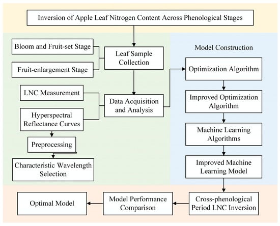
Figure 1.
Flowchart of the research methodology. This figure presents the overall research framework, including sample collection, measurement of LNC and spectral curves, and model development. Notably, the model construction process involves the enhancement of optimization algorithms and the application of machine learning models.
(a) To acquire hyperspectral reflectance curves from apple leaves and, using spectral feature selection methods, identify the characteristic wavelengths in the leaf reflectance spectrum that are associated with nitrogen;
(b) To develop an improved swarm-based optimization algorithm that increases the uniformity of population initialization and enhances the efficiency of the iterative search process, thereby determining the optimal hyperparameter configuration of the regression model;
(c) To construct a hyperspectral inversion model of LNC in apple trees using machine learning algorithms whose hyperparameters are optimized by the improved swarm-based optimization strategy, and to determine, through quantitative performance evaluation, the optimal model for nitrogen monitoring in apple trees.
2. Materials and Methods
2.1. Study Area Overview
The study area is a commercial apple orchard located in Baoding, Hebei Province, China (38°54′ N, 115°22′ E). The orchard is situated approximately 25 m above sea level and covers an area of 0.2 hectares. The planted apple cultivar is ‘Mollies’. As shown in Figure 2, the region has a temperate monsoon climate, with an annual mean air temperature of 12.3–12.7 °C, an annual mean sunshine percentage of 58.6%, a frost-free period of 167–231 days per year, and an annual mean precipitation of 566 mm. The highest temperatures and the greatest rainfall occur from July to August. The orchard soil is classified as cinnamon soil and has a loam to sandy loam texture with good aeration and drainage. The soil reaction is generally neutral to slightly alkaline, with pH ranging from 7.0 to 8.0. The topsoil contains a moderate level of organic matter, commonly about 15–25 g/kg, and the hygroscopic water content is usually below 1%, indicating a relatively light texture and moderate water-holding capacity. The terrain is relatively flat, with four distinct seasons, and the site is suitable for apple cultivation.
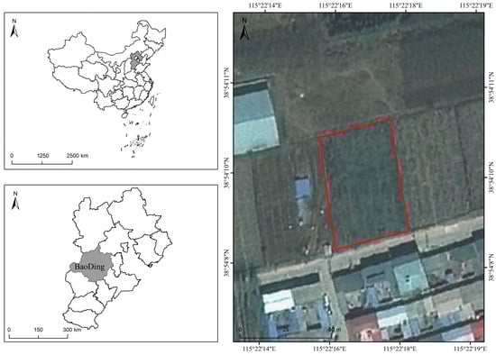
Figure 2.
Overview of the study area. The figure presents the geographical location of the study area, with the specific boundaries highlighted by a red box, and provides information on the country, province, and relevant background of the region.
2.2. Data Acquisition and Processing
2.2.1. Leaf Sample Collection
Leaf samples used in this study were collected from April to July 2025, covering two phenological stages of the apple trees: the bloom and fruit-set stage and the fruit-enlargement stage. The bloom and fruit-set stage is a critical phase of reproductive growth in apple trees, during which nitrogen, as a fundamental component of cellular structure and bioactive compounds, provides the necessary nutritional support for flowering and fruit-set. During the fruit-enlargement stage, fruit growth is mainly driven by cell division and expansion; nitrogen contributes to the synthesis of biological macromolecules such as proteins and nucleic acids, thereby supporting these processes.
Leaf sampling was conducted at 15-day intervals, and a total of 1120 leaf samples were collected. For each sampled tree, leaves were taken from two vertical positions (the upper canopy and the lower canopy). At each position, leaves were randomly selected in the horizontal direction by sampling four leaves at 90° intervals in a clockwise order. All sampled leaves were healthy and undamaged. After collection, surface dust and debris were gently removed using distilled water, and the leaves were air-dried and sealed in labeled bags for subsequent hyperspectral measurements.
2.2.2. Acquisition of Leaf Hyperspectral Reflectance Curves
The hyperspectral reflectance curves of the collected leaf samples were measured using an Optpsky ATP2400 spectrometer (Aopu Tiancheng Photoelectric Co., Ltd., Xiamen, China). The instrument has a spectral resolution of 0.5 nm and is capable of acquiring spectral information across the wavelength range of 180–1100 nm. To ensure consistency in spectral acquisition and to minimize the influence of unstable illumination and stray light, all measurements were conducted in a custom-built optical black box. An ATG1002 tungsten-halogen lamp (Aopu Tiancheng Photoelectric Co., Ltd., Xiamen, China) was used to simulate natural illumination conditions. Under sufficient and stable light intensity, the spectrometer integration time was set to 5000 ms. A calibrated reflectance reference panel was used for reflectance calibration. The probe was fixed to the optical measurement platform at a distance of 15 mm from the reference panel. After calibration, the probe position was kept unchanged, and each leaf sample was placed directly below the probe for measurement. For each leaf sample, four measurement points were recorded: the left side of the main vein, the right side of the main vein, the tip of the leaf, and the basal region near the petiole. The mean hyperspectral reflectance curve across the four measurement points was calculated and used as the final hyperspectral reflectance data for that leaf sample.
2.2.3. Leaf Nitrogen Content Analysis
After acquiring the hyperspectral reflectance data, LNC was determined using the Kjeldahl method, as expressed in Equation (1) [18]. Each leaf sample was first cut to an appropriate size and oven-dried to a constant weight. The dried material was then ground into a fine powder and sieved through a 0.45 mm mesh sieve. The sieved powder was digested with concentrated sulfuric acid and a catalyst, with a small amount of hydrogen peroxide was added dropwise as needed to facilitate digestion. The digested solution was subsequently processed and analyzed using a KDN-812 Kjeldahl nitrogen analyzer (Shanghai HuYueMing Scientific Instrument Co., Ltd., Shanghai, China).
A descriptive statistical analysis was conducted on the measured LNC. During the bloom and fruit-set stage, LNC ranged from approximately 2.02% to 3.34%. During the fruit-enlargement stage, LNC ranged from 1.62% to 2.68%. These differences are likely attributable to physiological variations across phenological stages in the annual growth cycle and to the fertilization management strategy of the orchard. A detailed statistical summary is provided in Table 1.

Table 1.
Statistical results of nitrogen content in apple leaf samples.
2.3. Spectral Data Processing and Characteristic Wavelength Extraction
2.3.1. Preprocessing of Hyperspectral Reflectance Curves
Preprocessing of hyperspectral reflectance curves was conducted to reduce acquisition-related interference, suppress irrelevant spectral variations, and establish a reliable data basis for subsequent feature extraction and modeling. In this study, the hyperspectral reflectance data of the leaf samples were preprocessed using multiplicative scatter correction (MSC) and Savitzky–Golay (SG) filtering. MSC was applied to mitigate the influence of spectral scattering, thereby minimizing undesired spectral variability among samples and enhancing the accuracy of the spectral information [19]. SG filtering was subsequently applied to smooth the spectra by locally fitting a polynomial, which suppressed high-frequency noise while preserving the overall trend of the original signal [20].
2.3.2. Characteristic Wavelength Selection for LNC
Hyperspectral spectroscopy provides continuous, high-resolution spectral measurements of the sample, and the resulting hyperspectral reflectance spectra contain highly abundant spectral information.
CARS is an iterative variable selection method inspired by the principle of “survival of the fittest”. It uses repeated Monte Carlo sampling to fit partial least squares (PLS) regression models at each iteration, and progressively eliminates uninformative wavelength variables probabilistically via adaptive reweighted sampling and an exponential decay function [21].
SPA is a forward feature selection method designed to address multicollinearity in high-dimensional spectral data. The algorithm evaluates collinearity among variables through projection operations and progressively selects combinations of wavelengths that carry maximal information while minimizing redundancy [22]. Therefore, this study employed a combination of CARS and SPA to select characteristic wavelengths from the preprocessed hyperspectral reflectance curves of the leaf samples.
2.4. Model Construction and Evaluation
2.4.1. Machine Learning Algorithms
In this study, regression models for apple LNC were established based on four machine learning algorithms: SVR, RF, XGBoost, and back-propagation neural network (BPNN).
SVR constructs an optimal predictive hyperplane in a high-dimensional feature space such that the sum of distances from the data points to this hyperplane is minimized. Owing to the flexibility of its kernel functions, SVR exhibits strong generalization ability when working with limited sample sizes and high-dimensional features [23].
RF is an ensemble learning method based on decision trees. It trains multiple decision trees on bootstrap-resampled subsets of the data and averages their outputs to generate the final prediction. At each split, a random subset of features is considered to determine the splitting rule, which makes RF suitable for large-scale nonlinear data [24].
XGBoost is an optimized implementation of the Gradient Boosting Decision Trees (GBDT). It uses a second-order Taylor expansion of the loss function, incorporates explicit regularization, and updates tree depth and leaf weights after each iteration. These features make XGBoost a fast, scalable, and regularized tree boosting method [25].
BPNN is based on a multilayer perceptron enhanced with a backpropagation algorithm. It minimizes prediction error by calculating gradients to adjust the connection weights. This error is propagated backward from the output layer to the input layer to optimize the network, thereby improving its capacity to fit nonlinear data [26].
The dataset was constructed by using the selected characteristic wavelengths as predictor variables and the LNC determined by the Kjeldahl method as the target variable. The data were split in a 7:2:1 ratio into a training set ( = 392), a validation set ( = 112), and a test set ( = 56). Model development and evaluation were implemented on a Windows 10 system using Python 3.12 and MATLAB 2018.
2.4.2. Model Evaluation Metrics
To assess the predictive performance of the regression models, two evaluation metrics were employed:
(1) The coefficient of determination () quantifies the proportion of variance in the observed response explained by the model; values closer to 1 indicate a better fit to the data [27]. The calculation is given in Equation (1).
where is the number of samples in the dataset, is the measured value of the -th sample, is the predicted value of the -th sample, and is the mean of the measured values for all samples in the dataset.
(2) The root mean squared error () measures the average magnitude of the deviation between predicted and observed values; smaller values indicate lower prediction error and thus better predictive performance [28]. The calculation is given in Equation (2).
where is the number of samples in the dataset, is the measured value of the -th sample, and is the predicted value of the -th sample.
To further determine whether there is a statistically significant difference in the prediction accuracy of the models on the test set samples, the Wilcoxon signed-rank test was employed for significance testing. The squared error was adopted as the error metric, as shown in Equation (3).
where denotes the squared error of mdel on the -th sample, is the measured value of the -th sample, and is the predicted value of the -th sample from model.
To further control the Family-Wise Error Rate, the Holm–Bonferroni correction was applied to the multiple tests. A result was deemed statistically significant if the adjusted p-value was less than 0.05.
2.5. Model Hyperparameter Optimization
2.5.1. Swarm-Based Optimization Algorithms
For hyperparameter optimization, this study used three swarm-based optimization algorithms as the baseline optimization strategies: PSO, crested porcupine optimizer (CPO) and black-winged kite algorithm (BKA). For each algorithm, both the population initialization stage and the iterative search process were improved.
PSO simulates flocking and foraging behavior in birds, where the population cooperatively searches for an optimal solution. Each particle represents a candidate solution and iteratively updates its position and velocity to approach the optimum, and PSO is characterized by a simple parameter structure and ease of implementation [29].
CPO is inspired by the defensive behavior of crested porcupines and models four protective mechanisms: visual warning, acoustic signaling, odor emission, and physical attack. In contrast to algorithms that primarily simulate offensive behavior, CPO emphasizes defensive strategies, improving adaptability to diverse threats and maintaining population diversity [30].
BKA is inspired by the hunting and migratory behavior of black-winged kites. Its hunting phase integrates global exploration and local exploitation, enhancing the balance between search breadth and depth. During migration, dynamic leader selection and leader adjustment steer the population toward the current best solution, yielding fast search speed and high convergence efficiency [31].
2.5.2. Improvements to Swarm-Based Optimization Algorithms
In swarm-based optimization algorithms, the population initialization phase is a critical first step that significantly influences the effectiveness of subsequent exploration and exploitation. Therefore, this study proposed an improved initialization strategy. The Sobol sequence was introduced to replace purely random population initialization, so that the initial individuals in the population are distributed more uniformly and efficiently in the solution space.
The Sobol sequence is a commonly used low-discrepancy sequence in Quasi Monte Carlo (QMC) methods. By minimizing discrepancy in the distribution of sampled points, it generates point sets with superior space-filling properties, making it widely applicable in numerical integration, optimization, and simulation problems. The Sobol sequence defines the initial direction numbers for the -th dimension, as shown in Equation (4), and these initial direction numbers are required to be odd and must satisfy for .
where denotes the bitwise exclusive OR operation in binary arithmetic.
Each initial direction numerator is converted to a direction number , which is used to construct a fixed binary fraction for the sequence coordinates. This conversion is defined in Equation (5).
Furthermore, the coordinate of the -th point in the -th dimension is given in Equation (6) [32].
where represents the -th significant bit in the binary representation of the index , and denotes the bitwise exclusive OR operation in binary arithmetic.
In addition, EOBL was integrated into both the population initialization phase and the iterative search process. EOBL extends the concept of opposition-based learning by introducing the notion of elite individuals. Individuals with high fitness in the current population are selected, and their opposite solutions are computed, as defined in Equation (7) [32]. For each pair, the superior solution between the current candidate and its opposite is retained as the offspring for the next generation. This strategy broadened exploration of the search space, enabling the algorithm to identify higher-quality solutions across a broader region, enhancing population diversity, and accelerating convergence.
where denotes the -th individual in the -th dimension, the parameters and represent the lower and upper bounds of the -th dimension, respectively.
Three improved optimization algorithms were obtained in this study, namely SEO-PSO, SEO-CPO, and SEO-BKA, and their performance was comparatively analyzed using the CEC2017 benchmark function set. CEC2017 comprises 29 test functions (F1–F29), categorized into four types: unimodal functions (F1–F2), simple multimodal functions (F3–F9), hybrid functions (F10–F19), and composition functions (F20–F29). The benchmark also supports multiple choices of problem dimensions.
In this study, the dimension was set to ten (D = 10). For all algorithms, the population size was uniformly set to 256 individuals, the MaxFES = 100,000, and the algorithms were independently executed 51 times. The proportion of elite individuals was set to 50%. The reported fitness values and standard deviations were calculated as the mean results over the 51 independent runs.
3. Results
3.1. Description of Spectral Characteristic Curves
Preprocessed leaf hyperspectral reflectance curves were analyzed. Figure 3 presents the mean spectra measured during the bloom and fruit-set stage and the fruit-enlargement stage. The two stages exhibit broadly similar overall profiles, with discernible differences in reflectance within specific spectral regions.
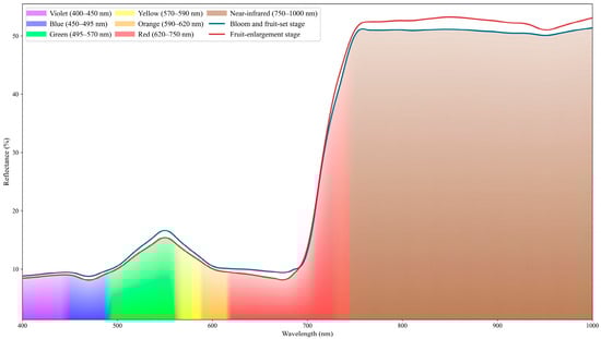
Figure 3.
Hyperspectral reflectance curves of leaf samples. The Figure compares hyperspectral reflectance curves of leaves from two phenological stages (bloom and fruit-set stage, fruit-enlargement stage), showing spectral bands (400–1000 nm) and reflectance values (%), with different colors distinguishing band attributes. Please refer to the abbreviation table for the abbreviations in the figure.
In the visible spectral region, leaf reflectance is relatively low. In the 450–490 nm range, chlorophyll a and chlorophyll b absorb blue light intensely, forming an absorption trough near 470 nm. During the early phenological stage (bloom and fruit set stage), chlorophyll concentration in the leaves is relatively low, resulting in higher reflectance in this stage. A reflectance peak occurs near 550 nm because chlorophyll exhibits weaker absorption in the green spectral region, so a greater portion of green light is reflected. As development proceeds, chlorophyll content in the leaves increases and the foliage darkens. A pronounced absorption trough forms in the red spectral band near 670 nm. Beyond the red band, as the spectrum enters the red-edge band, reflectance rises sharply near 680 nm. When chlorophyll content is high, the red-edge slope becomes steeper and the inflection point shifts toward longer wavelengths; this phenomenon is termed the red-edge shift. At longer wavelengths, reflectance stabilizes over roughly 750–1000 nm. The high reflectance in this region is largely governed by internal leaf structure, as cell walls and intercellular air spaces in the mesophyll strongly scatter near-infrared (NIR) radiation. As leaves develop and mature, NIR reflectance generally increases. A weak absorption trough occurs near 970 nm, attributable to absorption by liquid water within the leaf. In the study region, July marks the onset of the rainy season, which explains the more pronounced water absorption feature compared to early spring.
3.2. Characteristic Wavelength Selection Results
Characteristic wavelengths for LNC were selected and analyzed using the CARS–SPA method. The results for the bloom and fruit-set stage and for the fruit-enlargement stage are shown in Figure 4 and Figure 5, respectively.
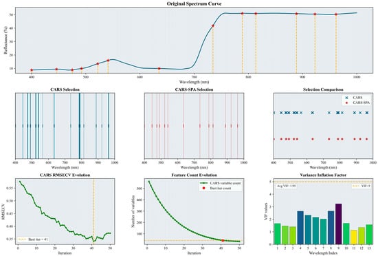
Figure 4.
Selected characteristic wavelengths for the bloom and fruit-set stage. The figure illustrates the results of the characteristic spectral band extraction process. It includes specific characteristic wavelengths marked on the original spectral curve (indicated by red asterisks), a comparison of the number and positions of wavelengths selected by CARS and CARS-SPA using lines of two different colors, the RMSECV history curve from the CARS iterations (with the optimal number of iterations and corresponding result marked by a yellow dashed line), and a histogram of the VIF values for the characteristic wavelengths. Please refer to the abbreviation table for the abbreviations in the figure.
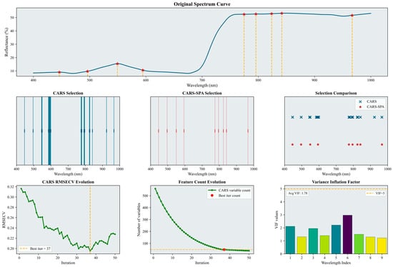
Figure 5.
Selected characteristic wavelengths for the fruit-enlargement stage. The figure illustrates the results of the characteristic spectral band extraction process. It includes specific characteristic wavelengths marked on the original spectral curve (indicated by red asterisks), a comparison of the number and positions of wavelengths selected by CARS and CARS-SPA using lines of two different colors, the RMSECV history curve from the CARS iterations (with the optimal number of iterations and corresponding result marked by a yellow dashed line), and a histogram of the VIF values for the characteristic wavelengths. Please refer to the abbreviation table for the abbreviations in the figure.
As shown in Figure 4, the initial CARS screening selected 40 wavelengths (6.7% of the full wavelength set). The subsequent CARS–SPA screening reduced this to 13 wavelengths (2.2%). These selected characteristic wavelengths were predominantly located within the 400–650 nm range. Based on the variance inflation factor results (average VIF = 1.95), collinearity among the selected wavelengths was effectively controlled.
As shown in Figure 5, the initial CARS screening selected 48 wavelengths (7.8% of the full set). The subsequent CARS–SPA screening reduced this to 9 wavelengths (1.5%). The selected characteristic wavelengths were distributed relatively evenly across two spectral regions: 400–650 nm and 800–1000 nm. The variance inflation factor results (average VIF = 1.78) indicate that collinearity among the selected wavelengths was effectively controlled.
A comparison of the two phenological stages reveals that the characteristic wavelengths are predominantly within the visible region, suggesting these bands carry substantial information on LNC. Furthermore, these wavelengths demonstrate sensitivity to leaf physiological status and relatively stable spectral responses across both stages, thereby effectively representing the core spectral characteristics of leaves.
3.3. Performance Evaluation of Optimization Algorithms
3.3.1. Benchmarking Results for the Original Optimization Algorithms
The performance of the optimization algorithms was evaluated using the CEC2017 benchmark function set. Figure 6 presents the mean fitness values and the standard deviations across iterations for PSO, CPO, and BKA. A logarithmic axis was adopted in the plots to avoid compressing results with small magnitudes due to the large differences in numerical scale among the test functions.
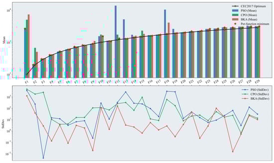
Figure 6.
Performance test results of the original swarm-based optimization algorithms. The figure presents two plots on a logarithmic scale: a bar chart displaying the mean results across test functions, where the height of the bars indicates the effectiveness of the optimization algorithms (with the optimal algorithm marked), and a line chart showing the StdDev results, which illustrates the stability of the algorithm’s performance based on the degree of fluctuation. Please refer to the list of abbreviations for the acronyms used in the figure.
Overall, BKA exhibited the most robust performance among the three algorithms in this benchmark. It achieved the best mean fitness in 12 out of the 29 test functions, with a relatively small standard deviation across iterations, indicating greater stability throughout the optimization process. In the unimodal functions (F1–F2), PSO attatined superior fitness values. The simple structure of the Unimodal test functions, characterized by a single global optimum and absence of local optima, allows PSO to leverage its inherent capacity for rapid convergence effectively. In the simple multimodal functions (F3–F9), differences in mean fitness among the three algorithms narrowed markedly. Although PSO retains a slight advantage, the introduction of multiple local optima complicates the search landscape, and in this context, the specialized iterative strategies of CPO and BKA adapt better to this structure. In terms of the standard deviations across iterations, BKA exhibits more stable search behavior than PSO and CPO. In the hybrid functions (F10–F19), BKA achieved the best fitness. Hybrid functions partition the search space into subspaces defined by different base functions; consequently, the same function can exhibit markedly different landscape characteristics across regions, increasing optimization difficulty and complexity. PSO is prone to premature convergence or stagnation in specific subspaces, thereby exhibiting limited effectiveness in such mixed and complex environments. In the composition functions (F20–F29), BKA continued to perform strongly; however, CPO attained mean fitness comparable to that of BKA alongside a more stable standard deviation across iterations.
Taken together, for relatively simple search landscapes, PSO demonstrates rapid global search. As landscape complexity increases, CPO and BKA yield superior results owing to their multi-level, interactive iterative strategies. The ability to attain the best fitness is, in part, determined by algorithmic design: more sophisticated update mechanisms better avoid entrapment in local optima and are therefore better suited to complex, high-dimensional search spaces. Additionally, across independent runs, random population initialization can affect algorithmic stability. An initial population distributed in low-quality regions can lead to slow early convergence. Accordingly, the initialization stage was improved in this study to mitigate this sensitivity and enhance stability.
3.3.2. Benchmarking Results for the Improved Optimization Algorithms
In this study, the optimization algorithms were improved by incorporating the Sobol sequence and EOBL. The results on the CEC2017 test function set are shown in Figure 7, which displays the mean fitness and the standard deviations across iterations for the three improved algorithms, SEO-PSO, SEO-CPO, and SEO-BKA.
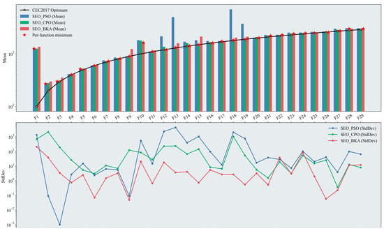
Figure 7.
Performance test results of the improved swarm-based optimization algorithms. The figure presents two plots on a logarithmic scale: a bar chart displaying the mean results across test functions, where the height of the bars indicates the effectiveness of the optimization algorithms (with the optimal algorithm marked), and a line chart showing the StdDev results, which illustrates the stability of the algorithm’s performance based on the degree of fluctuation. Please refer to the list of abbreviations for the acronyms used in the figure.
Overall, SEO-BKA achieved the best mean fitness for 14 out of 29 test functions. Its standard deviation across iterations was lower than that of BKA, indicating more stable search behavior. These results collectively validate the effectiveness of the proposed improvements in both the initialization and iterative search phases. In the unimodal functions (F1–F2), SEO-PSO continued to perform well. Relative to the baseline algorithms, differences in mean fitness among the three improved variants narrowed further, with meant closer to the functions’ optimal fitness values. The incorporation of the EOBL mechanism during iterations enhanced the convergence speed and precision of both CPO and BKA on such simple landscapes. In the simple multimodal functions (F3–F9), the three improved algorithms performed comparably, with SEO-CPO slightly outperforming the others. The improvements yielded more uniform population initialization and higher-quality initial candidates, enhancing the global exploration capability of CPO and BKA. In terms of the standard deviation across iterations, SEO-BKA remained stable under the modifications and stayed within a favorable range, indicating consistent run-to-run convergence around a stable fitness level. In the hybrid functions (F10–F19), SEO-CPO attained the lowest mean fitness on 6 of the 10 functions, while SEO-BKA achieved the best values on the remaining 4; by contrast, SEO-PSO was no longer competitive in this category. This pattern indicates that, although the improvement strategy enhances performance to some extent, the intrinsic structural characteristics of each algorithm remain the primary determinant when tackling complex, high-dimensional problems. In the composition functions (F20–F29), the performance of SEO-BKA was largely comparable to that of BKA. However, on these more challenging functions, SEO-BKA achieved the best mean fitness in 8 out of 10 cases. Moreover, its standard deviation across iterations remained within a consistently stable range from the hybrid to the composition function groups, indicating robust convergence behavior.
Figure 8a,b present the mean runtime per run for each optimization algorithm. As test-function complexity increases, average runtime rises accordingly. For the unimodal (F1–F2) and simple multimodal (F3–F9) functions, runtimes remain within 10 s. Runtimes increase for the hybrid functions (F10–F19) and reach a maximum of 42 s for the composition functions (F20–F29). PSO demonstrated relatively fast execution on F1-F2 and F3–F9, but exhibited a pronounced slowdown on the F10–F19 and F20–F29 compared to CPO and BKA. Across the benchmark, BKA recorded the second-fastest mean runtime, whereas CPO was the slowest. With the improvements, all three algorithms run faster: on the unimodal (F1–F2), simple multimodal (F3–F9), and hybrid (F10–F19) groups, mean runtime decreases by 2–5 s; on the composition functions (F20–F29), it decreases by 10–15 s. Notably, SEO-BKA reduces runtime by 36.7% relative to BKA.
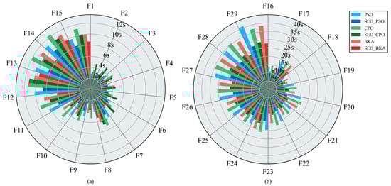
Figure 8.
Average runtime per run for the optimization algorithms: (a) results for test functions F1–F15; (b) results for test functions F16–F29. The figure shows the single test running time of swarm optimization algorithms in subfigures (a,b). Different colors represent different algorithms, and bar lengths indicate the computation time. Please refer to the abbreviation table for the abbreviations in the figure.
Overall, SEO-BKA delivered the best performance across the benchmark. The inherent hunting and migration behaviors in BKA facilitate a balance between global exploration and local exploitation. The incorporated Cauchy mutation strategy aids in escaping local optima, thereby strengthening global search capabilities. With the proposed improvements, the Sobol sequence and EOBL produce a more uniform population at initialization, yielding higher-quality initial candidates, as shown in Figure 9a–c. Additionally, integrating EOBL with a leader strategy enhances leader selection during the migration phase while preserving population diversity.
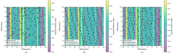
Figure 9.
Results of improved BKA population initialization: (a) random initialization; (b) Sobol initialization; (c) SEO initialization. The figure illustrates the population initialization of the improved BKA algorithm in subfigures (a–c), showing fitness values represented by different color regions; elite individuals marked in red to illustrate their distribution within the initial population; and the population coverage across the search space. Please refer to the abbreviation table for the abbreviations in the figure.
3.4. Model Development and Evaluation Results
3.4.1. Results for the Bloom and Fruit-Set Stage
In this study, characteristic hyperspectral reflectance data acquired during the bloom and fruit-set stage were used, and hyperparameters were optimized by means of optimization algorithms. Four machine learning regression models were then developed to invert LNC. The evaluation metrics of these models are summarized in Table 2.
Table 2.
Model evaluation metrics with swarm-based optimization algorithms for the bloom and fruit-set stage.
According to the evaluation metrics, the RF and XGBoost models performed well overall, with test-set values predominantly in the 0.83–0.85 range. BPNN performed slightly worse, whereas SVR yielded lower values (maximum = 0.795). The tree-based ensemble methods outperformed the kernel-based approach in modeling complex nonlinear relationships within the data, even when SVR employed an RBF kernel with strong nonlinear capacity. For BPNN, a sufficiently large dataset is required to train and define the network architecture, and the model is highly sensitive to hyperparameter settings; consequently, its performance was less stable than that of the tree-based models. Among the optimization algorithms pairs, BKA–XGBoost achieved the best performance ( = 0.859, = 0.128). Figure 10 shows the error distributions of the models. BKA–RF yielded comparable results ( = 0.852, = 0.127), and CPO delivered relatively strong performance for the SVR and BPNN models.

Figure 10.
Results of the BKA-XGBoost model: (a) inversion line chart; (b) error distribution histogram. The figure shows the prediction results of the BKA-XGBoost model. In the line chart, different colors distinguish the actual values and predicted values. The error distribution histogram displays the prediction error values and their corresponding frequencies. Please refer to the abbreviation table for the abbreviations in the figure.
Table 3 presents the evaluation metrics of the regression models after hyperparameter tuning using the improved optimization strategies. Overall, model performance improved following the integration of the proposed enhancement strategies. RF and XGBoost continued to deliver strong regression performance, with values exceeding 0.85 on both the validation and test sets. The of the SEO-CPO-SVR model increased from 0.795 to 0.811. The SEO-BKA-BPNN model ( = 0.870, = 0.130) outperformed the original CPO-BPNN model ( = 0.829, = 0.140). SEO-BKA-XGBoost achieved the best overall performance ( = 0.883, = 0.124). Figure 11 shows the error distributions of the models. Hyperparameter optimization yielded more pronounced gains for XGBoost than for RF; SEO–BKA–RF attains = 0.877 and = 0.127. In several models, the increase in validation-set exceeded that in the test set, suggesting that the hyperparameters were configured more effectively during model development, while the concurrent improvements on the test set indicate enhanced generalization capability. Overall, these results show that incorporating the improved optimization algorithms has a positive impact on hyperparameter optimization for the machine learning models.
Table 3.
Model evaluation metrics with improved swarm-based optimization algorithms for the bloom and fruit-set stage.
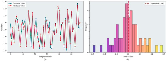
Figure 11.
Results of the SEO-BKA-XGBoost model: (a) inversion line chart; (b) error distribution histogram. The figure shows the prediction results of the SEO-BKA–XGBoost model. In the line chart, different colors distinguish the actual values and predicted values. The error distribution histogram displays the prediction error values and their corresponding frequencies. Please refer to the abbreviation table for the abbreviations in the figure.
Based on the comparative results of prediction performance, the top-performing SEO-BKA-XGBoost was selected as the benchmark model. Under identical optimization conditions, significance testing was conducted against the other models, with the results presented in Table 4.
Table 4.
Statistical significance of improved swarm-based models for bloom and fruit-set stage.
The Mean Error values were consistently negative, indicating that SEO-BKA-XGBoost produced smaller sample-wise errors than the other models and exhibited more stable predictive performance. In terms of significance level, the largest performance gap was observed between SEO-BKA-XGBoost and SEO-BKA-SVR, with an adjusted p-value of 5.20 × 10⁻⁵, demonstrating strong statistical significance. The other two comparisons showed relatively weaker, yet still significant, differences. These results further show that tree-based ensemble methods tend to be more robust and stable when modeling complex nonlinear relationships.
3.4.2. Results for the Fruit-Enlargement Stage
In this study, characteristic hyperspectral reflectance data acquired during the fruit-enlargement stage were used, and hyperparameters were optimized by means of optimization algorithms. Four machine learning regression models were then developed to invert LNC. The evaluation metrics of these models are summarized in Table 5.
Table 5.
Model evaluation metrics with swarm-based optimization algorithms for the fruit-enlargement stage.
Based on the evaluation metrics, inversion accuracy during the fruit-enlargement stage exceeded that of the bloom and fruit-set stage. Overall, RF and XGBoost continued to perform well, and SVR and BPNN also showed improved accuracy. From the perspective of optimization algorithm, BKA remained the most effective. BKA–RF and BKA–XGBoost performed similarly on the test set; the slightly lower RMSE identified BKA–RF as the best model ( = 0.874, = 0.084). Figure 12 shows the error distributions of the models.
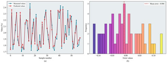
Figure 12.
Results of the BKA-XGBoost model: (a) inversion line chart; (b) error distribution histogram. The figure shows the prediction results of the BKA–XGBoost model. In the line chart, different colors distinguish the actual values and predicted values. The error distribution histogram displays the prediction error values and their corresponding frequencies. Please refer to the abbreviation table for the abbreviations in the figure.
With the introduction of the improved optimization algorithms, the predictive accuracy of all models increased. The results are summarized in Table 6. Notably, XGBoost achieved values exceeding 0.86, and SEO–BKA–XGBoost delivered the best performance ( = 0.897, = 0.069). Figure 13 shows the error distributions of the models. The maximum prediction values for SEO–BKA–SVR and SEO–CPO–BPNN reach 0.816 and 0.850, respectively. By comparison, SEO–BKA–RF showed a smaller improvement ( = 0.876, = 0.080). The evaluation metrics likewise confirm that the models’ nonlinear fitting capability remains effective during the fruit-enlargement stage.
Table 6.
Model evaluation metrics with improved swarm-based optimization algorithms for the fruit-enlargement stage.
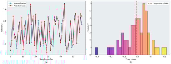
Figure 13.
Results of the SEO-BKA-XGBoost model: (a) inversion line chart; (b) error distribution histogram. The figure shows the prediction results of the SEO-BKA–XGBoost model. In the line chart, different colors distinguish the actual values and predicted values. The error distribution histogram displays the prediction error values and their corresponding frequencies. Please refer to the abbreviation table for the abbreviations in the figure.
Similarly, significance testing was conducted for the models in the fruit swelling stage, again using SEO-BKA-XGBoost as the benchmark. The results are presented in Table 7.
Table 7.
Statistical significance of improved swarm-based models for the fruit-enlargement stage.
The Mean Error values remained negative, consistent with the results from the bloom and fruit-set stage. However, a notable variation was observed in the Mean Error relative to SEO-BKA-BPNN, indicating that the error distribution of BPNN lacks stability and that the disparity with XGBoost widened within specific intervals. Overall, the superior performance of the SEO-BKA-XGBoost model is not coincidental; it not only excelled in overall metrics such as R2 and RMSE but also exhibited a consistently lower trend at the sample error level.
4. Discussion
In this study, the Sobol sequence and EOBL were incorporated into three swarm-based optimization algorithms (PSO, CPO, and BKA), yielding three improved algorithm variants: SEO-PSO, SEO-CPO, and SEO-BKA. Random population initialization is a common approach. Although this approach is simple to implement and preserves a certain degree of exploratory ability, low-quality individuals offer limited guidance for directing the population toward high-quality solutions and may even impair the overall optimization efficiency [33]. For this reason, improving the population initialization stage has become a major focus in many studies [34,35]. Although diverse strategies have been proposed, they share the aim of producing a more uniform, space-filling initial population that achieves better coverage of the search space. QMC methods perform numerical integration by replacing pseudorandom samples with deterministic low-discrepancy sequences. The Sobol sequence used in this study is a widely used low-discrepancy sequence within the QMC family. Jun Zhu (2012) [36] compared the performance of the Sobol sequence with other QMC methods, including the Halton sequence and lattice rules, and reported that the Sobol sequence offers higher computational efficiency for low-dimensional problems. In particular, when the initial direction numbers and primitive polynomials are optimized, it can attain rapid convergence with fewer sample points. However, the study also noted that in high-dimensional settings, the efficacy of QMC methods degrades due to increasing dimension-dependent discrepancy, and optimization procedures initialized with such sequences can stagnate in local optima.
To address this issue, EOBL employs an opposition-based update to feedback information from elite solutions into the search process, thereby accelerating the identification of superior candidates and mitigating premature convergence to local optima [37]. In this study, EOBL was integrated with the Sobol sequence to mitigate its limitations in high-dimensional settings. By computing the opposite solution of the current elite and retaining the superior candidate, the search can escape local-optimum regions around the elite and explore more promising regions of the search space, which contributes to an accelerated convergence rate. Comparative experiments on the CEC2017 benchmark function set showed that the improved algorithm achieved clear advantages over the original algorithm in both convergence speed and best fitness, while also reducing the mean runtime. These results confirm the effectiveness of the proposed improvement strategy.
The enhanced performance of the optimizers was directly reflected in superior predictive accuracy of machine learning models, with consistent increases in and marked decreases in across all models. In this study, four machine learning regression models, namely SVR, RF, XGBoost, and BPNN, were constructed to invert LNC. Across both phenological stages, the SEO-BKA-XGBoost model demonstrated the best overall performance. This result is jointly determined by both the selected hyperparameter combination and the intrinsic structural characteristics of the algorithm. XGBoost constructs an ensemble of decision trees through a boosting strategy in which trees are trained sequentially so that each new tree focuses on fitting the residuals of the previous trees. Furthermore, XGBoost incorporates a second-order Taylor expansion and explicit regularization, which enhance fitting precision while mitigating the risk of overfitting [38]. In contrast, RF constructs multiple decision trees through bagging and random feature selection. The individual trees are trained independently and in parallel, and prediction is obtained by simple averaging or voting [39]. Hamid Jafarzadeh et al. (2021) reported that, for hyperspectral data, XGBoost outperformed RF [40]. Xibin Dong et al. (2020) conducted a systematic comparison of bagging and boosting, concluding that bagging exhibits greater robustness to noise, while boosting tends to achieve superior performance under low-noise conditions with large training sets [41]. In this study’s experimental results, the performance of the RF model was competitive with, yet slightly inferior to, that of XGBoost—a finding that aligns with the aforementioned studies.
In this study, characteristic wavelengths were selected from the hyperspectral reflectance data using the CARS-SPA algorithm. Although the selection is driven primarily by statistical regression relationships, the resulting characteristic wavelengths encode rich physiological and biochemical information about the leaves. Within the CARS-SPA pipeline, CARS served as the preliminary filter by directly evaluating correlations between full-spectrum reflectance and LNC, whereas SPA was employed to reduce multicollinearity among the selected wavelengths. The results demonstrate that recurrent characteristic wavelengths were identified across both phenological stages, distributed across both the visible (400–700 nm) and near-infrared (NIR, 700–1000 nm) regions. Notable examples include 450, 480, 541, 780, and 975 nm. These characteristic wavelengths carry substantial information about LNC. Anran Qin et al. (2025) [42] used SPA to identify sensitive wavelengths for apple trees at the spring shoot stop-growing stage (NSS) and the autumn shoot stop-growing stage (ASS). The sensitive wavelengths were primarily centered around 420, 550, 730, and 997 nm, which is broadly consistent with the characteristic wavelengths identified in the present study. Chuanqi Xie et al. (2018) systematically evaluated the feasibility of assessing maize nitrogen status using spectral reflectance and reported that nitrogen-sensitive wavelengths were concentrated in the 350–1000 nm range, with 555 and 730 nm as representative wavelengths [43].
With respect to sample diversity, this study focused on two phenological stages, the bloom and fruit-set stage and the fruit-enlargement stage. However, the nitrogen dynamics of fruit trees across the annual growth cycle form a continuous process. Leaves at different phenological stages exhibit distinct physiological and metabolic traits, which in turn lead to differences in their spectral response mechanisms. Therefore, discrepancies in model-derived estimates across different measurement periods may not necessarily indicate model instability; rather, they are likely the combined consequence of phenology-driven physiological variation and differences in acquisition conditions. In the present study, the baseline of leaf nitrogen content (LNC) varied between stages: during the bloom and fruit-set stage, LNC ranged from 2.02% to 3.34%, whereas it declined to 1.62–2.68% during the fruit-enlargement stage. Such baseline shifts can lead to stage-dependent changes in the sensitivity of the same spectral bands to LNC, resulting in a phenology-specific response offset. Moreover, acquisition conditions are difficult to fully standardize across phenological stages. Although we minimized illumination-related effects by using a controlled optical setup and reflectance calibration, practical orchard deployment will inevitably encounter variations in illumination intensity and solar angle, canopy shading, and related field factors. To ensure that the proposed technique remains interpretable and operational in field applications, future work should adopt a phenology-aware and campaign-consistent deployment strategy. From a decision-making perspective, predictions should be interpreted against stage-specific reference ranges rather than a single global threshold. From an operational perspective, standardized acquisition protocols should be implemented, including a fixed time-of-day window, consistent sensor–leaf geometry, routine reflectance calibration, and a small number of destructive chemical measurements within each measurement period to correct potential inter-period bias.
In addition, this study examined a single cultivar (Mollies). Differences among apple cultivars in growing environment, physiological and metabolic characteristics, and leaf structural traits can lead to distinct spectral signatures even under equivalent leaf nitrogen level. Accordingly, future work should extend to additional cultivars—Fuji, Gala, and Golden Delicious—to elucidate the physiological and biochemical bases of cultivar-specific spectral signatures, thereby enhancing the generalizability and practical applicability of the hyperspectral inversion models.
Regarding sample size, 1120 leaf samples were collected in this study. Models trained on this dataset exhibited strong performance under single-cultivar, stage-specific conditions. However, larger-scale datasets can enable machine learning models to capture more complex nonlinear relationships. Future work should integrate multiple apple cultivars and phenological stages to construct a comprehensive dataset, thereby enhancing model generalizability and stability.
Regarding data acquisition, manual sampling was combined with laboratory measurements. Future work should explore in situ, non-destructive sensing. Because field illumination is highly variable, spectral correction methods that account for varying viewing geometries and illumination conditions are needed to improve the reliability of in-field model deployment.
5. Conclusions
Nitrogen is one of the key indicators for evaluating the nutritional status and growth health of fruit trees. The combination of spectral techniques and machine learning algorithms has emerged as a powerful tool for the rapid and non-destructive assessment of LNC. In this study, leaf samples were collected from apple trees during the bloom and fruit-set stage and the fruit-enlargement stage. For each sample, hyperspectral reflectance curves and LNC were measured. Sobol sequences and EOBL were introduced to improve the swarm-based optimization algorithms, which were subsequently applied to optimize the hyperparameters of the machine learning models. The resulting machine learning regression models were applied to estimate LNC. The main conclusions are as follows:
(a) The CARS-SPA method effectively identifies characteristic wavelengths associated with LNC from the hyperspectral reflectance curves. For both phenological stages, the selected characteristic wavelengths are mainly concentrated in the visible spectral region. This finding demonstrates that variation in LNC within the visible spectral region is linked to physiological and biochemical processes, and that the spectral response of nitrogen to these processes exhibits considerable stability across phenological stages.
(b) Incorporating the Sobol sequence and the EOBL strategy improved the swarm-based optimization algorithms and enhanced both search accuracy and convergence speed for PSO, CPO, and BKA. Among the improved algorithms, SEO-BKA achieved the best performance. In a set of 29 benchmark functions, SEO-BKA achieved the best mean fitness in 14 functions, and the mean runtime was reduced by 36.7%.
(c) A comparative analysis was conducted for four machine learning regression models: SVR, RF, XGBoost, and BPNN. The results show that RF and XGBoost achieved higher overall accuracy than SVR and BPNN. The SEO-BKA-XGBoost model achieved the highest inversion accuracy for LNC in both phenological stages. It obtained the highest coefficient of determination, with equal to 0.883 and 0.897, and the lowest root mean square error, with equal to 0.124 and 0.069.
Author Contributions
Conceptualization, R.X.; Methodology, R.X.; Formal Analysis, R.X.; Investigation, H.R.; Data Curation, H.R.; Writing—Original Draft Preparation, R.X.; Writing—Review & Editing, Y.G.; Visualization, H.R.; Supervision, Z.R.; Project Administration, Z.R.; Funding Acquisition, Z.R. All authors have read and agreed to the published version of the manuscript.
Funding
This research was supported by the Hebei Provincial Department of Science and Technology (22327203D).
Data Availability Statement
The data that support the findings of this study are available from the corresponding author upon reasonable request. The data are not publicly available due to privacy concerns. Interested researchers may contact the corresponding author at renzh68@163.com.
Acknowledgments
The authors are grateful for the financial support from the Hebei Provincial Department of Science and Technology (Grant number 22327203D).
Conflicts of Interest
The authors declare no conflicts of interest.
Abbreviations
The following abbreviations are used in this manuscript:
| BKA | Back-winged kite algorithm |
| BO | Byesian optimization |
| BPNN | Back propagation neural network |
| CARS | Competitive adaptive reweighted sampling |
| CPO | Crested porcupine optimizer |
| EOBL | Elite opposition-based learning |
| GA | Genetic algorithms |
| GBDT | Gradient boosting decision tree |
| GSWOA | Global search whale optimization algorithm |
| KELM | Kernel extreme learning machine |
| LNC | Leaf nitrogen content |
| PSO | Particle swarm optimization |
| QMC | Quasi Monte Carlo |
| Coefficient of determination | |
| RF | Random forest |
| Root mean squared error | |
| SA | Simulated annealing |
| SEO | Sobol-Elite opposition-based learning |
| SPA | Successive projection algorithm |
| SVR | Support vector regression |
References
- Tarancón, P.; Fernández-Serrano, P.; Besada, C. Consumer perception of situational appropriateness for fresh, dehydrated and fresh-cut fruits. Food Res. Int. 2021, 140, 110000. [Google Scholar] [CrossRef]
- Medda, S.; Fadda, A.; Mulas, M. Influence of Climate Change on Metabolism and Biological Characteristics in Perennial Woody Fruit Crops in the Mediterranean Environment. Horticulturae 2022, 8, 273. [Google Scholar] [CrossRef]
- Wen, B.; Gong, X.; Chen, X.; Tan, Q.; Li, L.; Wu, H. Transcriptome analysis reveals candidate genes involved in nitrogen deficiency stress in apples. J. Plant Physiol. 2022, 279, 153822. [Google Scholar] [CrossRef] [PubMed]
- Cui, M.; Zeng, L.; Qin, W.; Feng, J. Measures for reducing nitrate leaching in orchards: A review. Environ. Pollut. 2020, 263, 114553. [Google Scholar] [CrossRef] [PubMed]
- Zipori, I.; Erel, R.; Yermiyahu, U.; Ben-gal, A.; Dag, A. Sustainable management of olive orchard nutrition: A review. Agriculture 2020, 10, 11. [Google Scholar] [CrossRef]
- Muñoz-Huerta, R.F.; Guevara-Gonzalez, R.G.; Contreras-Medina, L.M.; Torres-Pacheco, I.; Prado-Olivarez, J.; Ocampo-Velazquez, R.V. A review of methods for sensing the nitrogen status in plants: Advantages, disadvantages and recent advances. Sensors 2013, 13, 10823–10843. [Google Scholar] [CrossRef]
- Subi, X.; Eziz, M.; Zhong, Q.; Li, X. Estimating the chromium concentration of farmland soils in an arid zone from hyperspectral reflectance by using partial least squares regression methods. Ecol. Indic. 2024, 161, 111987. [Google Scholar] [CrossRef]
- Noda, H.M.; Muraoka, H.; Nasahara, K.N. Plant ecophysiological processes in spectral profiles: Perspective from a deciduous broadleaf forest. J. Plant Res. 2021, 134, 737–751. [Google Scholar] [CrossRef]
- Jiang, X.; Zhen, J.; Miao, J.; Zhao, D.; Shen, Z.; Jiang, J.; Gao, C.; Wu, G.; Wang, J. Newly-developed three-band hyperspectral vegetation index for estimating leaf relative chlorophyll content of mangrove under different severities of pest and disease. Ecol. Indic. 2022, 140, 108978. [Google Scholar] [CrossRef]
- Canova, L.d.S.; Vallese, F.D.; Pistonesi, M.F.; de Araújo Gomes, A. An improved successive projections algorithm version to variable selection in multiple linear regression. Anal. Chim. Acta 2023, 1274, 341560. [Google Scholar] [CrossRef]
- Moghimi, A.; Tavakoli Darestani, A.; Mostofi, N.; Fathi, M.; Amani, M. Improving forest above-ground biomass estimation using genetic-based feature selection from Sentinel-1 and Sentinel-2 data (case study of the Noor forest area in Iran). Kuwait J. Sci. 2024, 51, 100159. [Google Scholar] [CrossRef]
- Li, W.; Zhu, X.; Yu, X.; Li, M.; Tang, X.; Zhang, J.; Xue, Y.; Zhang, C.; Jiang, Y. Inversion of Nitrogen Concentration in Apple Canopy Based on UAV Hyperspectral Images. Sensors 2022, 22, 3503. [Google Scholar] [CrossRef] [PubMed]
- Zhao, X.; Zhao, Z.; Zhao, F.; Liu, J.; Li, Z.; Wang, X.; Gao, Y. An Estimation of the Leaf Nitrogen Content of Apple Tree Canopies Based on Multispectral Unmanned Aerial Vehicle Imagery and Machine Learning Methods. Agronomy 2024, 14, 552. [Google Scholar] [CrossRef]
- Guo, Y.; Fu, Y.H.; Chen, S.; Hao, F.; Zhang, X.; de Beurs, K.; He, Y. Predicting grain yield of maize using a new multispectral-based canopy volumetric vegetation index. Ecol. Indic. 2024, 166, 112295. [Google Scholar] [CrossRef]
- Luo, W.; Li, W.; Liu, S.; Li, Q.; Huang, H.; Zhang, H. Measurement of four main catechins content in green tea based on visible and near-infrared spectroscopy using optimized machine learning algorithm. J. Food Compos. Anal. 2025, 138, 106990. [Google Scholar] [CrossRef]
- Qin, Z.; Yang, H.; Shu, Q.; Yu, J.; Yang, Z.; Ma, X.; Duan, D. Estimation of Dendrocalamus giganteus leaf area index by combining multi-source remote sensing data and machine learning optimization model. Front. Plant Sci. 2024, 15, 1505414. [Google Scholar] [CrossRef]
- Khandelwal, K.; Nanda, S.; Dalai, A.K. Machine learning modeling of supercritical water gasification for predictive hydrogen production from waste biomass. Biomass Bioenergy 2025, 197, 107816. [Google Scholar] [CrossRef]
- Mirabdulbaghi, M. Leaf nutrient status of some grafted-pear rootstocks influenced by different soil types. Span. J. Agric. Res. 2020, 18, e0903. [Google Scholar] [CrossRef]
- Wan, C.; Yue, R.; Li, Z.; Fan, K.; Chen, X.; Li, F. Prediction of Kiwifruit Sweetness with Vis/NIR Spectroscopy Based on Scatter Correction and Feature Selection Techniques. Appl. Sci. 2024, 14, 4145. [Google Scholar] [CrossRef]
- Cho, G.H.; Kim, Y.J.; Jeon, K.; Joo, H.J.; Kang, K.S. Accuracy Evaluation of Visible-Near Infrared Spectroscopy for Detecting Insect Damage in Acorns of Quercus acuta. Silvae Genet. 2024, 73, 99–109. [Google Scholar] [CrossRef]
- Yang, D.; Hu, J. A detection method of oil content for maize kernels based on CARS feature selection and deep sparse autoencoder feature extraction. Ind. Crops Prod. 2024, 222, 119464. [Google Scholar] [CrossRef]
- Liu, J.; Xie, J.; Meng, T.; Dong, H. Organic matter estimation of surface soil using successive projection algorithm. Agron. J. 2022, 114, 1944–1951. [Google Scholar] [CrossRef]
- Tian, S.; Guo, H.; Xu, W.; Zhu, X.; Wang, B.; Zeng, Q.; Mai, Y.; Huang, J.J. Remote sensing retrieval of inland water quality parameters using Sentinel-2 and multiple machine learning algorithms. Environ. Sci. Pollut. Res. 2023, 30, 18617–18630. [Google Scholar] [CrossRef] [PubMed]
- Ganaie, M.A.; Tanveer, M.; Suganthan, P.N.; Snasel, V. Oblique and rotation double random forest. Neural Netw. 2022, 153, 496–517. [Google Scholar] [CrossRef] [PubMed]
- Chen, T.; Guestrin, C. XGBoost: A scalable tree boosting system. In Proceedings of the ACM SIGKDD International Conference on Knowledge Discovery and Data Mining, San Francisco, CA, USA, 13–17 August 2016; pp. 785–794. [Google Scholar]
- Sarkar, C.; Gupta, D.; Gupta, U.; Hazarika, B.B. Leaf disease detection using machine learning and deep learning: Review and challenges. Appl. Soft Comput. 2023, 145, 110534. [Google Scholar] [CrossRef]
- Berggren, M. Coefficients of Determination Measured on the Same Scale as the Outcome: Alternatives to R2 That Use Standard Deviations Instead of Explained Variance. Psychol. Methods 2024. [Google Scholar] [CrossRef]
- Hodson, T.O. Root-mean-square error (RMSE) or mean absolute error (MAE): When to use them or not. Geosci. Model Dev. 2022, 15, 5481–5487. [Google Scholar] [CrossRef]
- Wan, C.; Yang, J.; Zhou, L.; Wang, S.; Peng, J.; Tan, Y. Fertilization Control System Research in Orchard Based on the PSO-BP-PID Control Algorithm. Machines 2022, 10, 982. [Google Scholar] [CrossRef]
- Abdel-Basset, M.; Mohamed, R.; Abouhawwash, M. Crested Porcupine Optimizer: A new nature-inspired metaheuristic. Knowl.-Based Syst. 2024, 284, 111257. [Google Scholar] [CrossRef]
- Wang, J.; Wang, W.C.; Hu, X.X.; Qiu, L.; Zang, H.F. Black-Winged Kite Algorithm: A Nature-Inspired Meta-Heuristic for Solving Benchmark Functions and Engineering Problems; Springer: Dordrecht, The Netherlands, 2024; Volume 57. [Google Scholar]
- Joe, S.; Kuo, F.Y. Remark on Algorithm 659: Implementing Sobol’s quasirandom sequence generator. ACM Trans. Math. Softw. 2003, 29, 49–57. [Google Scholar] [CrossRef]
- Pan, W.; Li, K.; Wang, M.; Wang, J.; Jiang, B. Adaptive randomness: A new population initialization method. Math. Probl. Eng. 2014, 2014, 975916. [Google Scholar] [CrossRef]
- Du, C.; Zhang, J.; Fang, J. An innovative complex-valued encoding black-winged kite algorithm for global optimization. Sci. Rep. 2025, 15, 932. [Google Scholar] [CrossRef] [PubMed]
- Zhang, Z.; Wang, X.; Yue, Y. Heuristic Optimization Algorithm of Black-Winged Kite Fused with Osprey and Its Engineering Application. Biomimetics 2024, 9, 595. [Google Scholar] [CrossRef] [PubMed]
- Zhu, J. A Note on Multidimensional Sobol Sequences. SSRN Electron. J. 2012, 3–6. [Google Scholar] [CrossRef]
- Khanduja, N.; Bhushan, B. Chaotic state of matter search with elite opposition based learning: A new hybrid metaheuristic algorithm. Optim. Control Appl. Methods 2023, 44, 533–548. [Google Scholar] [CrossRef]
- Ye, Z.; Sheng, Z.; Liu, X.; Ma, Y.; Wang, R.; Ding, S.; Liu, M.; Li, Z.; Wang, Q. Using machine learning algorithms based on gf-6 and google earth engine to predict and map the spatial distribution of soil organic matter content. Sustainability 2021, 13, 14055. [Google Scholar] [CrossRef]
- Jin, Z.; Shang, J.; Zhu, Q.; Ling, C.; Xie, W.; Qiang, B. RFRSF: Employee Turnover Prediction Based on Random Forests and Survival Analysis. In Web Information Systems Engineering—WISE 2020; Lecture Notes in Computer Science (Including Subseries Lecture Notes in Artificial Intelligence and Lecture Notes in Bioinformatics); Springer: Cham, Switzerland, 2020; Volume 12343, pp. 503–515. [Google Scholar]
- Jafarzadeh, H.; Mahdianpari, M.; Gill, E.; Mohammadimanesh, F.; Homayouni, S. Bagging and boosting ensemble classifiers for classification of multispectral, hyperspectral and polSAR data: A comparative evaluation. Remote Sens. 2021, 13, 4405. [Google Scholar] [CrossRef]
- Dong, X.; Yu, Z.; Cao, W.; Shi, Y.; Ma, Q. A survey on ensemble learning. Front. Comput. Sci. 2020, 14, 241–258. [Google Scholar] [CrossRef]
- Qin, A.; Sun, J.; Zhu, X.; Li, M.; Li, C.; Wang, L.; Yu, X.; Jiang, Y. The Yield Estimation of Apple Trees Based on the Best Combination of Hyperspectral Sensitive Wavelengths Algorithm. Sustainability 2025, 17, 518. [Google Scholar] [CrossRef]
- Xie, C.; Yang, C.; Hummel, A., Jr.; Johnson, G.A.; Izuno, F.T. Spectral reflectance response to nitrogen fertilization in field grown corn. Int. J. Agric. Biol. Eng. 2018, 11, 102–109. [Google Scholar] [CrossRef][Green Version]


Disclaimer/Publisher’s Note: The statements, opinions and data contained in all publications are solely those of the individual author(s) and contributor(s) and not of MDPI and/or the editor(s). MDPI and/or the editor(s) disclaim responsibility for any injury to people or property resulting from any ideas, methods, instructions or products referred to in the content. |
© 2026 by the authors. Licensee MDPI, Basel, Switzerland. This article is an open access article distributed under the terms and conditions of the Creative Commons Attribution (CC BY) license.