Abstract
Traditional chemical analysis of plant tissue is time-consuming, costly, and poses risks due to exposure to toxic gases, highlighting the need for faster, low-cost, and safer alternatives. Vis-NIR spectroscopy, combined with machine learning, offers a promising method for estimating leaf nutrient levels without chemical reagents. This study evaluated the potential of Vis-NIR spectroscopy for nutrient estimation in leaf samples of banana (n = 363), mango (n = 239), and grapevine (n = 336) by applying spectral pre-processing techniques—smoothing (SMO) and first derivative Savitzky–Golay (SGD1d) alongside two machine learning methods: Partial Least Squares Regression (PLSR) and Random Forest (RF). Plant tissue samples were analyzed using sulfuric and nitroperchloric wet digestion and hyperspectral sensors. The prediction models were assessed using concordance correlation coefficient (CCC) and mean squared error (MSE). The highest accuracy (CCC > 0.80 and MSE < 2 g kg−1) was achieved for Ca in banana, P in mango, and N and Ca in grapevine across both machine learning methods and pre-processing techniques. The predictive models calibrated for ‘Grapevine’ exhibited the highest accuracy—characterized by higher CCC values and lower MSE values—when compared with the models developed for ‘Mango’ and ‘Banana’. Models using SMO and SGD1d showed better performance than those using raw spectra (RAW). The high amplitudes and variations in nutrient levels, combined with large standard deviations, negatively affected the predictive performance of the models.
1. Introduction
Plant nutrition is one of the main factors that significantly affects the expression of the genetic potential of agricultural crops. Nutrient levels in plant organs, such as leaves, can be obtained through chemical analysis of plant tissue. This data, added to that obtained by chemical analysis of the soil, enables the assessment of nutritional status [1]. The information obtained through the determination of nutrients contributes to decision-making on whether or not to apply acidity correctors and fertilizers to crops such as fruit trees [2,3,4,5].
In this scenario, the decision-making process for recommending fertilization for fruit trees depends on the nutrient levels in the leaves, which are presented in chemical analysis reports. However, chemical analysis of leaves is a time-consuming, costly process, laboratorians can be exposed to toxic gases and generate chemical waste that requires proper treatment [6,7]. The techniques use concentrated reagents to obtain the extracts [7]. An example of this is sulfuric digestion [8], which uses sulfuric acid (H2SO4) and hydrogen peroxide (H2O2). Another example is nitroperchloric digestion [9], which is a combination of concentrated acids such as nitric acid (HNO3) and perchloric acid (HClO4).
For all these reasons, there is a need to propose faster methods for obtaining nutrient levels in leaves, which are low-cost, quick and do not use chemical reagents such as concentrated strong acids. The use of hyperspectral sensors to estimate leaf nutrients is a promising alternative to traditional methods, as it can be carried out quickly and without the use of chemical reagents [6,10,11]. Currently, one of the techniques associated with the use of sensors with the potential to estimate nutrient content in fruit tree tissue is spectroscopy in the visible (Vis) and near-infrared (NIR) regions, combined with machine learning methods [6,10,11,12]. The Vis-NIR technique, using hyperspectral sensors, quantifies the spectral reflectance in leaves which, associated with the nutrient levels obtained by chemical methods, can be organized into databases, which are called leaf spectral libraries (LSL). This data in the LSL can be combined with machine learning methods to calibrate prediction models to estimate nutrient levels in leaves, especially nitrogen (N), phosphorus (P), potassium (K), calcium (Ca), magnesium (Mg) and some micronutrients [6,10,11,12,13].
In the literature, several studies have demonstrated that nutritional diagnosis using spectroscopy has been successful for different crops, including citrus [6,14], pear [15], apple [16], grapevine [12,17], and banana [18]. However, the commercial-scale application of Vis–NIR spectroscopy to predict nutrient contents in plant tissues is still in its early stages, as further research is required to establish standardized protocols, such as the most appropriate combinations of machine learning methods and spectral preprocessing techniques for calibrating prediction models across different crops [10,11]. Studies have shown that different combinations of machine learning algorithms and spectral preprocessing techniques yield varying accuracies in predicting plant leaf nutrient contents [10,16]. Therefore, identifying and defining the most suitable combinations for nutrient estimation using Vis–NIR predictive models in fruit tree leaves remains an important research need.
In addition, there are gaps in knowledge regarding the factors that affect the accuracy of nutrient prediction models in fruit tree leaves. In this context, the high variability in nutrient concentrations and their free form within the cellular structure of plant tissues may result in low accuracy of Vis–NIR-based prediction models. The study aimed to assess whether (a) the Vis-NIR spectroscopy method can be an alternative method to sulphuric and nitroperchloric digestion for estimating nutrients in banana, mango and grapevine leaves; (b) whether the combination of pre-processing and machine learning method influences the accuracy of nutrient estimates in leaves; (c) identify characteristics/factors that interfere with the accuracy of estimates.
2. Materials and Methods
2.1. Database Characterization
The study was conducted using a database made up of 938 leaf samples, including 363 from banana (Musa acuminata), 239 from mango (Mangifera indica) and 336 from grapevine (Vitis vinifera) (Figure 1), called the leaf fruit spectral library (LFSL). The banana samples were collected in the 2022/23 and 2023/24 harvests, in non-irrigated commercial production areas, in the municipalities of Cajati, Eldorado, Jacupiranga, Pariquera-açú, Registro and Sete Barras, in the Vale do Ribeira region, all located in the state of São Paulo (SP), in southeastern Brazil. The mango samples were collected in irrigated commercial production areas (micro-sprinkler irrigation system), in the 2022/23 and 2023/24 harvests, in the municipality of Petrolina, in the state of Pernambuco (PE), northeast region of Brazil. The grapevine samples were collected in the 2020/21, 2021/22 and 2023/24 harvests, in non-irrigated vineyards, in the municipalities of Farroupilha and Santana do Livramento, in Rio Grande do Sul (RS), southern Brazil.
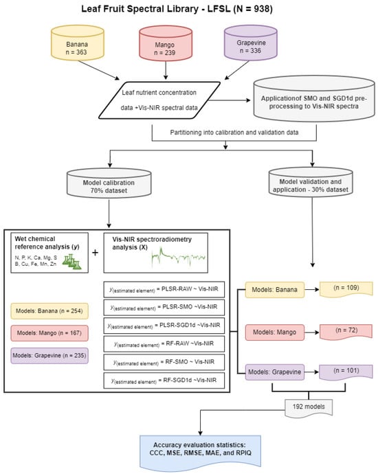
Figure 1.
Flowchart of the steps taken to organize the LFSL, calibrate and validate the models for predicting nutrient levels of N, P, K, Ca, Mg, S, Cu, Zn, Fe, Mn and B in banana, mango and grapevine leaves. PLSR: Partial Least Squares Regression; RF: Random Forest; RAW: original spectra; SMO: smoothed spectra; SGD1d: spectra with the 1st Savitzky–Golay derivative; CCC: concordance correlation coefficient; MSE: mean squared error; RMSE: root mean-square error; MAE: mean absolute error; RPIQ: ratio of performance to interquartile distance.
2.2. Leaf Sampling
The plants were randomly sampled in the orchards, following the leaf collection recommendations for each crop. Sampling was carried out on adult banana trees between 4 and 10 years old of the Cavendish subgroup variety (Nanica). The third youngest leaf was collected by taking a sub-sample from the middle part of the leaf, 10 cm long from the inside of the limb, removing the central vein [19]. Sampling takes place during the period from the time the bunch is issued until the inflorescence has all the female leaflets without bracts and two or three male leaflets open. Sampling was carried out on adult mango trees between 5 and 14 years old of the varieties ‘Keitt’, ‘Kent’ and ‘Tommy Atkins’. Mango leaves were collected by taking leaves from the middle third of newly mature branches (4 to 7 months old), in four quadrants, during the period when irrigation was suspended until flowering [20]. The grapevines were sampled from the cultivars ‘Chardonnay’, ‘Pinot Noir’ and ‘Isabel’ in 15-year-old vineyards. Sampling was carried out by collecting 8 complete leaves (limbus + petiole) in the position opposite the bunch, which were located in the middle third of the plant [3], during the period of full bloom and berry color change, forming a database (Figure 1). The samples were placed in paper bags, transported to the laboratory, and washed with distilled water, a 1% HCl solution, and distilled water. Subsequently, the samples were oven-dried at 65 °C, then ground and stored in low-density polyethylene bags. With the databases established, a total of 192 prediction models were generated at the end of the analyses, comprising 66 models for banana, 66 models for mango, and 60 models for grape (Figure 1).
2.3. Chemical Analysis
The grapevine samples were washed in the laboratory with distilled water, dried in an oven at 65 °C for 72 h and ground. The samples were prepared by subjecting them to sulphuric digestion [8] in a digestion block (Tecnal, Micro 42, Piracicaba, Brazil). N was determined by using the Kjeldahl drag steam distillation method (TE-0364, Tecnal, Piracicaba, Brazil).
The banana and mango tree samples were washed in distilled water, detergent solution (0.1%), hydrochloric acid solution (0.3%) and deionized water. The samples were then dried in an oven at 60/65 °C until they reached a constant weight, ground and subjected to sulphuric digestion [9]. Subsequently, N was determined by using the Kjeldahl steam distillation method.
Samples of grapevines were subjected to nitroperchloric digestion [9] and samples of banana and mango trees were subjected to nitroperchloric digestion [8]. All the macronutrients (N, P, K, Ca, Mg and S) and micronutrients (B, Cu, Fe, Mn and Zn) were determined in the chemical digestion extracts of each crop, except for grapevines, where S and B were not determined. The elements in the extracts were determined using the same methods for all the samples. The P levels was determined using the colorimetry method [21] at 882 nm on a spectrophotometer (SF325NM, Bel Engineering, Monza, Italy). K was determined using a flame photometer (B262 Micronal, São Paulo, Brazil). The levels of Ca, Mg, Mn, Fe, Cu and Zn were determined using an atomic absorption spectrophotometer (AAS; Perkin Elmer, Waltham, MA, USA, AAnalyst 200). B was determined using the dry combustion method [22]. B was determined at 435 nm using a spectrophotometer (SF325NM, Bel Engineering, Monza, Italy). S was determined using the turbidimetry method [8] with a spectrophotometer (SF325NM, Bel Engineering, Monza, Italy).
2.4. Vis-NIR Spectroscopy Readings and Spectral Pre-Processing
Leaf samples were oven-dried at 60–65 °C, ground and sieved at 1 mm, and subjected to spectral reflectance measurements in the Vis–NIR region (350–2500 nm) using a FielSpec® 4 spectroradiometer (Analytical Spectral Devices, Boulder, CO, USA) (Figure 2). The instrument provides a spectral resolution of 3 nm for 350–1000 nm and 8 nm for 1000–2500 nm, with sampling intervals of 1.4 nm and 2 nm, respectively. Approximately 10 cm3 of sample was placed in 4 cm diameter Petri dishes for measurement (Figure 2). All readings were performed in a laboratory, in a dark room, at an ambient temperature of 25 °C to ensure stable illumination and minimize external interference. Samples were rotated during spectral acquisition to improve measurement uniformity, and a standard white Spectralon® reference plate was scanned every 25 samples for sensor calibration.
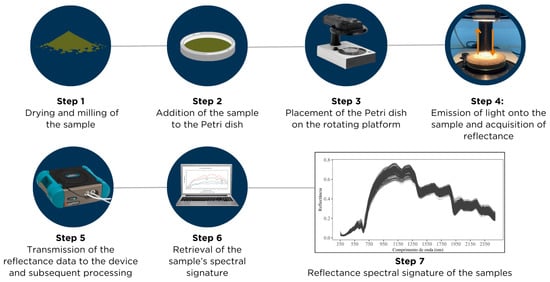
Figure 2.
Illustrative diagram of the procedure for reading plant tissue samples using the FieldSpec spectroradiometer (Analytical Spectral Devices, Boulder, CO, USA).
The original spectral data (RAW) was subjected to pre-processing, which consists of applying techniques to minimize interference in the spectra caused by light scattering from the equipment, sample variability and ambient light. Two pre-processing techniques were applied to the RAW spectra of the three crops: Smoothed (SMO) and Savitsky-Golay 1st derivative (SGD1d). The average spectral curves for the raw and pre-processed spectral data of the leaf samples from the three crops are presented in the Supplementary Material, Figure S1. These techniques are widely used to remove shifts from the baseline and highlight spectral features of interest [23], which has shown better results for nutrient prediction in leaves [10]. SMO is a technique used to smooth raw spectral curves by applying a moving average [24]. SGD1d involves the application of the first derivative using a first-order polynomial with a 9 nm window [24]. This technique is employed because it allows for the removal of baseline shifts and highlights reflectance features along the spectrum [23]. All the pre-processing of the spectra was carried out in the R programming language [25], using the prospectr package—version 0.2.8 [26].
2.5. Statistical Analysis and Calibration of Prediction Models
The nutrient concentration (N, P, K, Ca, Mg, S, B, Cu, Fe, Mn and Zn) obtained from the chemical analyses (sulphuric and nitroperchloric digestion), raw spectral data (RAW) and submitted to the SMO and SGD1d pre-processing techniques were combined in the LFSL (N = 938), which consisted of three crops: grapevine (n = 336), mango (n = 239) and banana (n = 363) (Figure 1). Initially, a descriptive statistical analysis (minimum, mean, maximum and standard deviation—SD) was carried out to characterize the variance of the nutrient concentration from the chemical analysis in the leaves of each crop.
Prediction models were developed to predict the levels of N, P, K, Ca, Mg, S, B, Cu, Fe, Mn and Zn in the leaf for the three crops, combining two machine learning methods and three spectral pre-processing techniques, totaling 192 prediction models (Figure 1). The machine learning methods used to calibrate the models were: Partial Least Squares Regression (PLSR), a parametric linear method that reduces the dimension of the data and increases the covariance between the variables, forming a statistical model that relates matrices of “x” and “y” variables [27]. PLSR has the ability to reduce data dimensionality by projecting the spectral bands onto a set of latent variables and assigning greater weight to those bands that contribute most to the prediction [28]. The second model was Random Forest (RF), a non-parametric method for combining decision trees, where the prediction of each tree is independent [29]. The RF model can handle high-dimensional datasets directly and is also capable of identifying the most important predictor variables. In this study, RF was implemented with the recursive feature elimination (RFE) procedure to select the most informative predictors [29]. Among the calibration methods, the PLSR method is widely used for quantitative analysis, mainly generating prediction models with spectral reflectance data from plant tissue samples [27]. On the other hand, the RF method shows better results when the database does not have a normal distribution [29].
The LFSL of each crop was separated into 70% of the samples for calibration and 30% for validation (Figure 1). The validation phase was carried out with the aim of simulating the application of the models in real-world situations. This approach was used to assess model generalization and identify potential overfitting [29,30,31]. The calibration and validation process was conducted in R [25] using the ‘caret’ package—version 7.0-1 [32]. For the PLSR model, the ncomp parameter (number of principal components) was optimized through cross-validation using the bestTune function. In the RF model, the hyperparameters ntrees (number of trees) and mtry (number of predictor variables considered at each split). The cross-validation procedure used for hyperparameter tuning involved random partitioning of the datasets into k = 10 subsets [33].
The metrics used to evaluate the performance and accuracy of the prediction models were concordance correlation coefficient (CCC), mean squared error (MSE), root mean square error (RMSE), mean absolute error (MAE), ratio of performance to interquartile distance (RPIQ). The CCC metric simultaneously assesses precision and accuracy and is widely used to compare observed vs. predicted values [34]. In this sense, when the CCC value is close to zero, it means that there is no relationship between the spectral reflectance data and the reference data; when the CCC value is close to 1, it shows that the data are highly related to each other. The MSE and RMSE analyze the differences between the reference values and the estimated values and assesses accuracy by comparing the prediction errors between the models [35,36], but MSE is less sensitive to extreme values than the RMSE, as it penalizes large errors. The MAE is the average difference between the reference data and the estimated data [37]. The RPIQ takes into account the prediction error in relation to the variation in the estimated values [37]. Therefore, to obtain a model with high performance and accuracy, the CCC and RPQI values need to be high and the MSE, MAE and RMSE values low.
Analysis of variance (ANOVA) was applied to the CCC values obtained by the prediction models and, when significant, the CCC means of the machine learning methods, pre-processing techniques and nutrient were compared using the Scott–Knott test (p < 0.05). All the analyses were implemented in the programming language R [25]. Finally, nutrient concentrations obtained by chemical digestion methods (sulfuric and nitroperchloric) and by the Vis–NIR method (estimates from the most accurate models) were interpreted using established reference values for banana [38], mango [39], and grapevine [3]. Nutrient concentrations were classified into three categories—Insufficient, Normal, and Excessive—for each crop. This classification step was conducted to assess the practical applicability of the results for real-world crop nutritional diagnosis based on nutrient concentrations estimated by Vis–NIR predictive models.
3. Results
3.1. Descriptive Statistical Analysis of the Database
The descriptive statistical analysis showed differences in the variation in nutrient concentration among the three fruit leaf spectral libraries (LFSL), ‘Banana’, ‘Mango’ and ‘Grapevine’, with greater amplitudes and standard deviations observed in micronutrients (Table 1, Table 2 and Table 3). The Mn concentrations present in the samples showed greater amplitudes in the ‘Banana’ LFSL (18 to 745 mg kg−1 and SD of 161.20 mg kg−1) (Table 1) and ‘Mango’ (25 to 123.39 mg kg−1 and SD of 222.98 mg kg−1) (Table 2). Similarly, Fe concentrations also showed a wide range of values (Table 1, Table 2 and Table 3).

Table 1.
Descriptive statistics of nutrient levels in leaves from the banana database.
Table 2.
Descriptive statistics of nutrient levels in leaves from the mango database.
Table 3.
Descriptive statistics of nutrient levels in leaves from the grapevine database.
Among the macronutrients, N and K showed the greatest variation, with the highest standard deviation values observed in the “Banana” leaf sample (Table 1), compared to the other LFSL. The P, Mg and S levels obtained from the leaf samples of banana and mango trees showed the smallest ranges compared to the other nutrients, with P having the smallest range for the ‘Banana’ LFSL (0.64 to 3.34 g kg−1 and SD of 0.30 g kg−1) (Table 1) and S having the smallest range for the ‘Mango’ LFSL (0.15 to 1.29 g kg−1 and SD of 0.28 g kg−1) (Table 2). In the ‘Grapevine’ LFSL, the S levels were not estimated, and the P, K and Mg levels showed the smallest ranges, with Mg being the smallest (1.10 to 2.77 g kg−1 and SD of 1.07 g kg−1) (Table 3).
3.2. Calibration and Validation Performance of Prediction Models
Detailed statistics from the calibration stage of the prediction models are presented in Supplementary Tables S1–S3. In general, the highest calibration accuracy is observed for the “Grapevine” LFSL model, followed by the mango and banana LFSL models (Tables S1–S3). The “method + preprocessing” combinations PLSR-SMO, RF-SMO, PLSR-SGD1d, and RF-SGD1d showed better performance compared to PLSR+RAW and RF-RAW, where models are calibrated with raw spectra—without preprocessing.
In the testing (validation) stage in real-world situations, the accuracy assessment was based on the CCC and MSE values derived from each model, which showed differences in sugar content among the three LFSLs, as well as macronutrients and micronutrients (Figure 3 and Figure 4). Among the macronutrients, Ca, Mg, and P showed the highest accuracy in predictions across the three LFSLs and in all “method + preprocessing” combinations, with CCC values > 0.75 and MSE < 2 g kg−1 (Figure 3 and Figure 4). The lowest accuracies were observed in K predictions, with high CCC values, but also high MSE values. Among the micronutrients, Fe showed the lowest accuracy in predictions across all three LFSL and in all “method + preprocessing” combinations, with CCC values < 0.60 and MSE > 50 mg kg−1 (Figure 3 and Figure 4). The highest accuracies were observed in the predictions of B and Cu, with high CCC values (>0.80), but also high MSE values.
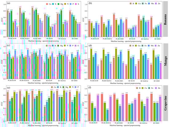
Figure 3.
Comparison of concordance correlation coefficient (CCC) values obtained in the validation stage of macronutrient (a,c,e) and micronutrient (b,d,f) prediction models combining machine learning methods and pre-processing in the LFSL of ‘Banana’, ‘Mango’ and ‘Grapevine’.
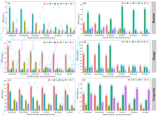
Figure 4.
Comparison of mean squared error (MSE) values obtained in the validation stage of macronutrient (a,c,e) and micronutrient (b,d,f) prediction models combining machine learning methods and pre-processing in the LFSL of ‘Banana’, ‘Mango’ and ‘Grapevine’.
In the LFSL ‘Banana’, Ca and Mg were the nutrients with the highest CCC values (>0.80) and lowest MSE values (<1.5 g kg−1) (Figure 3a and Figure 4a, respectively) in the “method + preprocessing” combinations PLSR-SMO, RF-SMO, PLSR-SGD1d, and RF-SGD1d. Predictions of K and N show high CCC values (>0.70), but with high MSE values (>10.0 for K g kg−1 and >6.0 for N g kg−1) (Figure 4a). The prediction models for micronutrients in the LFSL ‘Banana Tree’ showed low CCC values (≤0.70) in all combinations (Figure 3b) and high MSE values (Figure 4b), especially for Fe.
In the ‘Mango’ LFSL, P was the nutrient that showed the highest accuracy of all macronutrients, in all combinations, with CCC values > 0.85 (Figure 3c). Next came K, with CCC values ≥ 0.80 (Figure 3c). In the micronutrient models, Cu was the nutrient with the best precision in all combinations, with CCC values ≥ 0.90 (Figure 3d). Mn also showed good results in the ‘Mango’ LFSL, with CCC values ≥ 0.80 (Figure 3d).
In the LFSL ‘Grapevine’ sample, the macronutrients with the best results were N and Ca, with CCC values ≥ 0.90 (Figure 3e), but high MSE values (>4.0 g kg−1) (Figure 4f). The Mg prediction reached CCC values > 0.70 (Figure 3e) and low MSE values (<1.0 g kg−1) (Figure 4e). Among micronutrients, B showed the highest CCC (≥0.80), but with high MSE values (>50 mg kg−1). Fe predictions showed the lowest accuracy, lowest CCC values (<0.50) and highest MSE values (>80 mg kg−1) (Figure 4f).
The LFSLs of ‘Banana’, ‘Mango’, and ‘Grapevine’ were compared using the Scott–Knott mean test, evaluating the PLSR and RF machine learning methods. The results of the statistical analysis showed that the ‘Grapevine’ LFSL presented prediction models with better accuracy when compared to the other LFSLs, and the PLSR and RF methods were not significantly different (Figure 5a). However, the SMO and SGD1d spectral preprocessing did not show significant differences between the LFSLs, but there was a significant difference in the models generated with RAW, with inferior performance when compared to the models calibrated with preprocessed data (Figure 5b).
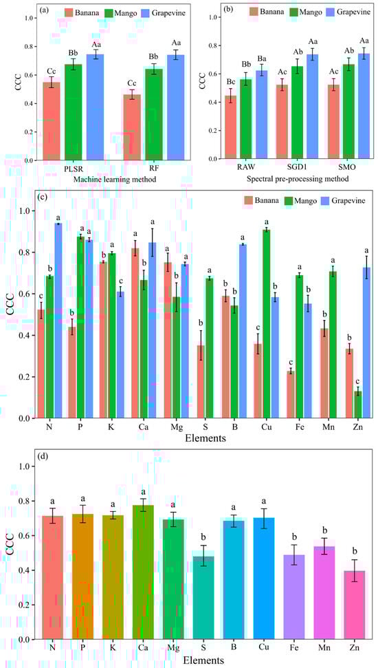
Figure 5.
Comparison of the performance of machine learning methods (a) spectral pre-processing (b), crop-predicted elements (c) and crop-independent elements (d) indicated by the concordance correlation coefficient (CCC) values in the model validation stage. In figures “(a)” and “(b)”, lowercase letters compare values between crops using the same machine learning method, and uppercase letters compare machine learning methods within the same crop using the Scott–Knott test (p < 0.05). In figure “(c)”, lowercase letters compare the values of each nutrient between crops using the Scott–Knott test (p < 0.05). In figure “(d)”, lowercase letters compare values between nutrients using the Scott–Knott test (p < 0.05).
When evaluating the nutrient models by crop, the average CCC of the models was compared between the ‘Banana’, ‘Mango’, and ‘Grapevine’ LFSLs, showing the difference between them, using the Scott–Knott mean test (Figure 5c). Mg showed a significant difference between the LFSLs, with the best performance in ‘Banana’ and ‘grapevine’, with a CCC value > 0.75. The lowest accuracies in the ‘Banana’ LFSL were observed for N, P, S, and Fe, with CCC values < 0.55 (Figure 5c). The nutrients P, K, S, Cu, Fe, and Mn showed significantly better results in the ‘Mango’ LFSL, with CCC values > 0.75. Calcium was the element with the lowest predictive capacity in the ‘Mango’ LFSL, with a CCC value < 0.7 (Figure 5c). In the LFSL ‘Grapevine’, N and Ca showed better accuracy, with CC values > 0.85, as did B and Zn, with CC values > 0.75 (Figure 5c). However, the K nutrient showed inferior performance in terms of predictive capacity in the LFSL of the ‘Grapevine’ variety compared to the others, with CCC values < 0.70 (Figure 5c).
In general, the nutrient prediction models presented average CCC values < 0.8. N, P, K, Ca, and Mg were the models with the greatest estimation capacity, with average CCC values > 0.70 (Figure 5d). S, Fe, Mn, and Zn were the nutrients with the lowest predictive capacity in the validation models, with an average CCC < 0.55 (Figure 5d).
The highest MSE values for macro and micronutrients were observed in the LFSL ‘Banana’ and ‘Mango’ predictions, while the lowest values were achieved for LFSL ‘Grapevine’, particularly for micronutrients (Figure 6). This result, combined with the observed CCC values (Figure 5), shows the greater accuracy in nutrient predictions for the LFSR ‘Grapevine’ dataset.
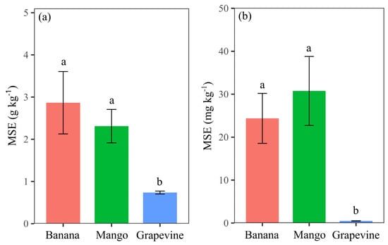
Figure 6.
Average MSE values of macronutrient (a) and micronutrient (b) predictions obtained in the model validation stage for the three fruit crops. Lowercase letters compare values between crops using the Scott–Knott test (p < 0.05).
To evaluate the applicability of the results in real-world situations, the nutrient values obtained by the nitroperchloric digestion methods and estimated by the Vis-NIR prediction models were interpreted using the reference values for each nutrient and crop. The results are presented in Table 4, Table 5 and Table 6, where it is possible to observe that the proportion of samples falling into the three classes (insufficient, normal, excessive) is similar. In general, across the three crops and all elements, differences in nutritional classification among the three classes (insufficient, normal, and excessive) were ≤5%. For example, in banana, 40%, 48%, and 12% of the samples were classified as insufficient, normal, and excessive, respectively, based on nutrient concentrations determined by chemical digestion (Table 1). A similar distribution was obtained using N concentrations estimated by the Vis–NIR model, with 42%, 54%, and 4% of the samples classified as insufficient, normal, and excessive, respectively.
Table 4.
Interpretation of nutrient levels obtained through nitroperchloric and sulfuric chemical digestion and Vis-NIR predictive models, classified as Insufficient, Normal, and Excessive based on reference values for banana trees.
Table 5.
Interpretation of nutrient levels obtained through nitroperchloric and sulfuric chemical digestion and Vis-NIR predictive models, classified as Insufficient, Normal, and Excessive based on reference values for mango trees.
Table 6.
Interpretation of nutrient levels obtained through nitroperchloric and sulfuric chemical digestion and Vis-NIR predictive models, classified as Insufficient, Normal, and Excessive based on reference values for grapevines trees.
4. Discussion
The LFSL used to develop the prediction models showed a high range of levels for most of the nutrients (Table 1, Table 2 and Table 3). Levels variation is an important factor for model development, as it allows for a wider prediction range (prediction interval) [10,11,27]. However, databases with larger prediction intervals can present greater variance (>standard deviation) in nutrient levels, which can lead to a reduction in the accuracy of model predictions [10,11,37]. In general, greater amplitude and variation in micronutrient concentration were observed, which is characteristic of micronutrient analysis in fruit tree leaves [40]. This greater variation led to lower accuracy in micronutrient prediction, with higher MSE values (Figure 6), especially for the ‘Banana’ and ‘Mango’ LFSL, which showed the greatest variations in concentrations. This same behavior in the accuracy of Vis-NIR models in prediction due to greater variation in the target variable was also observed in the prediction of nutrients in Ilex paraguariensis [10] and soil organic carbon [41,42].
In this study, Mn stands out for having the widest prediction intervals and high SD values in the three crops (Table 1, Table 2 and Table 3). In the LFSL of ‘Grapevine’, Mn obtained the highest SD value (262.79 mg kg−1), compared to the other crops (Table 3). This may have been due to the presence of Mn on the leaf surface, caused by applications of fungicides such as Mancozeb (manganese ethylenebis (dithiocarbamate) (polymeric) complex with zinc salt) (C4H6N2S4Mn)x (Zn)y [43]. In viticulture, mancozeb is the main contact fungicide for the control of downy mildew (Plasmopara viticola) [44], being a foliar-applied product with low water solubility. This characteristic may explain the variance in Mn levels in the grapevine leaf samples, since the samples were washed only with water. Thus, the washing method may be an interfering factor in the Mn prediction models. However, this explanation does not extend to the LFSL of ‘Banana’ and ‘Mango’, because even with high SD values (161.20 and 222.98 mg kg−1, respectively) (Table 1 and Table 2), no applications of mancozeb or any other Mn-based product were made via foliar application.
The models generated to predict N showed different responses for banana, mango, and grapevine (Figure 5c). The calibrated LFSL models for ‘Banana’ and ‘Mango’ showed the lowest precision in the estimates, with average CCC values < 0.70 (Figure 5c) and MSE values greater than 4.0 g kg−1 (Figure 5a and Figure 5c, respectively; Tables S1 and S2). The results observed in this study were lower than those described in the literature for other crops, where R2 ranged from 0.91 to 0.99 [10,41]. The LFSL models for ‘Grapevine’ showed greater precision, with CCC values > 0.90 (Figure 3e) and MSE ≤ 4.0 g kg−1 (Figure 4e and Table S3), in line with some of the values described in the literature [12,13]. The sets of leaf samples that make up the LFSL used in the modeling for the three crops show differences in fertilization management, with banana and mango being subjected to fertigation and grapevine not. This leads to a variation in the N element in the leaf, with greater variation in N observed in the banana and mango LFSL leaves (Table 1 and Table 2, respectively), which led to the lower predictive performance of the models. In addition, greater variability in N concentration is expected in banana leaves [38], owing to their large leaf size and the representativeness of the sampled tissue, which consisted of a 10 cm-long subsample taken from the central portion of the leaf [19].
The P levels showed little variation in the crops, with SD values of 0.30, 0.91 and 3.19 g kg−1 for ‘Banana’, ‘Mango’ and ‘Grapevine’, respectively (Table 1, Table 2 and Table 3). The low variation may be related to the small response of most fruit species to phosphate fertilization in the adult phase, with P being absorbed in smaller quantities compared to other nutrients, as the amount exported by the fruit is usually low [2]. The performance of the P prediction models obtained good results, with average values of CCC > 0.85 in the ‘Mango’ LFSL and CCC > 0.80 in the ‘Grapevine’ LFSL (Figure 5c), values close to those observed in the literature for the orange crop, where a value of R2 = 0.77 was obtained [6] and for Ilex paraguariensis with values of R2 > 0.70 [10]. However, for the LFSL of ‘Banana’, the P models showed low accuracy, with an average value of CCC < 0.50, i.e., values lower than those found in the literature for eucalyptus [45], orange [6] and Ilex paraguariensis [10] (Figure 5c).
The results for Ca show that the models are better at predicting the nutrient; in general, of all the 11 nutrients evaluated, Ca had an average CCC > 0.65 (Figure 5d). By crop, this nutrient obtained superior results in the LFSL of ‘Grapevine’, followed by ‘Banana’, with average values of CCC > 0.85 and CCC > 0.80, respectively (Figure 5c). However, the MSE values varied considerably between crops, where MSE < 2.0 g kg−1 was observed for banana, >6.0 g kg−1 for mango and >8.0 g kg−1 for grapevine (Figure 4a, Figure 4c and Figure 4e, and Tables S1, S2, S3, respectively). The higher MSE values observed in the prediction of Ca in Grapevine leaves are explained by the higher standard deviation of the Ca concentration (Table 3), which leads to a reduction in the accuracy of the estimates [10,37]. These accuracy results observed in the model predictions were superior to those obtained for orange trees [6], but inferior to the models generated for yerba mate [10]. The greater accuracy of the estimates of the Ca models can be explained by the presence of Ca in the structural composition of the middle lamella of the cell wall, mainly in the form of Ca pectates [46]. Also, the nutrient has low levels in the phloem and low solubility of its compounds, resulting in a low redistribution of Ca and stable levels in the leaves sampled [40].
The K predictions showed inferior performance for LFSL ‘Banana’, despite high CCC values > 0.80 (Figure 5c), showing high MSE values > 10 g kg−1 (Figure 4a and Table S1). For the LFSL ‘Grapevine’ set, the accuracy was intermediate, with CCC values > 0.65 and MSE > 5.0 g kg−1 (Figure 4e and Table S3). The accuracy results observed in this study are similar to those observed in the literature for different crops, such as eucalyptus, Ilex paraguariensis, and citrus, where R2 values vary from 0.76 to 0.99 for K [10,15,45], respectively]. The highest accuracy in K predictions was observed for the LFSL ‘Mango’, which reached CCC values > 0.60 and MSE < 1.0 g kg−1 (Figure 4c and Table S2). This variation in K prediction among crops is explained by the variation in the element’s concentration in the leaves, where the greatest variation (SD = 6.72 g kg−1, Table 1) is observed in banana, resulting in reduced prediction accuracy. Another explanation for the variation in the performance of prediction models for K may be linked to the chemical form in which the nutrient is present in the plant. K is found in ionic form (K+), i.e., it does not constitute any cellular structure and is not bound to any organic compound in the plant [40]. Little is known about how models are able to predict K, since it is not present in structures or molecules to be detected in spectral reflectance readings. In plants, high levels of K are localized in the cytoplasm and chloroplasts, when nutrient levels are adequate for the crop [40]. In this case, it may be that K is detected by the high levels in these locations.
The models for predicting Mg show good performance in the three LFSL with high CCC values > 0.80 (Figure 5c) and low MSE values < 1.0 g kg−1 (Figure 4a,c,e and Tables S1–S3). This is explained by the low range and standard deviation observed in the Mg concentration in the three crops (Table 1, Table 2 and Table 3), reflecting the behavior of the nutrient in the plant, which generally shows low variation [40].
The prediction models for Fe performed poorly for the three crops, obtaining an average value of CCC < 0.75 (Figure 5d) and high MSE values > 80 mg kg−1 (Figure 4b,d,f and Tables S1–S3). The Fe levels in the samples used in the LFSL had a high amplitude (Table 1, Table 2 and Table 3), which can be explained by the possible variation in the soil’s physicochemical attributes, such as clay minerals, Fe oxides and hydroxides in the sampling regions [5]. On the other hand, the chemical form of Fe can interfere with the spectral reading of the sample. Fe is stored in plants in the form of phytoferrimite (FeO.OH)8 (FeOOPO3H2). This reserve is located in the stroma of plastids in cells [40]. The possibility is that the Vis-NIR spectral range (350 to 2500 nm) does not easily detect Fe in the form of phytoferrimite. In comparison with the literature, a study carried out with Ilex paraguariensis obtained prediction models with a value of R2 = 0.98, using to read the samples with a mid-infrared spectroradiometer (MIR) in the (2500 to 18,000 nm) range [10], which may be the most suitable wavelength range for predicting Fe.
Nutrients such as Cu and Zn showed high ranges of levels in the samples, but with less variation when compared to the other micronutrients such as Fe and Mn (Table 1, Table 2 and Table 3). In grapevines, the variations come from phytosanitary control, i.e., successive applications of Cu-based fungicides such as Bordeaux mixture [Ca(OH)2 + CuSO4] and copper oxychloride [CuCl23Cu(OH)2] and Zn-based fungicides such as mancozeb which, over time, increase the levels of these elements in the soil [47]. This is also true for banana trees, because when disease control is carried out, there may be an increase in these nutrients in the soil and a residual in the leaves. The mango trees received three applications of copper sulphate (CuSO4) to control fungal diseases. In addition, Zn deficiency is common and, for this reason, applications of the nutrient can be made via soil or foliar [48].
The models for predicting Mn show poor performance in the “Banana” and “Mango” leaf, with CCC values < 0.50 and <0.75, respectively (Figure 5c), and high MSE values, >10 mg kg−1 and >25 mg kg−1 (Figure 4b and Figure 4d and Tables S1 and S2, respectively). This is explained by the high range and standard deviation observed in the Mn concentration in the leaves of these crops (Table 1 and Table 2), with standard deviation values > 150 mg kg−1.
S showed low amplitude and low levels of the nutrient (Table 2). These characteristics in the sample set may have had a negative influence on the prediction of S, since the models obtained an average CCC value close to 0.40 for LFSL ‘Banana’ (Figure 4d) and MSE > 0.10 g kg−1 (Figure 4b and Table S1). For the LFSL “Mango” the CCC value was higher, close to 0.75, but the MSE values were 0.75 g kg−1 (Figure 4d and Table S2). However, the reference method used to determine S, as described by [8], also shows low levels when the samples are analyzed. In this case, if the nutrient data obtained by the reference methods (e.g., sulphuric and nitroperchloric digestion) are of poor quality in the extraction and determination process, this could negatively interfere in the correlation process with Vis-NIR data in the calibration of the prediction models, resulting in a reduction in the accuracy of the models.
In the LFSL of ‘Mango’, B showed a high amplitude in levels in the leaf samples, with a SD of 14.99 mg kg−1 (Table 2). This variation interfered negatively with the performance of the prediction models, which reached values of CCC < 0.60 (Figure 3d) and MSE > 80 mg kg−1 (Figure 4d). In mango growing, B deficiency is one of the main micronutrients. Correction can be carried out via the soil, by applying fertilizers, or via foliar application, by spraying solutions of boric acid (H3BO3) or borax Na2[B4O5(OH)4] 8H2O, as a source of B [48].
When evaluating the PLSR and RF methods used to calibrate and validate the models, the results showed that there was no significant difference between them, but LFSL ‘Grapevine’ was the best among the three crops (Figure 5a). This result is explained by the lower standard deviation observed in the nutrient concentration of LFSL ‘Grapevine’, which led to greater accuracy in the predictions by the predictive models, corroborating results observed in other studies [10,42].
Regarding RAW, SMO, and SGD1d preprocessing, the results showed that the models with pre-processed spectral readings were better at predicting nutrients than the models with raw spectral readings, regardless of LFSL (Figure 5b). In comparison with the reading, several studies have shown that the use of pre-processing in spectral readings helps to obtain models with better accuracy [6,10,12,13,15,16].
In general, the performance of the models showed moderate accuracy for most models (Figure 5d). The observed results may be influenced by factors related to variation (standard deviation) in the concentrations of nutrients present in the LFSL [10,42]. Also, the number of observations used in the study were n = 363 in the ‘Banana’ LFSL, n = 239 in the ‘Mango’ LFSL and n = 336 in the ‘Grapevine’ LFSL. When the number of observations in the database is small, less than 500, this can interfere with the calibration of the models, along with high standard deviation values [2]. Leaf sampling methods can also have a negative influence when they are not representative of the nutrient contents present in the leaves. The chemical digestion reference methods used are other factors that may be influential, as the methods present analytical problems, such as the low precision of laboratory measurements and the absence of any replication in the analysis. Ref. [49], which influences the calibration of the models, as already discussed. In addition, the low levels of nutrients in the samples can reduce the accuracy of the prediction models [1], as, for example, in the P and S models generated in this study (Figure 5d).
Regarding the interpretation of nutrient levels into classes (Insufficient, Normal, and Excessive) based on the reference values for each crop [3,38,39], the results were similar between the nitroperchloric-sulfuric digestion and the best Vis-NIR prediction models for each nutrient and crop (Table 4, Table 5 and Table 6). This indicates that the nutrient levels obtained through Vis-NIR prediction models are consistent with traditional methods.
Thus, the results obtained in this study show that the use of Vis-NIR hyperspectral sensors to quantify the spectral reflectance of plant tissue samples (leaves), together with the combination of machine learning methods and spectral pre-processing, has the potential to estimate the contents of N, P, K, Ca, Mg, S, Cu, Zn, Fe, Mn and B. However, new calibration studies need to be carried out using more robust databases, with different sampling methods and sample preparation. Other machine learning methods, pre-processing and mid-infrared spectroscopy (MIR) should also be evaluated. In this way, it will be possible to develop more robust protocols for using spectroscopy as an alternative method to reference methods for estimating plant nutrients more quickly and sustainably. Finally, the results of this study have provided information for future research into the use of Vis-NIR hyperspectral sensors in leaf nutrient estimation and the development of protocols for expanding the use of the technique in commercial laboratories in the future. In addition, the findings showed the effect that variations in nutrient concentrations have on the accuracy of Vis-NIR model predictions, which is important information for compiling LFSLs intended for the calibration of predictive models based on Vis-NIR spectral data.
5. Conclusions
The Vis-NIR spectroscopy method has the potential to be an alternative method to the sulphuric and nitroperchloric digestion methods for estimating nutrients in banana, mango and grapevine leaves.
Leaf spectral reflectance data obtained via Vis-NIR spectroscopy, together with combinations of the PLSR and RF machine learning methods and SMO and SGD1d pre-processing, had a positive influence, generating highly accurate models (CCC > 0.80 and MSE < 2 g kg−1) for Ca in the ‘Banana’ LFSL, P and Cu in the ‘Mango’ LFSL, and N and Ca in the ‘Grapevine’ LFSL.
The PLSR and RF machine learning methods did not differ in terms of estimation accuracy. Models calibrated with spectra subjected to the SMO and SGD1d pre-processing techniques had the highest accuracies compared to models calibrated with unprocessed spectra (RAW).
The predictive models calibrated for the LFSL of ‘Grapevine’ exhibited the highest accuracy—characterized by higher CCC values and lower MSE values—when compared with the LFSL models developed for ‘Mango’ and ‘Banana’. The high amplitudes and variations in nutrient concentration, together with the high standard deviations, negatively influenced the ability of the prediction models, particularly the ‘Banana’ and ‘Mango’ LFSL models.
Supplementary Materials
The following supporting information can be downloaded at: https://www.mdpi.com/article/10.3390/horticulturae12010108/s1, Figure S1. Average spectral curves and standard deviation (buffer in gray) referring to the RAW and pre-processed (SMO and SGD1d) spectral data of leaf samples from the three crops—Banana, Mango, and Grapevine. Table S1. Accuracy of nutrient concentration predictions in banana leaves during the calibration (CCCc, MSEc, RMSEc, MAEc e RPIQc) and validation (CCCv, MSEv, RMSEv, MAEv e RPIQv) stages of the models. Table S2. Accuracy of nutrient concentration predictions in mango leaves during the calibration (CCCc, MSEc, RMSEc, MAEc e RPIQc) and validation (CCCv, MSEv, RMSEv, MAEv e RPIQv) stages of the models. Table S3. Accuracy of predictions of nutrient concentration in grapevine leaves during the calibration (CCCc, MSEc, RMSEc, MAEc e RPIQc) and validation (CCCv, MSEv, RMSEv, MAEv e RPIQv) stages of the models.
Author Contributions
Conceptualization, A.M.C., J.M.M.-B. and G.B.; methodology, A.M.C., C.A.M. and M.d.S.S.; investigation, A.M.C., C.A.M., M.d.S.S., C.M., D.L.G. and A.T.; writing—review and editing, A.M.C., J.M.M.-B., C.M., W.N., D.E.R. and G.B.; visualization, A.M.C. and J.M.M.-B.; supervision, J.M.M.-B. and G.B.; project administration, A.M.C. and G.B. All authors have read and agreed to the published version of the manuscript.
Funding
This research received no external funding.
Data Availability Statement
The raw data supporting the conclusions of this article will be made available by the authors on request.
Acknowledgments
We are grateful to Coordenação de Aperfeiçoamento de Pessoal de Nível Superior—CAPES (Coordination for the Improvement of Higher Education Personnel) for the research productivity scholarship, granted to the first author.
Conflicts of Interest
The authors declare that they have no conflicts of interest.
References
- Rozane, D.E.; Paula, B.V.; Santos, E.M.H.; Tullio, L.; Conceição, M.P.; Lima Neto, A.J.; Moura-Bueno, J.M.; Trapp, T.; Hahn, L.; Brunetto, G. Indication of critical levels and sufficiency ranges of nutrients in soil and plant tissue. In Management Strategies to Improve Nutrient Use Efficiency in Fruit Crops, 1st ed.; Brunetto, G., Rozane, D.E., Loss, A., Natale, W., Eds.; Editora Palotti: Santa Maria, CA, USA, 2023; pp. 15–28. [Google Scholar]
- Brunetto, G.; Nava, G.; Ambrosini, V.G.; Comin, J.J.; Kaminski, J. The pear tree response to phosphorus and potassium fertilization. Braz. J. Fruit Grow. 2015, 37, 507–516. [Google Scholar] [CrossRef]
- CQFS—RS/SC—Commission for Soil Chemistry and Fertility. Manual of Liming and Fertilization for the States of Rio Grande do Sul and Santa Catarina, 11th ed.; Brazilian Soil Science Society—Southern Regional Nucleus [s.l.]: Commission for Soil Chemistry and Fertility—RS/SC: Viçosa, Brazil, 2016. [Google Scholar]
- Tassinari, A.; Stefanello, L.O.; Schwalbert, R.A.; Vitto, B.B.; Kulmann, M.S.S.; Santos, J.P.J.; Arruda, W.S.; Schwalbert, R.; Tiecher, T.L.; Ceretta, C.A.; et al. Nitrogen Critical Level in Leaves in ‘Chardonnay’ and ‘Pinot Noir’ Grapevines to Adequate Yield and Quality Must. Agronomy 2022, 12, 1132. [Google Scholar] [CrossRef]
- Stefanello, L.; Schwalbert, R.; Schawlbert, R.; Tassinari, A.; Garlet, L.; De Conti, L.; Ciotta, M.; Ceretta, C.; Ciampitti, I.; Brunetto, G. Phosphorus critical levels in soil and grapevine leaves for South Brazil vineyards: A Bayesian approach. Eur. J. Agron. 2023, 144, 126752. [Google Scholar] [CrossRef]
- Osco, L.P.; Ramos, A.P.M.; Pinheiro, M.M.F.; Moriya, E.A.S.; Imai, N.N.; Estrabis, N.; Ianczyk, F.; Araújo, F.F.; Liesenberg, V.; Jorge, L.A.C.; et al. A Machine Learning Framework to Predict Nutrient Content in Valencia-Orange Leaf Hyperspectral Measurements. Remote Sens. 2020, 12, 906. [Google Scholar] [CrossRef]
- Souza, R.M.; Coelho, M.S.; Rodrigues, B.J. Development of a method to prepare plant material samples for determination of Ca, Cu, Mg, Mn, Fe and Zn by FAAS. Braz. Appl. Sci. Rev. 2020, 4, 1811–1821. [Google Scholar] [CrossRef]
- Tedesco, M.J. Analysis of Soil, Plants, and Other Materials, 2nd ed.; Soil Department, UFRGS: Porto Alegre, Brazil, 1995. [Google Scholar]
- EMBRAPA, Brazilian Agricultural Research Corporation. Manual of Chemical Analysis of Soils, Plants and Fertilizers; EMBRAPA: Rio de Janeiro, Brazil, 2009.
- Naibo, G.; José, J.F.B.d.S.; Pesini, G.; Chemin, C.; Lisboa, B.; Kayser, L.; Abichequer, A.D.; Moura-Bueno, J.M.; Ramon, R.; Tiecher, T. Combining mid-infrared spectroscopy and machine learning to estimate nutrient content in plant tissues of yerba mate (Ilex paraguariensis A. St. Hil.). J. Food Compos. Anal. 2024, 128, 106008. [Google Scholar] [CrossRef]
- Zhu, G.; Wang, Q.; Zhang, S.; Guo, T.; Liu, S.; Lu, J. A meta-analysis of crop leaf nitrogen, phosphorus and potassium content estimation based on hyperspectral and multispectral remote sensing techniques. Field Crops Res. 2025, 329, 109961. [Google Scholar] [CrossRef]
- Páscoa, R.N.M.J. In Situ Visible and Near-infrared Spectroscopy Applied to Vineyards as a Tool for Precision Viticulture. Compr. Anal. Chem. 2018, 80, 253–279. [Google Scholar] [CrossRef]
- Manzano, J.I.; Rodríguez-Febereiro, M.; Fandiño, M.; Vilanova, M.; Cancela, J.J. Spectroscopic analysis (UV-VIS-NIR) for predictive modeling of macro and micronutrients in grapevine leaves. Smart Agric. Technol. 2025, 10, 100812. [Google Scholar] [CrossRef]
- Galvez-Sola, L.; García-Sánchez, F.; Pérez-Pérez, J.G.; Gimeno, V.; Navarro, J.M.; Moral, R.; Martínez-Nicolás, J.J.; Nieves, M. Rapid estimation of nutritional elements on citrus leaves by near infrared reflectance spectroscopy. Front. Plant Sci. 2015, 6, 571. [Google Scholar] [CrossRef]
- Jin, X.; Wang, L.; Zheng, W.; Zhang, X.; Liu, L.; Li, S.; Rao, Y.; Xuan, J. Predicting the nutrition deficiency of fresh pear leaves with a miniature near infrared spectrometer in the laboratory. Measurement 2022, 188, 110553. [Google Scholar] [CrossRef]
- Azadnia, R.; Rajabipour, A.; Jamshidi, B.; Omid, M. New approach for rapid estimation of leaf nitrogen, phosphorus, and potassium contents in apple-trees using Vis/NIR spectroscopy based on wavelength selection coupled with machine learning. Comput. Electron. Agric. 2023, 207, 107746. [Google Scholar] [CrossRef]
- Cuq, S.; Lemetter, V.; Kleiber, D.; Levasseur-Garc, C. Assessing macro-element content in vine leaves and grape berries of vitis vinifera by using near-infrared spectroscopy and chemometrics. Int. J. Environ. Anal. Chem. 2019, 100, 1179–1195. [Google Scholar] [CrossRef]
- Xiao, H.; Li, C.; Wang, M.; Huan, Z.; Mei, H.; Nie, J.; Rogers, K.M.; Wu, Z.; Yuan, Y. Nutrient Content Prediction and Geographical Origin Identification of Bananas by Combining Hyperspectral Imaging with Chemometrics. Foods 2024, 13, 3631. [Google Scholar] [CrossRef]
- Martin-Prével, P. International colloquium for optimizing plant nutrition. Proceedings 1984. [Google Scholar]
- Silva, D.J.; Wadt, P.G.S.; Mouco, M.A.C. Foliar diagnosis of mango crop. In Plant Nutrition: Foliar Diagnosis in Fruit Crops; Prado, R.d.M., Ed.; UNESP, Faculty of Agrarian and Veterinary Sciences: Jaboticabal, Brazil, 2012; Volume 12, pp. 311–342. [Google Scholar]
- Murphy, J.; Riley, J. A modified single solution method for the determination of phosphate in natural waters. Anal. Chim. Acta 1962, 27, 31–36. [Google Scholar] [CrossRef]
- Krug, F.J. Flow injection spectrophotometric determination of boron in plant material with azomethine-H. Anal. Chim. Acta 1981, 125, 29–35. [Google Scholar] [CrossRef]
- Rinnan, A.; Berg, F.V.; Engelsen, S.B. Review of the most common pre-processing techniques for near-infrared spectra. Trends Anal. Chem. 2009, 28, 1201–1222. [Google Scholar] [CrossRef]
- Savitzky, A.; Golay, M.J.E. Smooting and differentiation of data by simplified least squares procedures. Anal. Chem. 1964, 36, 1627–1639. [Google Scholar] [CrossRef]
- R Core Team. R: A Language and Environment for Statistical Computing; R Foundation for Statistical Computing: Vienna, Austria, 2023; Available online: https://www.R-project.org/ (accessed on 20 November 2025).
- Stevens, A.; Ramirez-Lopez, L. An introduction to the prospectr package. In Soil Spectroscopy: An Alternative to Wet Chemistry for Soil Monitoring; Elsevier: Amsterdam, The Netherlands, 2014; pp. 339–359. [Google Scholar]
- Burnett, A.C.; Anderson, J.; Davidson, K.J.; Ely, K.S.; Lamour, J.; Li, Q.; Morrison, B.D.; Yang, D.; Rogers, A.; Serbin, S.P. A best-practice guide to predicting plant traits from leaf-level hyperspectral data using partial least squares regression. J. Exp. Bot. 2021, 72, 6175–6189. [Google Scholar] [CrossRef]
- Wold, S.; Sjöström, M.; Eriksson, L. PLS-regression: A basic tool of chemometrics. Chemom. Intell. Lab. Syst. 2001, 58, 109–130. [Google Scholar] [CrossRef]
- Breiman, L. Random forests. Mach. Learn. 2001, 45, 5–32. [Google Scholar] [CrossRef]
- Kuhn, M.; Johnson, K. Applied Predictive Modeling; Springer: New York, NY, USA, 2013; Volume 26, p. 13. [Google Scholar]
- Hastie, T.; Tibshirani, R.; Friedman, J. The Elements of Statistical Learning; Springer: New York, NY, USA, 2009. [Google Scholar]
- Kuhn, M. The Caret Package; R Foundation for Statistical Computing: Vienna, Austria, 2017; Available online: https://cran.r-project.org/web/packages/caret/index.html (accessed on 20 November 2025).
- Brus, D.J.; Kempen, B.; Heuvelink, G.B.M. Sampling for validation of digital soil maps. Eur. J. Soil Sci. 2011, 62, 394–407. [Google Scholar] [CrossRef]
- Lin, L.I. A concordance correlation coefficient to evaluate reproducibility. Biometrics 1989, 45, 255–268. [Google Scholar] [CrossRef]
- Willmott, C.J.; Matsuura, K. Advantages of the mean absolute error (MAE) over the root mean square error (RMSE) in assessing average model performance. Clim. Res. 2005, 30, 79–82. [Google Scholar] [CrossRef]
- Chai, T.; Draxler, R.R. Root mean square error (RMSE) or mean absolute error (MAE)? Geosci. Model Dev. 2014, 7, 1247–1250. [Google Scholar] [CrossRef]
- Bellon Maurel, V.; Fernandez-Ahumada, E.; Palagos, B.; Roger, J.M.; Mcbratney, A. Prediction of soil attributes by NIR spectroscopy. A critical review of chemometric indicators commonly used for assessing the quality of the prediction. Trends Anal. Chem. 2010, 29, 1073–1081. [Google Scholar] [CrossRef]
- Cantarella, H.; Quaggio, J.A.; Mattos, D., Jr.; Boaretto, R.M.; Raij, B.V. Bulletin 100: Fertilization and Liming Recommendations for the State of São Paulo, 3rd ed.; Agronomic Institute of Campinas: Campinas, Brazil, 2022; p. 500. [Google Scholar]
- Silva, D.J.; Pereira, J.R.; Mouco, M.A.C.; Alburquerque, J.A.S.; Raij, B.V.; Silva, C.A. Mineral Nutrition and Fertilization of Mango Trees Under Irrigated Conditions; Embrapa: Petrolina, Brazil, 2004.
- Marschner, P. Marschner’s Mineral Nutrition of Higher Plants, 30th ed.; Academic Press: Cambridge, MA, USA, 2012. [Google Scholar]
- Naibo, G.; José, J.F.B.D.S.; Zanotelli, C.C.; Pesini, G.; Lisboa, B.B.; Vargas, L.K.; Moura-Bueno, J.M.; Fior, C.S.; Tiecher, T. Near-infrared spectroscopy and machine learning to estimate the physical and chemical properties of soils cultivated with Ilex paraguariensis. Environ. Technol. Innov. 2025, 40, 104409. [Google Scholar] [CrossRef]
- Moura-Bueno, J.M.; Dalmolin, R.S.D.; Horst-Heinen, T.; Caten, A.T.; Vasques, G.M.; Dotto, A.C.; Grunwald, S. When does stratification of a subtropical soil spectral library improve predictions of soil organic carbon content? Sci. Total Environ. 2020, 737, 139895. [Google Scholar] [CrossRef] [PubMed]
- IBAMA, Brazilian Institute of Environment and Renewable Natural Resources. CAS 8018-01-7; Environmental Profile: Mancozeb. IBAMA: Brasília, Brazil, 2019.
- Sônego, O.R.; Garrido, L.R.; Grigoletti Júnior, A. Main Fungal Diseases of Grapevine in Southern Brazil; Embrapa Grape and Wine: Bento Gonçalves, Brazil, 2005. [Google Scholar]
- de Oliveira, L.F.R.; Santana, R.C. Estimation of leaf nutrient concentration from hyperspectral reflectance in Eucalyptus using partial least squares regression. Sci. Agric. 2020, 77, e20180409. [Google Scholar] [CrossRef]
- Oliveira, F.N.S.; de Aquino, A.R.L.; Lima, A.A.C. Correction of Acidity and Mineral Fertilization in Cerrado Soils Cultivated with Dwarf Cashew Grafted Early; Embrapa Tropical Agroindustry: Fortaleza, Brazil, 2000; p. 11. [Google Scholar]
- Ferreira, G.W.; Bordallo, S.U.; Meyer, E.; Duarte, Z.V.S.; Schmitt, J.K.; Garlet, L.P.; da Silva, A.A.K.; Moura-Bueno, J.M.; de Melo, G.W.B.; Brunetto, G.; et al. Heavy Metal-Based Fungicides Alter the Chemical Fractions of Cu, Zn, and Mn in Vineyards in Southern Brazil. Agronomy 2024, 14, 969. [Google Scholar] [CrossRef]
- Fonseca, N.; Borges, A.L. Liming and fertilization for mango. In Recommendations for Liming and Fertilization for Pineapple, Acerola, Banana, Citrus, Papaya, Cassava, Mango, and Passion Fruit; Borges, A.L., Ed.; Embrapa: Brasília, Brazil, 2021; pp. 225–242. [Google Scholar]
- Viscarra Rossel, R.A.; Behrens, T.; Ben-Dor, E.; Brown, D.J.; Demattê, J.A.M.; Shepherd, K.D.; Shi, Z.; Stenberg, B.; Stevens, A.; Adamchuk, V.; et al. A global spectral library to characterize the world’s soil. Earth-Sci. Rev. 2016, 155, 198–230. [Google Scholar] [CrossRef]
Disclaimer/Publisher’s Note: The statements, opinions and data contained in all publications are solely those of the individual author(s) and contributor(s) and not of MDPI and/or the editor(s). MDPI and/or the editor(s) disclaim responsibility for any injury to people or property resulting from any ideas, methods, instructions or products referred to in the content. |
© 2026 by the authors. Licensee MDPI, Basel, Switzerland. This article is an open access article distributed under the terms and conditions of the Creative Commons Attribution (CC BY) license.