
Discrete and Continuous Adjoint-Based Aerostructural Wing Shape Optimization of a Business Jet
 , , , , ,
Abstract
1. Introduction
2. Aerodynamic Optimization Tools
2.1. Shape Parameterization and Grid Displacement
2.2. The AETHER Flow Analysis and Adjoint Tool
2.3. The PUMA Flow Analysis and Adjoint Tool
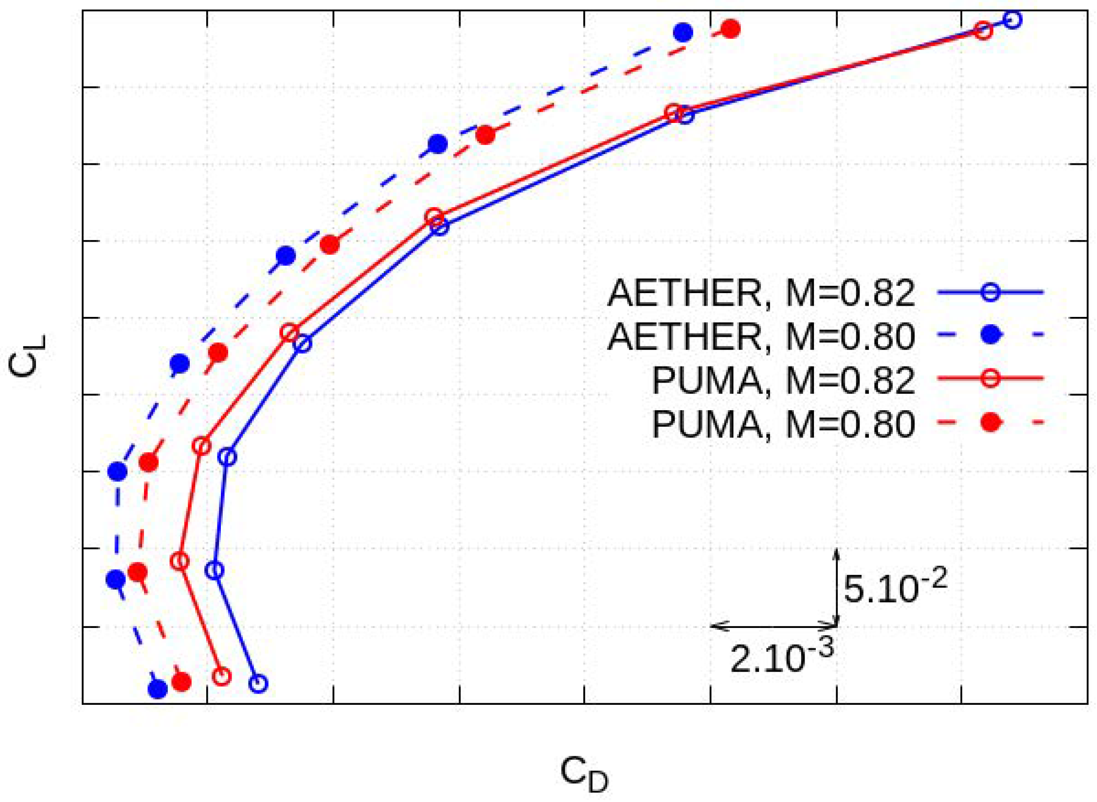
2.4. Aerodynamic Cross Comparisons
3. Aerostructural Optimization Tools
3.1. Structural Analysis Model
3.2. Jig Shape Computation
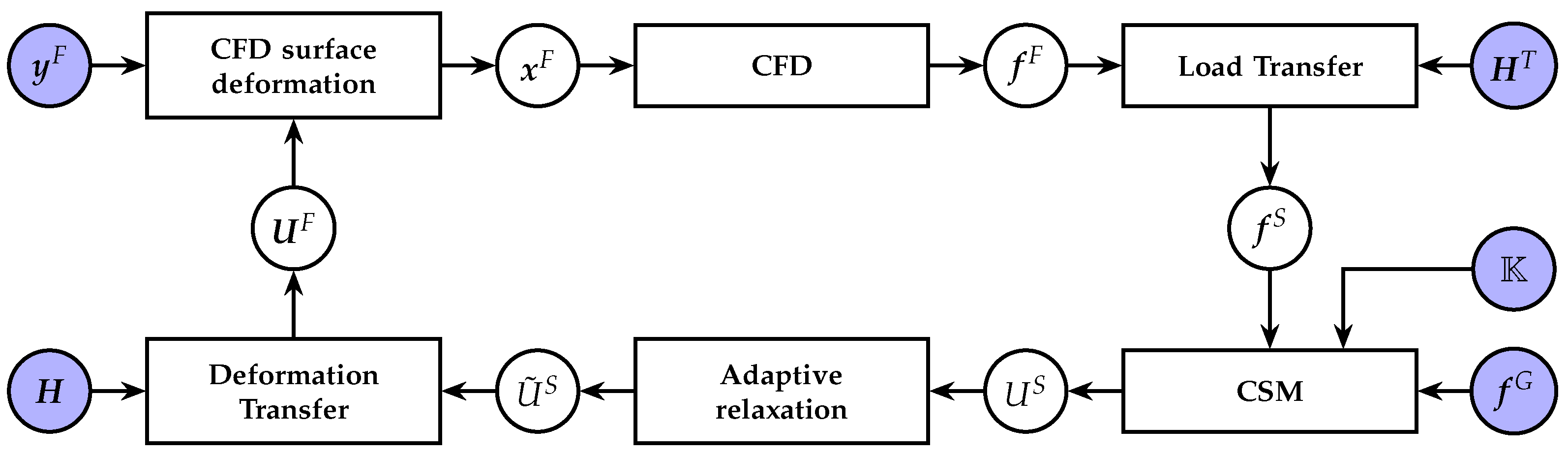
3.3. Coupled Flow and Structural Analysis Tool
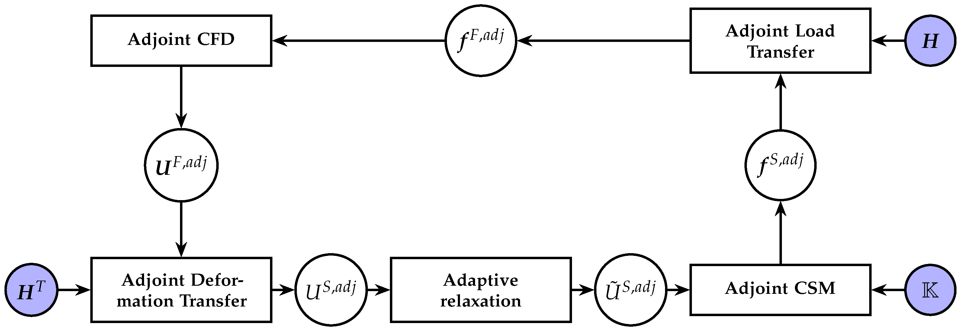
3.4. Coupled Adjoint Flow and Structural Solver
4. Applications
4.1. Aerodynamic Shape Optimization with Rigid Wing Structure
4.2. Aerostructural Shape Optimization
4.2.1. Single-Point Optimization with Fixed Structural Model
4.2.2. Two-Point Optimization with Fixed Structural Model
4.2.3. Optimization with Varying Structural Model
5. Discussion and Conclusions
Author Contributions
Funding
Institutional Review Board Statement
Informed Consent Statement
Data Availability Statement
Acknowledgments
Conflicts of Interest
Abbreviations
| CFD | Computational Fluid Dynamics |
| CSM | Computational Structural Mechanics |
| FDs | Finite Differences |
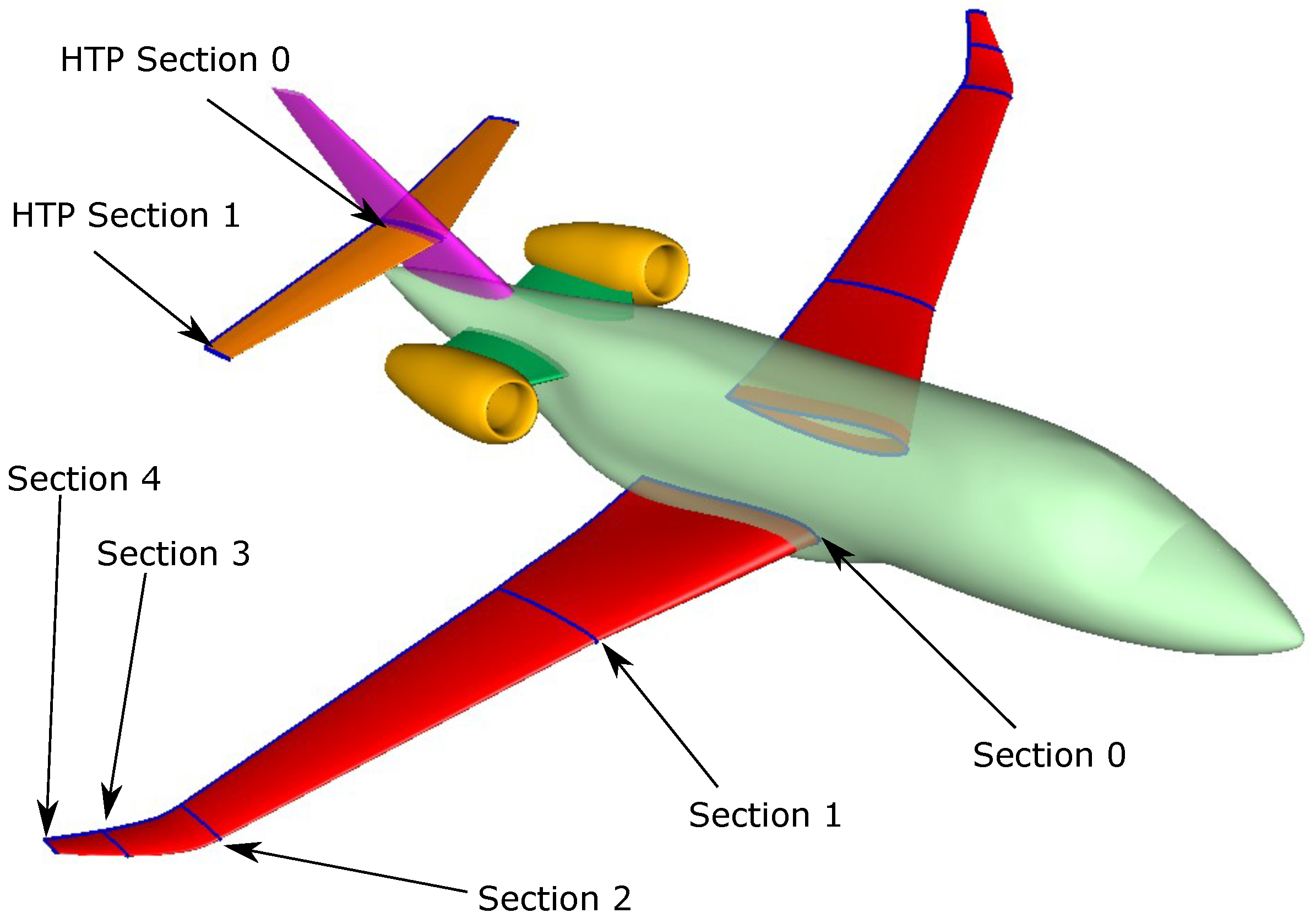
| GBJ | Generic Business Jet |
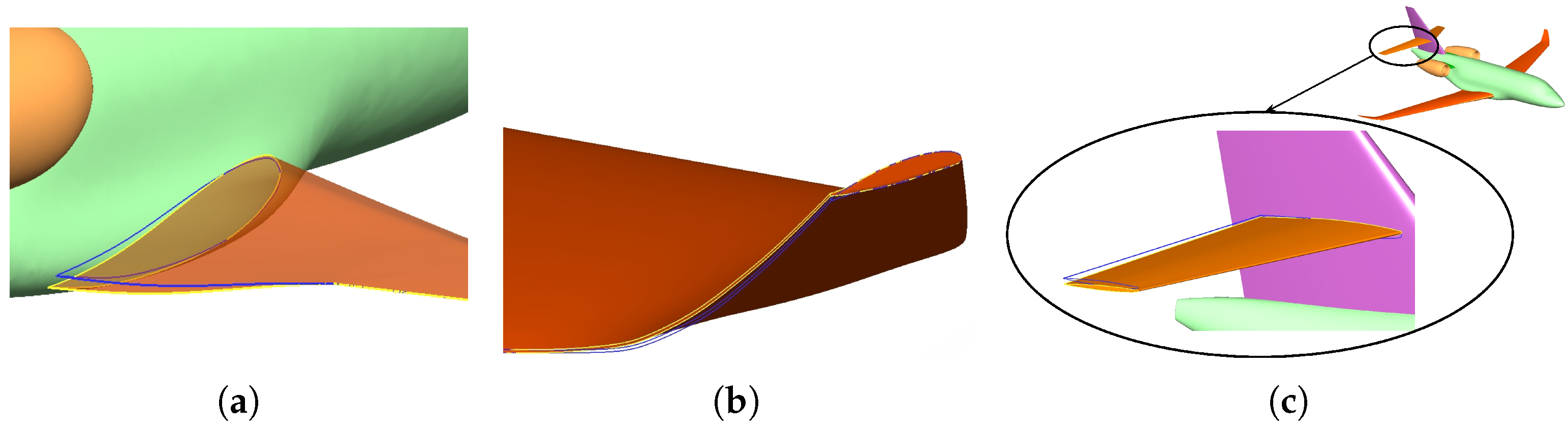
| HTP | Horizontal Tail Plane |
| MDO | Multi-Disciplinary Optimization |
| RANS | Reynolds-Averaged Navier-Stokes |
| RBF | Radial Basis Function |
| SM | Surrogate Model |
| SDs | Sensitivity Derivatives |
References
- European Commission. Flightpath 2050—Europe’s Vision for Aviation; European Commission: Brusssels, Belgium, 2011. [Google Scholar]
- van der Sman, E.; Peerlings, B.; Kos, J.; Lieshout, R.; Boonekamp, T. Destination 2050—A route to net zero European aviation. NLR-CR-2020-510, 2020. Available online: https://www.destination2050.eu/wp-content/uploads/2021/03/Destination2050_Report.pdf (accessed on 2 February 2024).
- Dwight, R.; Brezillon, J. Effect of approximations of the discrete adjoint on gradient-based optimization. AIAA J. 2006, 44, 3022–3031. [Google Scholar] [CrossRef]
- Kim, C.; Kim, C.; Rho, O. Feasibility study of constant eddy-viscosity assumption in gradient-based design optimization. J. Aircr. 2003, 40, 1168–1176. [Google Scholar] [CrossRef]
- Martin, L.; Forestier, N.; Colo, L.; Billard, F.; Chalot, F.; Johan, Z.; Mallet, M. Extension of Linearized CFD Methods for Complex Aerodynamic Flows and Application to Unsteady Load Evaluations. In Proceedings of the International Forum on Aerolasticity and Structural Dynamics, IFASD 2022, Madrid, Spain, 13–17 June 2022. [Google Scholar]
- Zymaris, A.; Papadimitriou, D.; Giannakoglou, K.; Othmer, C. Continuous Adjoint Approach to the Spalart-Allmaras Turbulence Model for Incompressible Flows. Comput. Fluids 2009, 38, 1528–1538. [Google Scholar] [CrossRef]
- Bueno-Orovio, A.; Castro, C.; Palacios, F.; Zuazua, E. Continuous adjoint approach for the Spalart-Allmaras model in aerodynamic optimization. AIAA J. 2012, 50, 631–646. [Google Scholar] [CrossRef]
- Haftka, R. Optimization of flexible wing structures subject to strength and induced drag constraints. AIAA J. 1977, 15, 1101–1106. [Google Scholar] [CrossRef]
- Sobieszczanski-Sobieski, J. Structural Shape Optimization in Multidisciplinary System Synthesis; NASA Technical Memorandum 100538; Springer: Dordrecht, The Netherlands, 1988. [Google Scholar]
- Martins, J.R.R.A.; Alonso, J.; Reuther, J. High-Fidelity Aerostructural Design Optimization of a Supersonic Business Jet. J. Aircr. 2004, 41, 523–530. [Google Scholar] [CrossRef]
- Kenway, G.K.W.; Kennedy, G.J.; Martins, J.R.R.A. Scalable Parallel Approach for High-Fidelity Steady-State Aeroelastic Analysis and Adjoint Derivative Computations. J. Comput. Phys. 2014, 52, 935–951. [Google Scholar] [CrossRef]
- Abu-Zurayk, M.; Brezillon, J. Shape Optimization Using the Aero-structural Coupled Adjoint Approach for Viscous Flows. In Proceedings of the EUROGEN 2011, Capua, Italy, 14–16 September 2011. [Google Scholar]
- Ghazlane, I.; Carrier, G.; Dumont, A.; Desideri, J.A. Aerostructural Adjoint Method for Flexible Wing Optimization. In Proceedings of the 53rd AIAA/ASME/ASCE/AHS/ASC Structures, Structural Dynamics and Materials Conference, Honolulu, HI, USA, 23–26 April 2012. [Google Scholar]
- Merle, A.; Ilic, C.; Abu-Zurayk, M.; Häßy, J.; Becker, R.; Schulze, M.; Klimmek, T. High-Fidelity Adjoint-based Aircraft Shape Optimization with Aeroelastic Trimming and Engine Coupling. In Proceedings of the EUROGEN 2019, Guimarães, Portugal, 12–14 September 2019. [Google Scholar]
- Abu-Zurayk, M.; Merle, A.; Ilic, C.; Keye, S.; Goertz, S.; Schulze, M.; Klimmek, T.; Kaiser, C.; Quero, D.; Häßy, J.; et al. Sensitivity-based Multifidelity Multidisciplinary Optimization of a Powered Aircraft Subject to a Comprehensive Set of Loads. In Proceedings of the AIAA AVIATION 2020 Forum, Virtual Event, 15–19 June 2020. [Google Scholar]
- Bombardieri, R.; Cavallaro, R.; Sanchez, R.; Gauger, N. Aerostructural wing shape optimization assisted by algorithmic differentiation. Struct. Multidiscip. Optim. 2021, 64, 739–760. [Google Scholar] [CrossRef]
- Bons, N.; Martins, J.R.R.A. Aerostructural Design Exploration of a Wing in Transonic Flow. Aerospace 2020, 7, 118. [Google Scholar] [CrossRef]
- Brooks, T.R.; Martins, J.R.R.A.; Kennedy, G.J. High-fidelity aerostructural optimization of tow-steered composite wings. J. Fluids Struct. 2019, 88, 122–147. [Google Scholar] [CrossRef]
- Coder, J.G.; Pulliam, T.H.; Hue, D.; Kenway, G.K.W.; Sclafani, A.J. Contributions to the 6th AIAA CFD Drag Prediction Workshop Using Structured Grid Methods. In AIAA SciTech Forum; American Institute of Aeronautics and Astronautics: Reston, VA, USA, 2017. [Google Scholar]
- Chalot, F.; Mallet, M.; Ravachol, M. A comprehensive finite element Navier-Stokes solver for low- and high-speed aircraft design. In 32nd Aerospace Sciences Meeting and Exhibit, AIAA 94-0814; American Institute of Aeronautics and Astronautics: Reston, VA, USA, 1994. [Google Scholar]
- Trompoukis, X.; Tsiakas, K.; Asouti, V.; Kontou, M.; Giannakoglou, K. Optimization of an Internally Cooled Turbine Blade—Mathematical Development and Application. Int. J. Turbomach. Propuls. Power 2021, 6, 20. [Google Scholar] [CrossRef]
- ESI-Group. Available online: https://www.esi-group.com/products/virtual-performance-solution/ (accessed on 1 February 2024).
- Kleinveld, S.; Rogé, G.; Daumas, L.; Dinh, Q. Differentiated parametric CAD used within the context of automatic aerodynamic design optimization. In Proceedings of the 12th AIAA/ISSMO Multidisciplinary Analysis and Optimization Conference, Victoria, BC, Canada, 10–12 September 2008. [Google Scholar]
- Gagliardi, F.; Giannakoglou, K. A Two-Step Radial Basis Function-Based CFD Mesh Displacement Tool. Adv. Eng. Softw. 2019, 128, 86–97. [Google Scholar] [CrossRef]
- Fong, W.; Darve, E. The black-box fast multipole method. J. Comput. Phys. 2009, 228, 8712–8725. [Google Scholar] [CrossRef]
- Hughes, T.; Franca, L.; Mallet, M. A New Finite Element Formulation for Computational Fluid Dynamics: I. Symmetric Forms of the Compressible Euler and Navier-Stokes Equations and the Second Law of Thermodynamics. Comput. Methods Appl. Mech. Eng. 1986, 54, 223–234. [Google Scholar] [CrossRef]
- Chalot, F. Industrial Aerodynamics; John Wiley & Sons: Hoboken, NJ, USA, 2004. [Google Scholar]
- Spalart, P.; Allmaras, S. A one-equation turbulence model for aerodynamic flows. Rech. Aérospatiale 1992, 1, 5–21. [Google Scholar]
- Saad, Y.; Schultz, M.H. GMRES: A Generalized Minimal Residual Algorithm for Solving Nonsymmetric Linear Systems. SISC 1986, 7, 856–869. [Google Scholar] [CrossRef]
- Martin, L.; Rogé, G. Calcul de la sensibilité d’ordre deux d’une observation aérodynamique. ESAIM Procs 2009, 27, 138–155. [Google Scholar] [CrossRef]
- Hascoët, L. TAPENADE: A Tool for Automatic Differentiation of programs. In Proceedings of the 4th European Congress on Computational Methods in Applied Sciences and Engineering (ECCOMAS), Jyvaskyla, Finland, 24–28 July 2004. [Google Scholar]
- Shroff, G.; Herbert, B. Stabilization of unstable procedures: The Recursive Projection Method. SIAM J. Numer. Anal. 1993, 40, 1099–1120. [Google Scholar] [CrossRef]
- Brooks, T.R.; Kenway, G.J.; Martins, J.R.R.A. Benchmark Aerostructural Models for the Study of Transonic Aircraft Wings. AIAA J. 2018, 56, 2840–2855. [Google Scholar] [CrossRef]
- European Aviation Safety Agency. Available online: https://www.easa.europa.eu/en/certification-specifications/cs-25-large-aeroplanes (accessed on 13 January 2024).
- Jakobsson, S.; Amoignon, O. Mesh deformation using Radial Basis Functions for gradient-based aerodynamic shape optimization. Comput. Fluids 2007, 36, 1119–1136. [Google Scholar] [CrossRef]
- Farhat, C.; Lesoinne, M.; LeTallec, P. Load and motion transfer algorithms for fluid/structure interaction problems with non-matching discrete interfaces: Momentum and energy conservation, optimal discretization and application to aeroelasticity. Comput. Methods Appl. Mech. Eng. 1998, 157, 95–114. [Google Scholar] [CrossRef]
- Degroote, J.; Haelterman, R.; Annerel, S.; Bruggeman, P.; Vierendeels, J. Performance of partitioned procedures in fluid-structure interaction. Comput. Struct. 2010, 88, 446–457. [Google Scholar] [CrossRef]
- Kraft, D. Algorithm 733: TOMP–Fortran modules for optimal control calculations. ACM Trans. Math. Softw. 1994, 20, 262–281. [Google Scholar] [CrossRef]


| to | |||
| to | |||
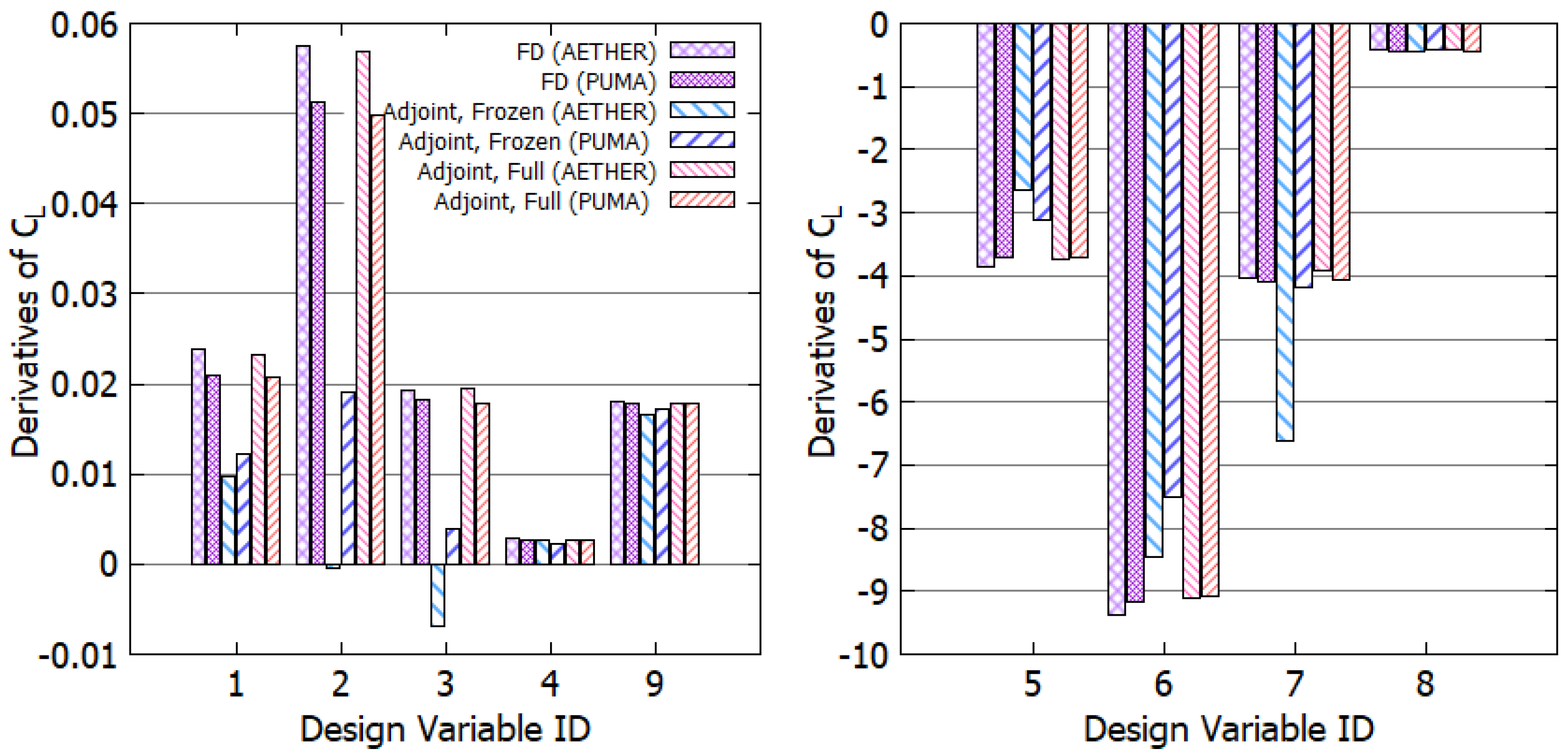
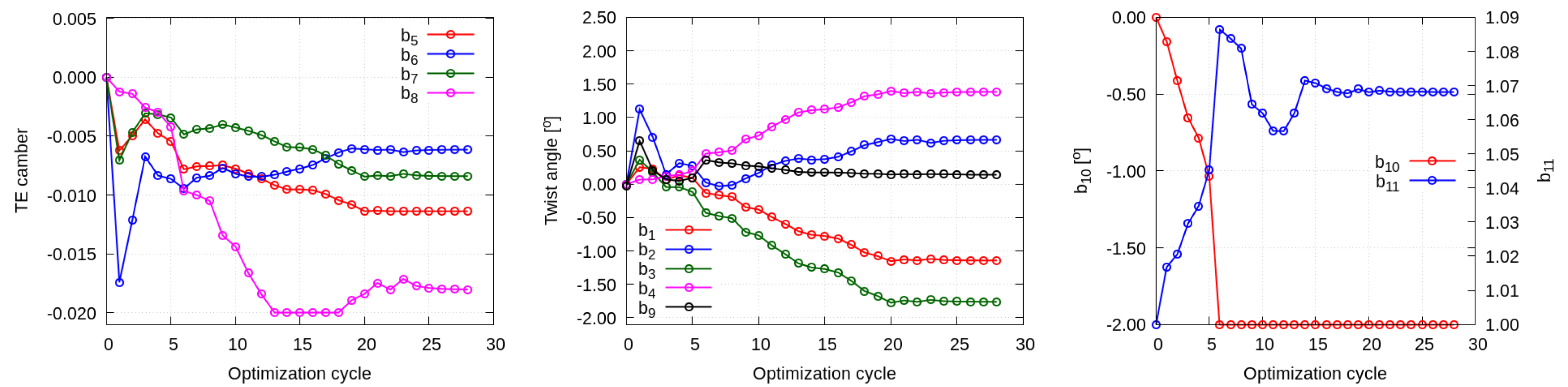
| Var ID | |||||||||
|---|---|---|---|---|---|---|---|---|---|
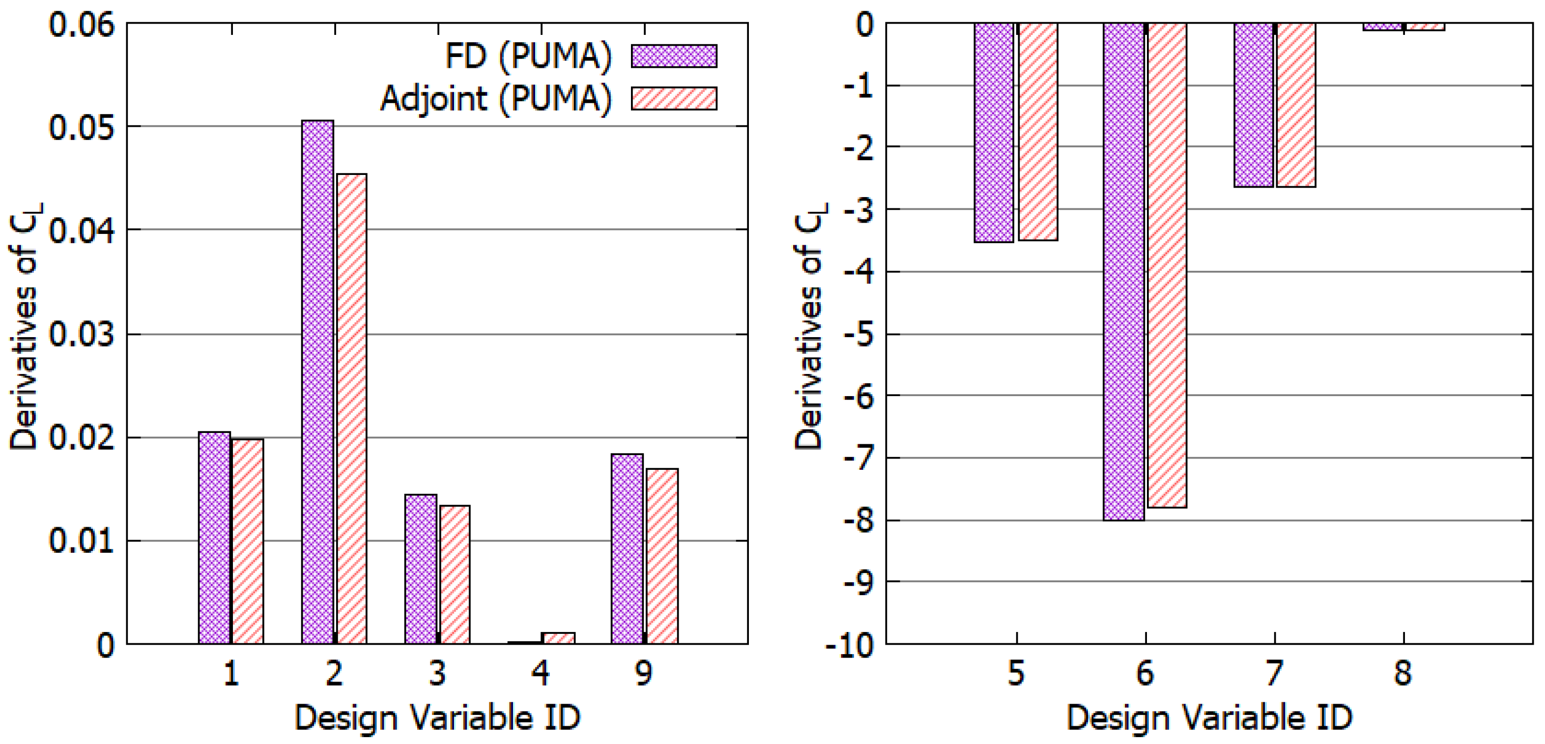
| AETHER | −1.579 | 1.290 | 0.409 | 0.454 | −0.00208 | 0.00422 | 0.00506 | −0.0176 | −0.0374 |
| PUMA | −2.000 | 1.129 | 0.318 | 0.178 | −0.00645 | 0.00375 | 0.00446 | −0.0171 | −0.1752 |
Disclaimer/Publisher’s Note: The statements, opinions and data contained in all publications are solely those of the individual author(s) and contributor(s) and not of MDPI and/or the editor(s). MDPI and/or the editor(s) disclaim responsibility for any injury to people or property resulting from any ideas, methods, instructions or products referred to in the content. |
© 2024 by the authors. Licensee MDPI, Basel, Switzerland. This article is an open access article distributed under the terms and conditions of the Creative Commons Attribution (CC BY) license (https://creativecommons.org/licenses/by/4.0/).
Share and Cite
Tsiakas, K.; Trompoukis, X.; Asouti, V.; Giannakoglou, K.; Rogé, G.; Julisson, S.; Martin, L.; Kleinveld, S. Discrete and Continuous Adjoint-Based Aerostructural Wing Shape Optimization of a Business Jet. Fluids 2024, 9, 87. https://doi.org/10.3390/fluids9040087
Tsiakas K, Trompoukis X, Asouti V, Giannakoglou K, Rogé G, Julisson S, Martin L, Kleinveld S. Discrete and Continuous Adjoint-Based Aerostructural Wing Shape Optimization of a Business Jet. Fluids. 2024; 9(4):87. https://doi.org/10.3390/fluids9040087
Chicago/Turabian StyleTsiakas, Konstantinos, Xenofon Trompoukis, Varvara Asouti, Kyriakos Giannakoglou, Gilbert Rogé, Sarah Julisson, Ludovic Martin, and Steven Kleinveld. 2024. "Discrete and Continuous Adjoint-Based Aerostructural Wing Shape Optimization of a Business Jet" Fluids 9, no. 4: 87. https://doi.org/10.3390/fluids9040087
APA StyleTsiakas, K., Trompoukis, X., Asouti, V., Giannakoglou, K., Rogé, G., Julisson, S., Martin, L., & Kleinveld, S. (2024). Discrete and Continuous Adjoint-Based Aerostructural Wing Shape Optimization of a Business Jet. Fluids, 9(4), 87. https://doi.org/10.3390/fluids9040087