In this section, results are presented with a specific focus on the flow above and close to the permeable wall. Some of the relevant turbulent structures are analyzed by first identifying and distinguishing the zones of vortex motion in the permeable boundary layer flow and their dynamical generation. Their order, shape, extent, and orientation are then considered. Subsequently, specific events associated with the motions of these structures are determined. The analysis is then completed with an overview of the dominant energy modes associated with the structures.
4.1. Identification and Distinction of Vortex Regions
The identification of vortex regions has been one of the highlights of previous studies of turbulent flow over permeable boundaries (e.g., ref. [
2]). This is because it provides important information about the size, reach, and motions of organized structures in a turbulent flow. With planar PIV data, one is able to visualize vortices on whole flow field vector maps through decompositional methods such as Galilean, Reynolds, and large-eddy simulation (LES) methods [
22]. Examples of these are shown in
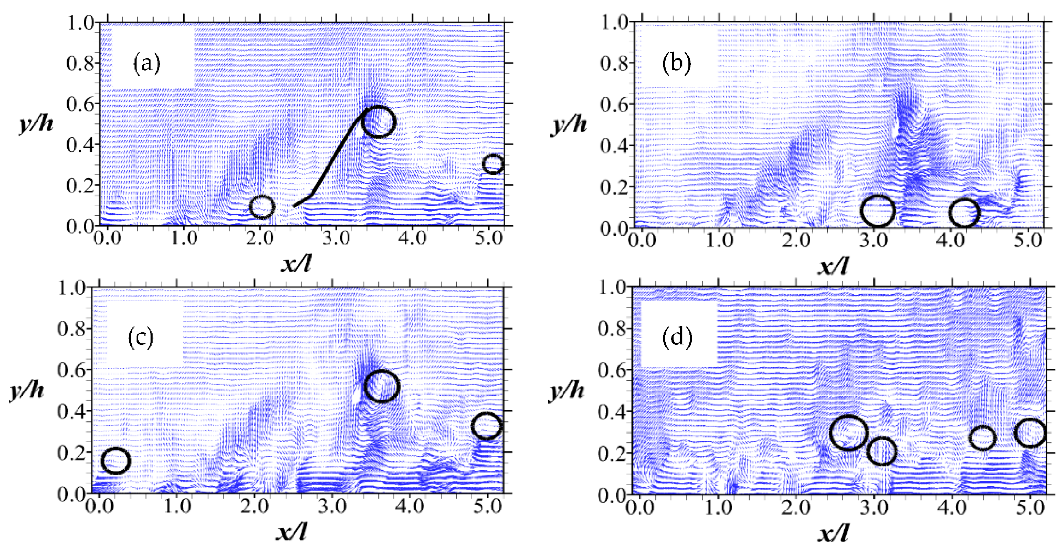
Figure 3. With the Galilean decomposition, large-scale vortex cores are identified. Indeed, there are few indicators of hairpin vortices close to the permeable wall. This is shown in
Figure 3a, where features such as the vortex head, inclined areas of ejection vectors, stagnation points, and inclined shear layer [
29] are apparent. The small-scale vortices are more evident using the Reynolds decomposition and LES method. In
Figure 3a–c, these features are compared for the same measurement taken at the same instant during Test A. Another sample Galilean decomposition is presented for Test B data in
Figure 3d. Overall, these maps display a wide range of vortex cores, apparently within a wall-normal height of 60% of the porous medium depth
h.A more common criterion for vortex identification, however, is the vorticity parameter. By using that criterion in
Figure 4, a complex but organized system of vortex cores of mean spanwise vorticities (Ω
z = ∂
V/∂x − ∂
U/∂y) is shown. These cores are positioned close to the permeable boundary. While there are isolated small regions of intense positive vorticities, the negative vorticities are more widespread and bigger. The reason why these regions have negative vorticities is that those regions have a relatively small mean wall-normal velocity gradient in the streamwise coordinate (∂
V/∂x) compared with the mean streamwise velocity gradient in the wall-normal direction (∂
U/∂y). It is also noted that the intensities of the vorticities appear to decline downstream. This is consistent with observations in a previous study regarding the dissipation of vorticity downstream of the compact porous medium [
12].
The locations and sizes of these vortex cores are dependent on the Reynolds number and streamwise locations with respect to the porous boundary. In terms of the locations, for example, the vortex cores of Test A are generally found just above the porous medium rods. Consequently, they also tend to rise above the boundary, up to a height of 0.40 h. The vorticities of Test B, on the other hand, perhaps being freer to communicate with the porous medium through the pore spacing, are found in between the rods. Thus they barely rise beyond a magnitude of 0.30 h, except for the rare case of a peak vortex. It is also clear that while the streamwise extent of the vortex cores is 60% or less of the distance between the rods for the first six columns of rods, they are more extensive downstream. It appears that due to the compactness of the porous medium, the vortex cores have a downward inclination downstream of the porous medium.
While an important criterion for detecting vortex regions, vorticity maps are not able to distinguish between regions arising from pure rotation and those from shear. Thus, as outlined in
Section 3.1, to show such distinctions of vorticity generation, eigenanalysis of the mean velocity gradient are used to retrieve the shear and swirling strengths. The results of these analyses are shown in
Figure 5 and
Figure 6, respectively, normalized by the maximum entry velocity and the rod diameter. Unsurprisingly, the contour plots in
Figure 5 show that the dynamical generation of the vortex cores of the flow is mostly due to shear. The shear regions appear to extend from within the porous medium itself. For the case of Test A, the shear strength is highest at the very edge of the permeable boundary. This is indicative of the kind of high shear zones that tend to activate Kelvin–Helmholtz instabilities that lead to the formation of spanwise rollers [
2,
12]. It is also noteworthy that these shear regions are elongated and intermitted with thin regions of no shear. While these are certainly not the streaky structures associated with boundary layer flows of impermeable walls [
29], they are reminiscent of them, and more so at higher Reynolds number flows. However, instead of being aligned in the streamwise direction, these ‘streaky’ structures associated with the shear strength are aligned in the wall-normal directions. In
Figure 6, the regions of vorticity emanating from swirls are shown to be sparse and generally detached from the permeable boundary. However, at a higher Reynolds number, rotation becomes a more effective method of generating vorticity. These are the vorticities that peak off at a relatively higher wall-normal location compared to the others.
4.2. Special Features of Spatial Structures
In order to investigate the order, shape, extent, and orientation of the coherent structures in further detail, two-point spatial autocorrelation functions of the streamwise fluctuating velocities (
Ruu) and the wall-normal fluctuating velocities (
Rvv) are used. The spatial coherence of organized structures of the flow is illustrated using sample iso-contours of the correlation profiles in
Figure 7. For those plots, the contours are centered at (
x/l = 0,
y/h = 0.54), and (
x/l = 11,
y/h = 0.54) for both Tests A and B. The contour levels for each of the plots are 0.5, 0.6, 0.7, 0.8, and 0.9, respectively, in an inward direction towards the core of the contour. These results pertain to extreme streamwise locations immediately above the rods of the permeable boundary and within the midspan plane. Thus, they provide a satisfactory preliminary insight into the evolution of organized structures across the permeable boundary layer turbulent flow.
It is evident that the
Ruu contours are larger and more elongated in shape along the stream than in the wall-normal direction. There is also a quasi-streamwise alignment of the contours. These features are particularly so around the most upstream column of rods of the permeable boundary and less so at the most downstream rod locations. The extent and elongation of
Ruu contours point to the existence of spatial structures of the flow that are more organized in the streamwise direction relative to the wall-normal direction. Compared with
Ruu, the
Rvv contours are more condensed and rounded. Overall, some of these observations are similar to those reported elsewhere for channel flows over smooth and rough impermeable walls [
30].
Following the methodology outlined in previous works [
30,
31], a more comprehensive assessment of the evolution of the average size and inclination of the correlation function contours is conducted. This is performed on the basis that such an assessment will provide an indication of the extent, shape, and orientation of structures such as hairpin vortices associated with turbulent boundary layers [
24]. In order to study the wall-normal changes in size and inclinations associated with the autocorrelation functions, contours of
Ruu and
Rvv were obtained for different wall-normal positions (ranging from
y/h = 0.04 to 1.54) per two fixed streamwise locations (at
x/l = 0 and 11 respectively). The streamwise variations were studied by examining the contours of
Ruu and
Rvv retrieved from various streamwise locations (
x/l = 0.10 to 11.80), for which the wall-normal location is fixed at
y/h = 0.243 (i.e., close to the permeable boundary).
In order to estimate the relative contour sizes, the streamwise and wall-normal spatial extents of
Rvv (signified by
Lxvv and by
Lyvv, respectively) were correspondingly evaluated as the streamwise and wall-normal distances between the extreme points on the
Rvv = 0.5 contour level. For the
Ruu contours, the streamwise extent of
Ruu (signified by
Lxuu) was evaluated as twice the distance between the most downstream point on the
Ruu = 0.5 contour level and the self-correlation peak. The wall-normal extent of
Ruu (signified by
Lyuu) was also evaluated as the wall-normal distance between the furthest and closest locations from the permeable boundary on the
Ruu = 0.5 contour level. It is noted that these central locations of the contours were selected in a way that assessments are unaffected by the edges of the respective image frames. The results of the wall-normal and streamwise variations of the spatial extents of the contours are respectively presented in
Figure 8 and
Figure 9. In order to magnify wall-normal differences,
Figure 8 is shown as log-linear plots. Approximations of the average angles of streamwise inclination of
Ruu (i.e.,
β in degrees) were also made as described in
Section 3.2. The results are shown in
Figure 10.
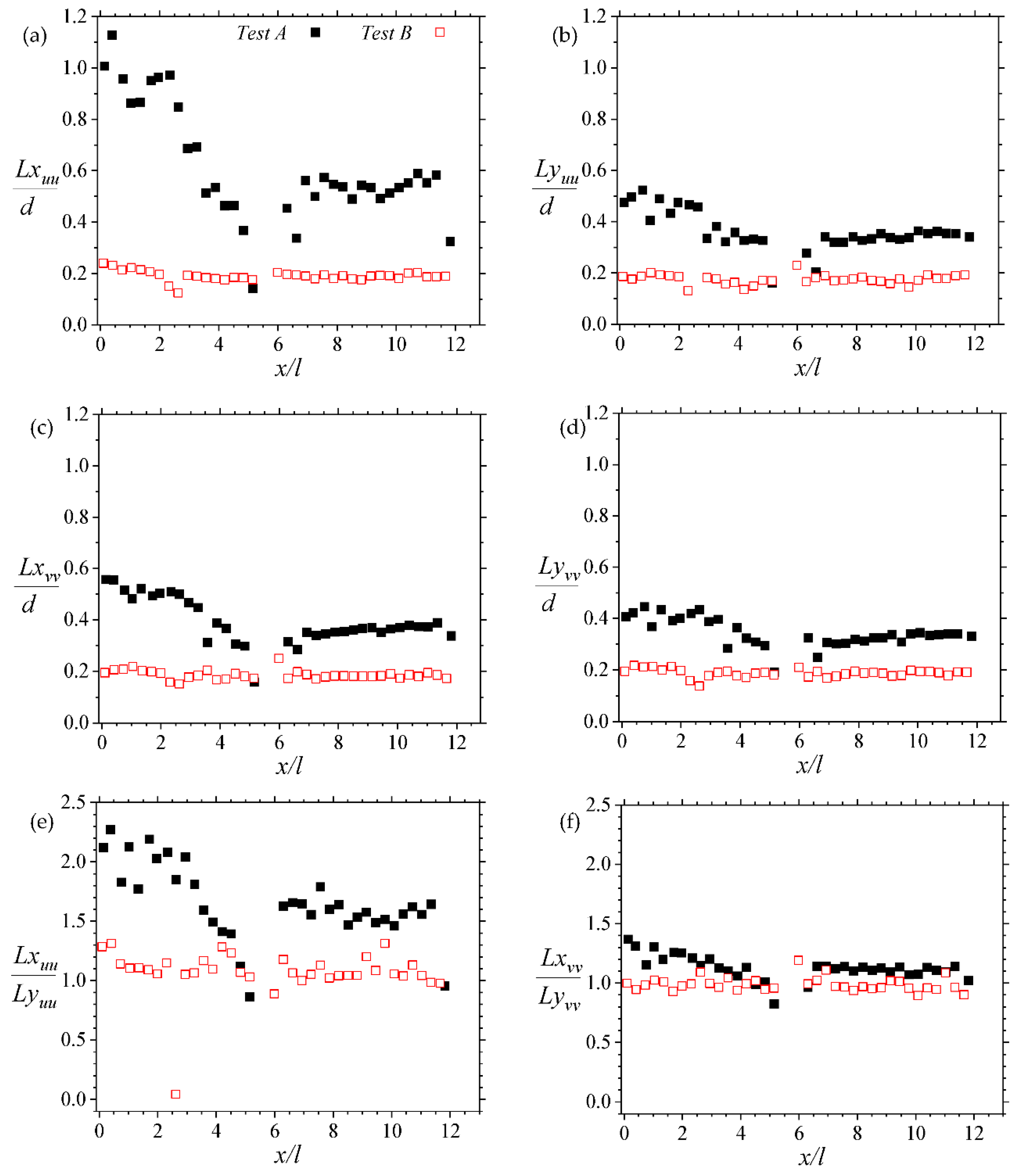
In general, the data in
Figure 8 confirm the observations qualitatively deduced from
Figure 7. However, additional details are apparent. Firstly, the trend in wall-normal variations of the streamwise and wall-normal spatial extents of the correlation functions are similar at the downstream and upstream locations of the permeable boundary. Just above the boundary, the spatial extents are usually less than 10% of the diameter
d of the porous medium rods. However, the sizes tend to increase initially with the wall-normal location. The sizes then dip slightly after peaking off (for Test A), or they plateau at 1.5
h (for Test B). The initial increment in extent is Reynolds number dependent. While that of Test B (the higher Reynolds number test) is marginal, Test A (the lower Reynolds number test) is up to three times the corresponding value of Test A. Notwithstanding this difference, the general increase implies that further away from the permeable boundary, the flow’s spatial structures tend to be more correlated. Indeed, it appears that this wall-normal correlation is much better at the leading edge of the porous boundary than at the trailing edge.
Additionally, as presented in
Figure 8, the ratios of the streamwise to wall-normal extents for
Ruu, are, on average, 1.8 and 1.4 at
x/l = 0 and 11. For
Rvv, the ratios of the extents are closer to 1. While the ratios for
Ruu are less than what has been reported for turbulent flows over smooth walls or rough walls, that of
Rvv are comparable with those reported for both kinds of near-wall boundary layer flows [
32].
Figure 8.
Log-linear plots showing wall-normal variations of the streamwise and wall-normal extents of the two-point correlations (2PC) at two streamwise locations above the porous boundary. Note that Lxuu, Lyuu, Lxvv, Lyvv are respectively the streamwise extent of the 2PC of the streamwise velocity, wall-normal extent of the 2PC of the streamwise velocity, streamwise extent of the 2PC of the wall-normal velocity, wall-normal extent of the 2PC of the wall-normal velocity. Legend in (a) applies to all plots in (b–f).
From
Figure 9, it may also be inferred that for Test B, the spatial extents of the correlation function contours and their streamwise/wall-normal ratios are independent of the streamwise location. Thus, the spatial structures are not expected to grow along the stream over a compact porous medium at such high Reynolds numbers. However, at much lower Reynolds numbers, such as in Test A, the spatial extents reduce dramatically along the stream to a minimum at approximately
x/l = 5. Subsequently, their values become constant further downstream. The reason for this initial sharp decline is unclear. Nevertheless, these observations are consistent with vortex zone markers apparent in the vector maps that were previously reviewed.
Figure 9.
Linear plots showing streamwise variations of the streamwise and wall-normal extents of the two-point correlations (2PC) for Tests A and B. Note that Lxuu, Lyuu, Lxvv, Lyvv are respectively the streamwise extent of the 2PC of the streamwise velocity, wall-normal extent of the 2PC of the streamwise velocity, streamwise extent of the 2PC of the wall-normal velocity, wall-normal extent of the 2PC of the wall-normal velocity. Legend in (a) applies to all plots in (b–f).
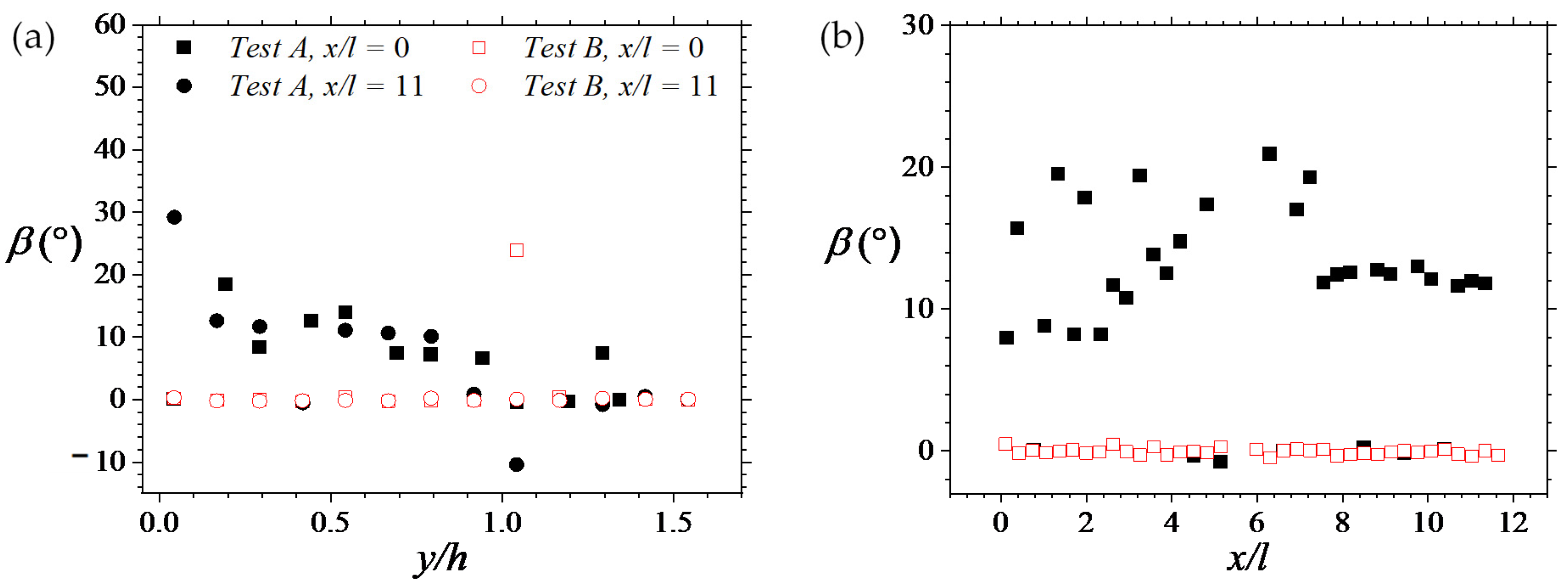
The results of the assessed angles of inclination are shown in
Figure 10. They show that for Test A, the angles decay with the increase in wall-normal distance from the permeable boundary. Along the stream, the angles of streamwise inclination show significant scatter ranging from 0 to ~25
for the first six columns of porous medium rods and then become fairly constant at around 10
. For Test B, on the other hand, the flow behavior is quite different. The correlation function contours are essentially aligned perfectly in the streamwise direction.
If the angle of inclination of
Ruu is taken as the average inclination of the hairpin packets [
31], then those spatial structures are expected to be inclined, as shown in
Figure 10. It is important to note, however, that the angles estimated here are much broader than the range (i.e., 15 ± 5
) reported for canonical turbulent flows [
30,
33,
34,
35].
Figure 10.
(a)Wall-normal variation and (b) Streamwise variation of the angle of streamwise inclination of the two-point correlation of the streamwise velocities. Note that for (b), filled boxes represent Test A results whereas red unfilled boxes are for Test B.
Figure 10.
(a)Wall-normal variation and (b) Streamwise variation of the angle of streamwise inclination of the two-point correlation of the streamwise velocities. Note that for (b), filled boxes represent Test A results whereas red unfilled boxes are for Test B.
4.3. Events of Turbulent Motion
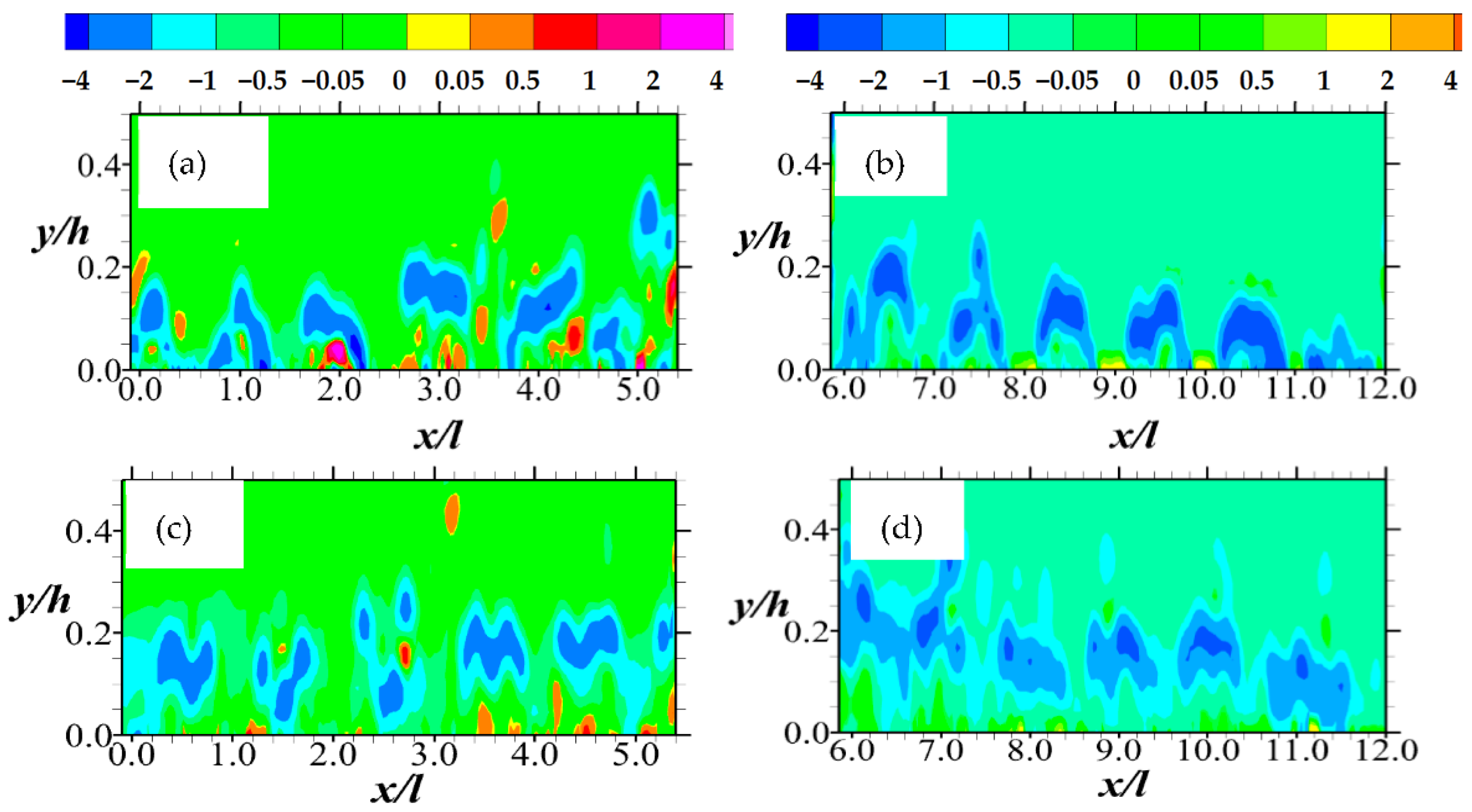
In order to provide some insight into specific events of coherent motions, the information provided through quadrant decomposition is now considered. This analysis serves to specifically characterize the dominant motions associated with the production of Reynolds shear stress. The results are summarily presented through contour plots in
Figure 11,
Figure 12,
Figure 13 and
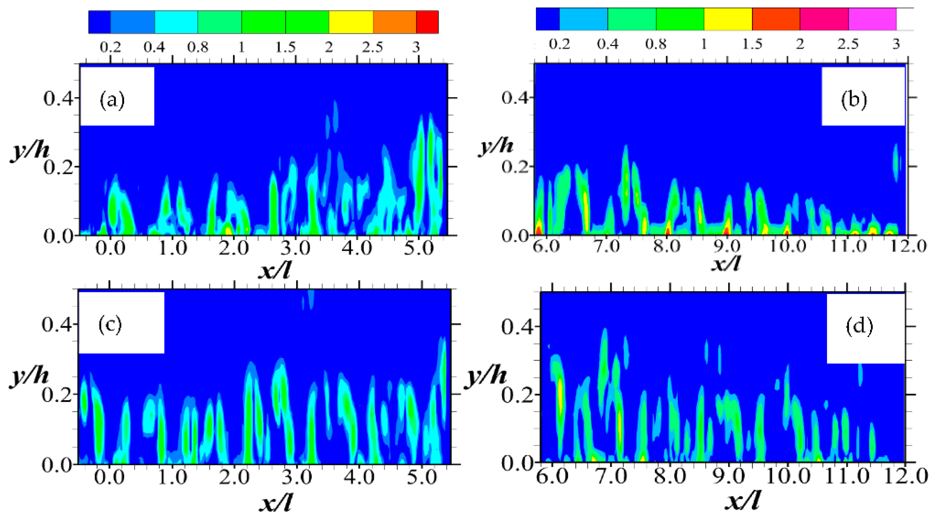
Figure 14. These plots show events of quadrants 1, 3, 2, and 4, respectively, in terms of Reynolds shear stress normalized by the maximum velocity of the entry flow.
As for the spatial features described in
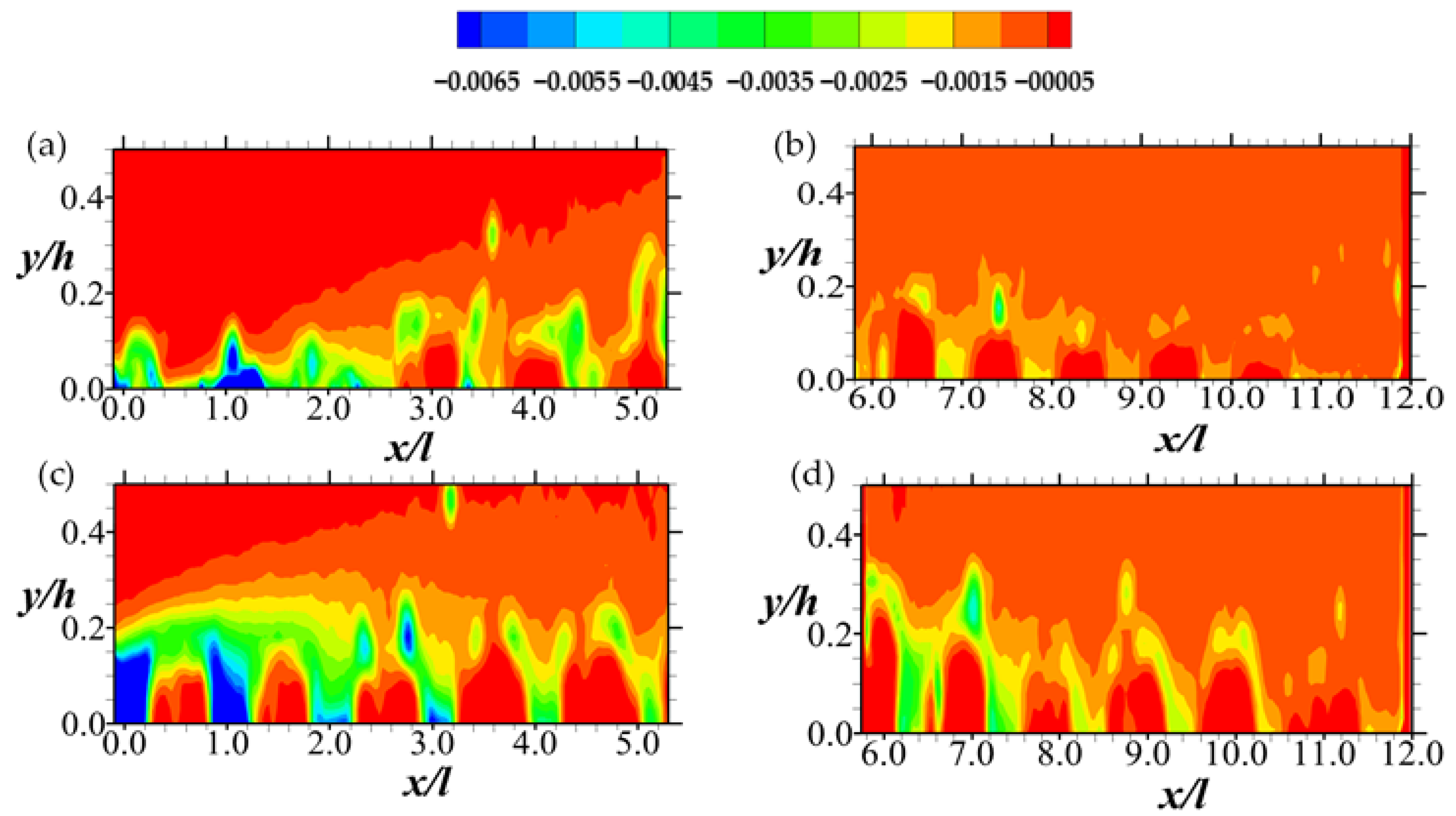
Section 4.2, the results that are shown in this section also indicate that the events of turbulence over the permeable boundary are a function of the Reynolds number as well as the streamwise and wall-normal directions. Thus,
Figure 11 shows that the outward motions of high-speed fluid towards the center of the flow field are somewhat prevalent at the upstream portion (i.e., the first six columns of rods) of the permeable boundary. Further downstream, however, this outward interaction is sedated, particularly for Test A, where the Reynolds number is relatively low. In addition to these streamwise changes in fluid motion, it is important to note that while the outward interaction of the high-speed fluid appears to grow along the stream, particularly around the upstream rods, they subsequently decline. A comparison of
Figure 11 with
Figure 12 shows that apart from the most upstream rows of the permeable boundary rods, the outward interactions of Q1 are much more predominant compared to the inward motion of low-speed fluid of Q3.
Figure 11.
Contour plots of (from Equation (6)) for Quadrant 1 (Q1) events of the Reynolds shear stress normalized by the respective maximum mean streamwise entry velocity. Note that the hole size (i.e., D in Equation (6)) used is 0. The Q1 events are shown in (a,b) for Test A, and (c,d) for Test B. The legend all the plots are above (a,b).
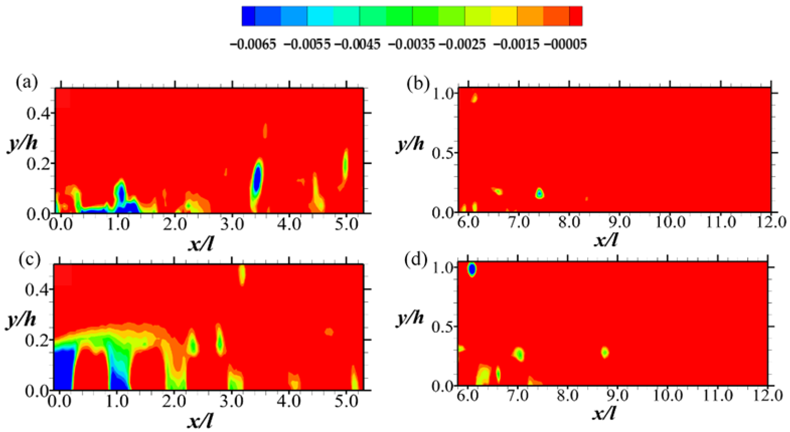
Figure 12.
Contour plots of (from Equation (6)) for Quadrant 3 (Q3) events of the Reynolds shear stress normalized by the respective maximum mean streamwise entry velocity. Note that the hole size (i.e., D in Equation (6)) used is 0. The Q3 events are shown in (a,b) for Test A, and (c,d) for Test B. The legend all the plots are above (a,b).
An examination of
Figure 13 and
Figure 14, on the other hand, indicates that while the intensity of Q1 and Q3 events (i.e., outward and inward interactions) decline downstream, Q2 and Q4 events (i.e., ejections and sweeps, respectively) increase with Q2 dominating slightly. Notably, the results also agree with observations of Suga et al. [
2] that both ejections and sweeps tend to be enhanced close to the permeable boundary. However, it appears that as the Reynolds number increases, the contributions of ejection and sweeps to the shear stress decrease significantly in the downstream region of the porous boundary. These sweep and ejection events are symptomatic of dynamic processes of changes that the structures of turbulence undergo in the permeable boundary layer [
36].
Figure 13.
Contour plots of (from Equation (6)) for Quadrant 2 (Q2) events of the Reynolds shear stress normalized by the respective maximum mean streamwise entry velocity. Note that the hole size (i.e., D in Equation (6)) used is 0. The Q2 events are shown in (a,b) for Test A, and (c,d) for Test B. The legend all the plots are above (a,b).
Figure 14.
Contour plots of (from Equation (6)) for Quadrant 4 (Q4) events of the Reynolds shear stress normalized by the respective maximum mean streamwise entry velocity. Note that the hole size (i.e., D in Equation (6)) used is 0. The Q4 events are shown in (a,b) for Test A, and (c,d) for Test B. The legend all the plots are above (a,b).
It is worth emphasizing that the prevalence of Q1 and Q3 events in the upstream region of the porous boundary is a rather uncommon observation. Even in both impermeable and permeable wall turbulence, it is the dominance of Q2 and Q4 events that are often reported [
2,
4,
5]. Nevertheless, in this case, the observation of significant outward and inward interactions—though rare—explains why negative Reynolds shear stress profiles were observed at the upstream region of the porous boundary in earlier work [
12]. This occurrence is similar to fluid motions that have been reported for a turbulent flow at the leading edge of forward-facing steps [
37] and may perhaps be due to the same physical reasons.
4.4. Characteristics of the Dominant Energy Modes
In this section, the large-scale structures are examined through proper orthogonal decomposition (POD) of the PIV measurements. To this end, the number of snapshots (
N) required to sufficiently capture the energy content for a given mode was determined. This was performed by considering the convergence of fractional energy associated with the most dominant mode (i.e., mode 1) per
N ranging from 10 to 6000. The results are summarized in
Table 2 for both planes of measurement in each Test. As shown, as
N increases, the fractional energy of mode one decreases until a threshold value is attained where the variation is negligible. This threshold value is
N = 4000. In this sample of snapshots, the unchanging values of fractional energy of mode one are 7.8% and (8.65 ± 0.25)% for the data pertaining to planes of measurement in Test A, and 9.3% and 6.8% for those in Test B. Thus,
N = 6000 is more than sufficient to conduct the POD analyses. This number is much higher than what has been reported in a number of related studies [
6,
7].
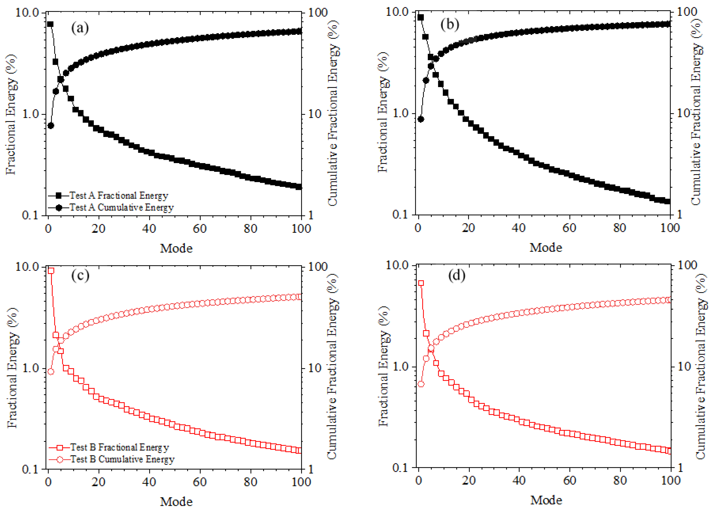
The energy contents of the low-order modes are shown in
Figure 15. This is performed using the spectra of the fractional and cumulative energy contributions of the first 100 modes for the planes of measurement covering the porous boundary condition. The plots indicate an exponential decrease in fractional energy with increasing POD modes. The decay rates are generally greater in the case of Test A relative to Test B. However, the deviation in decay rates between the two tests is greater at 5 <
x/l < 11. To illustrate this, for Test A, 50% of the total energy over the permeable boundary is captured by the first 41 modes and 18 modes at 0 <
x/l < 5 and 5 <
x/l < 11 respectively. For test B, 50% fractional energy is captured by the first 92 and 130 modes at 0 <
x/l < 5 and 5 <
x/l < 11 respectively. Overall, a substantial number of modes (~1550) are required to represent 90% of the fractional energy.
As the first five POD modes have the largest individual values of fractional energy, special attention is focused on them to study the dynamics of the large-scale structures of the flow. Streamwise contours superimposed on vector maps for the eigenmodes are presented in
Figure 16 and
Figure 17 for Tests A and B, respectively. It is important to note that as these are velocity fluctuations of the dominant energy modes, they may be used to reveal regions that correspond to high energy activities of vortices and turbulence events [
38,
39]. Consequently, the results are interpreted using vortex indicators and quadrant definitions (as noted in the figures) to deduce requisite large-scale structures, motions, and events.
Figure 16 indicates that at the highest energy mode, the flow over the permeable boundary at a relatively low Reynolds number is marked by ejections (Q2 events) that are mostly uniform. However, lower energy modes include other motions. At progressively lower-energy modes (e.g., two to four, for instance), the flow is segregated into regions of Q2 and Q4 (sweep) events. Close to alternating regions of Q2 and Q4 events, circulating flow structures are apparent, indicating vortex activity. These Q2 and Q4 events are weaker at lower energy modes. However, they tend to be more in number, along with indicators of vortex activities.
For Test B, the results (shown in
Figure 17) are strikingly different from that of Test A in a number of ways. The most important difference is that Q3 (inward motion of high-speed fluid) and Q1 (outward motion of low-speed fluid) events appear at the upstream section of the permeable boundary at modes one and two. Furthermore, vortex activities are detected as early as mode two. However, it is not until the fourth mode that alternating regions of Q2 and Q4 appear, following the phenomenon in Test A. These POD results essentially confirm observations made in
Section 4.3 about Q1, Q2, Q3, Q4 event markers in the large-scale structural dynamics.
Figure 16.
Streamwise contours and vectors of eigenmodes for Test A. (a,b) are mode 1 with 7.8% and 8.9% fractional energies respectively; (c,d) are mode 2 with 5.8% and 6.8% fractional energies respectively, (e,f) are mode 3 with 3.3% and 5.7% fractional energies respectively; (g,h) are mode 4 with 3.0% and 4.6% fractional energies respectively; (i,j) are mode 5 with 2.2% and 3.6% fractional energies respectively. Legend of the plots are above the plots. Q markers are for quadrant events; VA stands for vortex activity. Scaling of vector magnitudes are not the same for all the plots.
Figure 17.
Contours of eigenmodes for Test B. (a,b) are of mode 1 with 9.3% and 6.8% fractional energies respectively; (c,d) are of mode 2 with 4.1% and 3.2% fractional energies respectively, (e,f) are of mode 3 with 2.1% and 2.1% fractional energies respectively; (g,h) are of mode 4 with 1.9% and 1.8% fractional energies respectively; (i,j) are of mode 5 with 1.5% and 1.5% fractional energies respectively. Legend of the plots are above the plots.


