Hydrodynamic Entrance Length for Laminar Flow in Microchannels with Rectangular Cross Section

Abstract

This work presents a detailed numerical investigation on the required development length ($\mathcal{L}=L/B$) in laminar Newtonian fluid flow in microchannels with rectangular cross section and different aspect ratios ($AR$). The advent of new microfluidic technologies shifted the practical Reynolds numbers ($Re$) to the range of unitary (and even lower) orders of magnitude, i.e., creeping flow conditions. Therefore, accurate estimations of $\mathcal{L}$ at $Re\le \mathcal{O}\left(1\right)$ are important for microsystem design. At such low Reynolds numbers, in which inertial forces are less dominant than viscous forces, flow characteristics become necessarily different from those at the macroscale where $Re$ is typically much larger. A judicious choice of mesh refinement and adequate numerical methods allowed obtaining accurate results and a general correlation for estimating $\mathcal{L}$, valid in the ranges $0\le Re\le 2000$ and $0.1\le AR\le 1$, thus covering applications in both macro and microfluidics.

1. Introduction

Over the past two decades, many microfluidic systems have been designed and built for a wide range of applications. These systems are essentially formed by microchannels and chambers whose geometries have a strong influence on the flow characteristics. Improving the design of such systems requires understanding in detail the fluid flow characteristics. One of the flow characteristics that still needs to be better quantified is the microchannel entrance length, required to achieve fully developed flow, which is an important design parameter especially when it represents a significant fraction of the total microchannel length. However, entrance effects are typically ignored by researchers who usually assume the laminar flow to be fully developed [1].

Different cross-sections (e.g., rectangular, trapezoidal, triangular, circular and elliptical) have been used by numerous researchers with the purpose of exploring the flow behavior in microchannels [2,3,4,5,6,7,8,9]. One important fact that should be highlighted is that the flow field in rectangular channels is more complex than in circular channels, because of the additional dependence on the aspect ratio ($AR$) of the cross-section, as shown in Figure 1.

Figure 1. Schematic representation of the channel geometry. L is the dimensional development length.

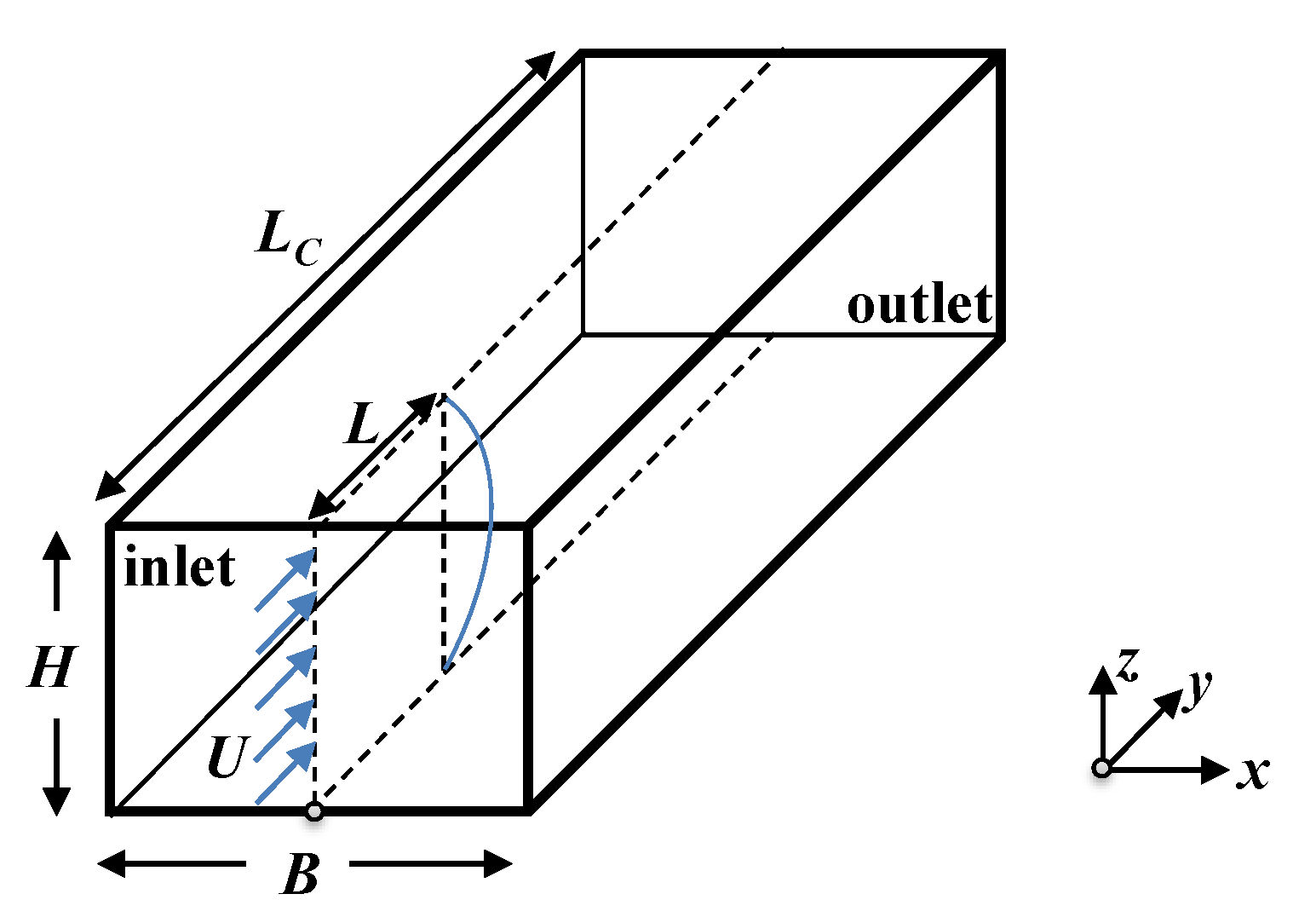
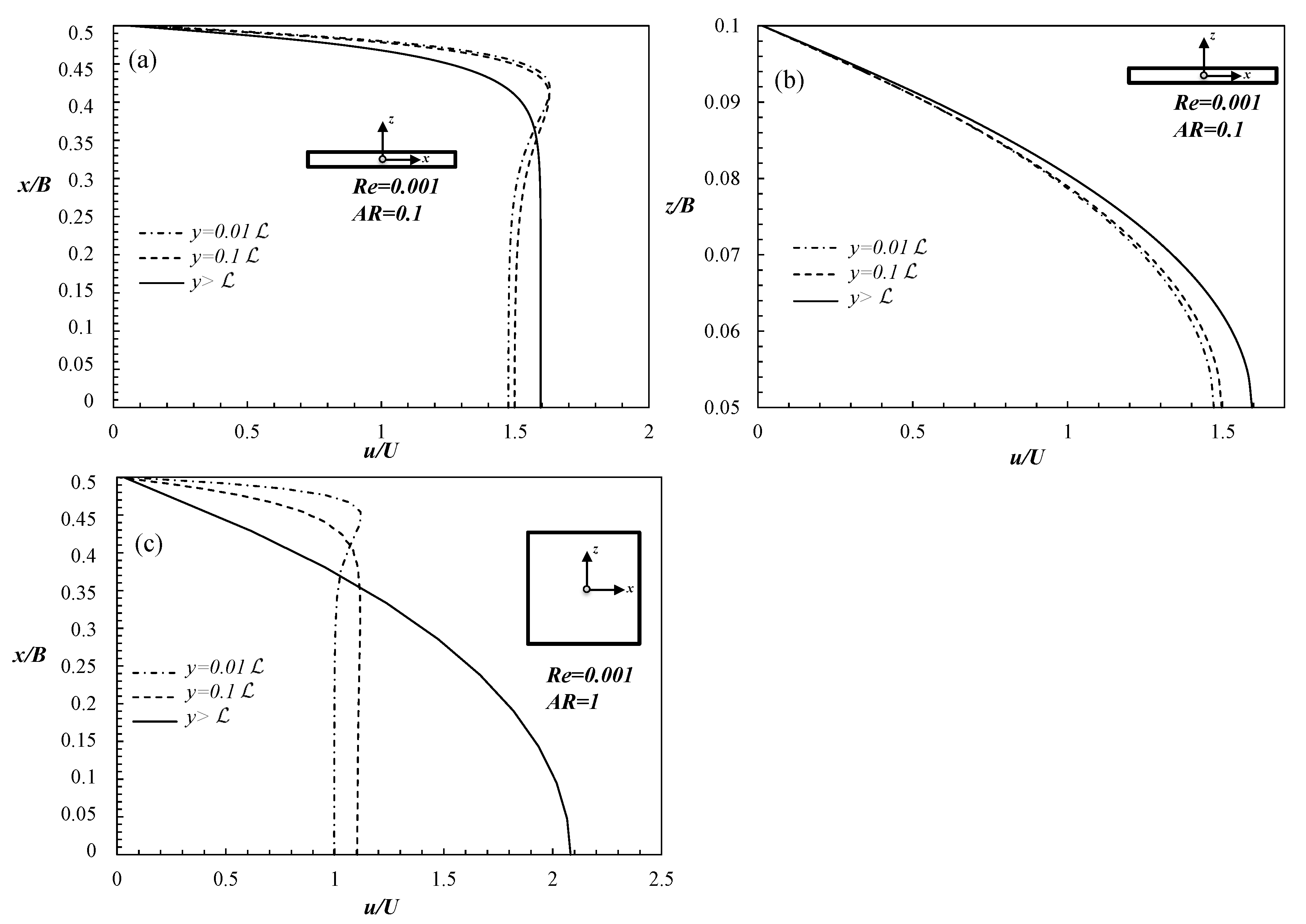
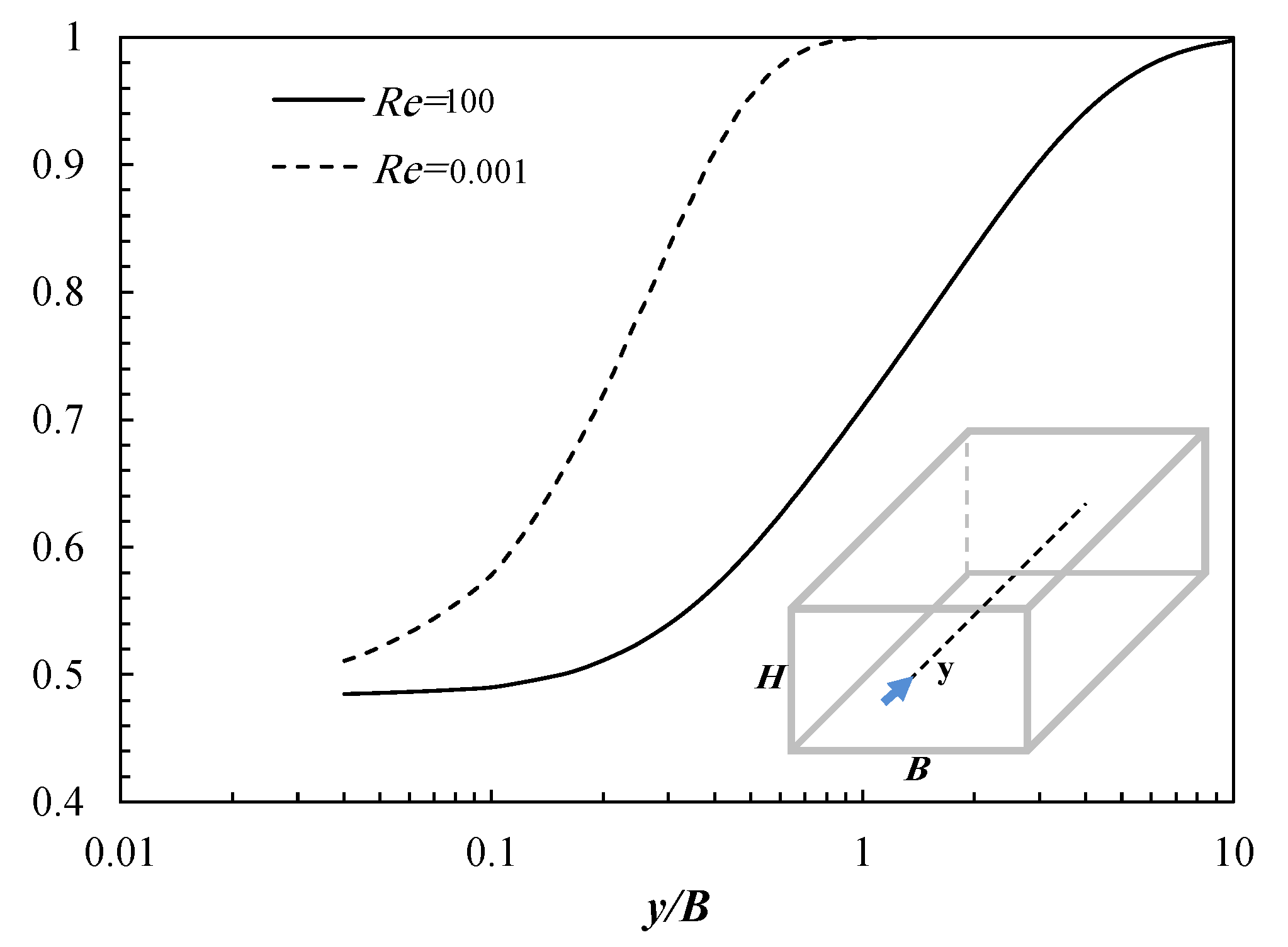
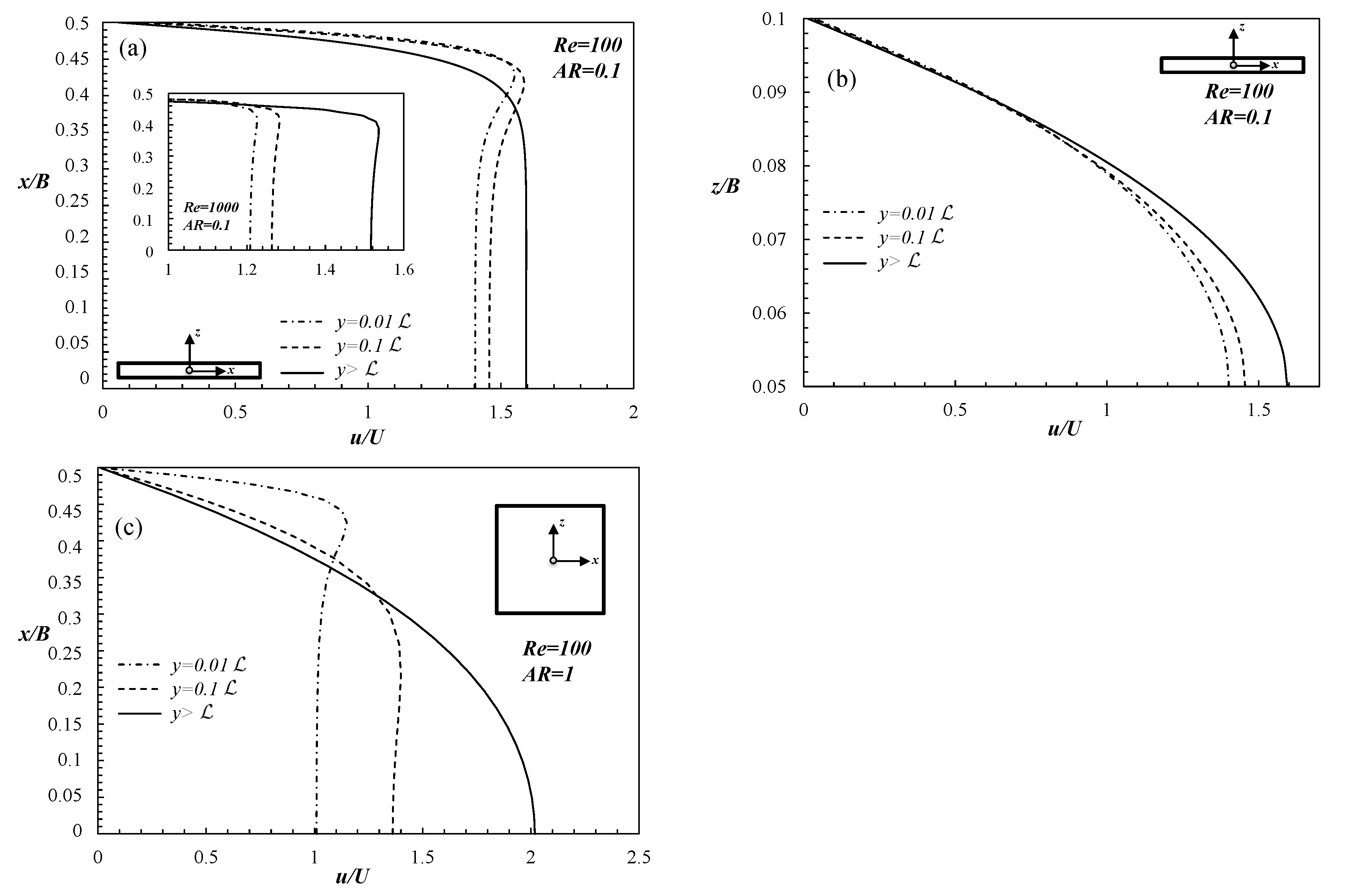
When a fluid enters a rectangular channel, the initial uniform velocity profile is gradually redistributed, accelerating around the centerplane(s) and de-accelerating near the walls. The fluid will reach a location after which the velocity profile no longer changes in all directions, and under such conditions the flow is considered to be fully developed.

Estimating this entrance length, also called development length, is one of the classical problems in fluid mechanics with practical use in microsystems design and studies of transition to turbulence [10]. Here, following the criteria proposed by Shah and London [11], the normalized development length, $\mathcal{L}=L/B$, is defined as the non-dimensional distance measured from the entrance of the microchannel, where the velocity profile is uniform, up to the axial location where the flow reaches 99% of the corresponding fully developed velocity profile. Many analytical, experimental and numerical works on the development length problem have been published over the years [11,12,13,14].

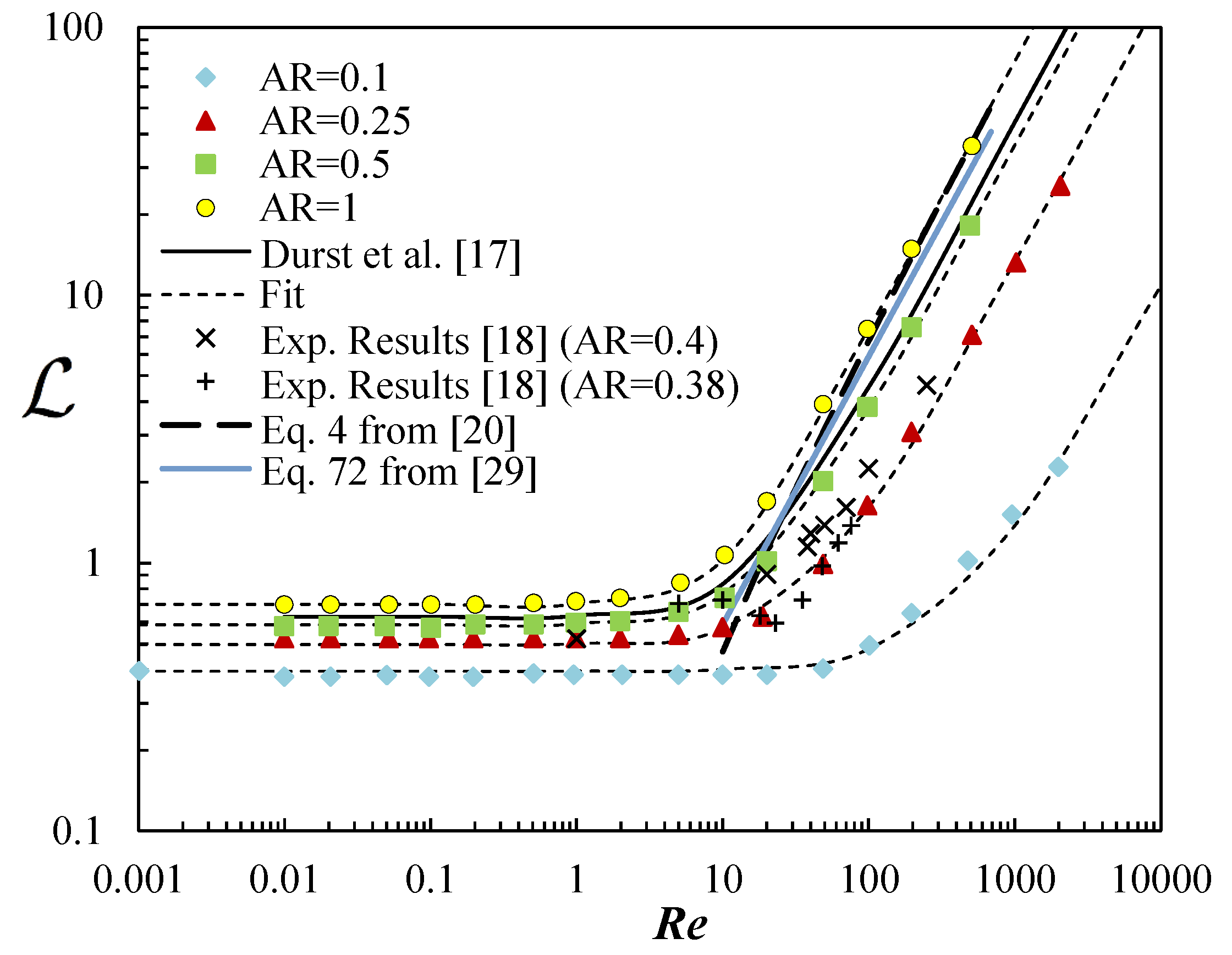
Most of the previous works proposed a linear functional relation between the development length and Reynolds number, $\mathcal{L}=C_1+C_{2}Re$, in which $C_1$ represents the asymptotic limit in the creeping flow regime, $Re\to 0$. The proposed values for $C_1$ in the literature are scattered, with the linear correlation hardly predicting the development length accurately for low Reynolds number flows (see Table 1).

Table 1. Existing correlations to estimate $\mathcal{L}=f\left(Re\right)$ for low $Re$ channel flows between parallel plates ($Re=\rho U{L}^{*}/\eta$, with $L^{*}$ representing the channel width). num. and exp. stand for numerical and experimental work, respectively.

Reference	Type	Geometry	$\mathcal{L}=\mathit{f}\left(\mathbf{Re}\right)$	${\mathit{C}}_1$	${\mathit{C}}_2$	${\mathit{C}}_3$	$\mathit{R}\mathit{e}$ Range
Atkinson et al. [15]	num.	planar channel	$\mathcal{L}=C_1+C_{2}Re$	0.625	0.044	-	$(0,1000]$
Chen [16]	num.	planar channel	$\mathcal{L}=\frac{C_1}{1+C_{2}Re}+C_{3}Re$	0.63	0.035	0.044	$(0,\mathrm{10,000}]$
Durst et al. [17]	num.	planar channel	$\mathcal{L}={\left(C_1^{C_3}+{\left(C_{2}Re\right)}^{C_3}\right)}^{\frac{1}{C_3}}$	0.631	0.0442	1.6	$(0,1000]$
Lee et al. [18]	exp.	rectangular channel	$\mathcal{L}=\frac{C_1}{1+C_{2}Re}+C_{3}Re$	0.46	0.011	0.013	$(0,100]$
Ahmad and Hassan [19]	exp.	rectangular channel	$\mathcal{L}=\frac{C_1}{1+C_{2}Re}+C_{3}Re$	0.55	0.13	0.065	$(0,1000]$
Lobo and Chatterjee [20]	num.	square channel	$\mathcal{L}=C_{1}Re-C_{2}R{e}^{C_3}$	0.077	0.096	0.5	$(20,500]$

The Reynolds number is defined in this work as $Re=\rho UB/\eta$ and the aspect ratio is $AR=H/B$, where B is chosen as the larger side and H as the smaller side of the rectangular channel (see Figure 1), thus in all cases $0<AR\le 1$.

Remark 1.

It should be noted that, to present a correlation where the results for the different $AR$ can be comparable, the dimension B was used as the characteristic length scale in all dimensionless development lengths. This means that this correlation cannot be compared with the one from Durst et al. [17], for planar channels, $AR\to 0$. We define $Re=\rho UB/\eta$ and $R{e}_H=\rho UH/\eta$, thus $R{e}_H=AR\times Re$. Note also that the Reynolds based on the hydraulic diameter ($D_h$) is given by $R{e}_{D_h}=\rho U{D}_h/\eta$, with $D_h=2BH/(B+H)$. Therefore, we have $R{e}_{D_h}=Re[2H/(B+H)]$. For a square duct, $B=H$ and $R{e}_{D_h}=Re$.

The nonlinear behaviors of the entrance length with respect to the Reynolds number for pipe and parallel plate flows were first investigated by Atkinson et al. [15], using a linear combination of creeping flow with boundary-layer type solutions, and Chen [16], using the integral momentum method to derive approximate solutions for the development length. The resulting functional relations for $\mathcal{L}$ in planar channel flows are listed in Table 1, along with the appropriate fitting constants. These nonlinear correlations indicate that the development length has a rational relationship with the Reynolds number when the Reynolds number is small, with $\mathcal{L}$ approaching a constant value as $Re\to 0$.

When the Reynolds number increases, the constant and rational portions become less dominant and the entrance length variation with $Re$ becomes linear.

Sadri and Floryan [21] presented a linear correlation for the relation of $\mathcal{L}\left(Re\right)$ ranging from $Re=0.01$ to 2200. They relied on a numerical method based on the use of the stream function and vorticity in the flow governing equations, with a compact fourth-order finite-difference scheme. The values of their correlation overpredict the entry length at low $Re$ due to the omission of the upstream flow development and at high values of $Re$ due to the omission of flow separation effects (they decoupled the upstream and downstream regions of channel entry). Sadri and Floryan also compared different definitions of the entry length and studied their influence on the obtained development lengths of the flow.

More recently, Durst et al. [17] improved the linear functional prediction accuracy by superimposing diffusion and convection together in their model while suggesting a method to determine the normalized entrance length in laminar pipe and planar channel flows. It should be noted that, in the works previously cited, 3D effects were neglected.

Recent experimental fluid flow analysis, focused in microchannels with rectangular and square cross-sections [18,19], also present nonlinear correlations for $\mathcal{L}$ as a function of $Re$. Their conclusion is that the development lengths were found to be shorter than classical correlations found in [17]. The explanation for this difference is based on the effect of the aspect ratio, the different off-center velocity maxima of the inlet profiles and due to the pre-development of the axial velocity. Recently, Lobo and Chatterjee [20] presented a numerical study on the development of flow in a square mini-channel, taking into account the effect of flow oscillations. They also performed a steady-state study and proposed a correlation for the development length for a square microchannel.

In this work, we present a detailed numerical investigation on the development length ($\mathcal{L}=L/B$) in rectangular microchannels by considering the laminar regime (including the limit of creeping flow conditions) and the dependence on the aspect ratio, $AR$.

It should be remarked that, although some works dedicate particular attention to the effects of surface roughness, wettability and the presence of gaseous layers (thus multiphase flows) leading to interfacial slip typical of some specific fluids and particular conditions [22], here we assume a single phase fluid and that the quality of manufacturing is sufficiently good to ensure smooth surfaces (as in channels made of PDMS through soft lithography [23] or made from fused-silica glass [24] so that the no-slip boundary condition remains valid).

The remainder of this work is organized as follows. In the next section, we present the governing equations, the numerical method and computational meshes used in the simulations. In Section 3, we present the results and discussion. The paper ends with the main conclusions.

2. Governing Equations, Numerical Method and Computational Meshes

To predict the developing flow field within the microchannel, we assume that the flow is three-dimensional, laminar, isothermal, incompressible and steady. The governing equations for such conditions are those expressing conservation of mass,

$$\nabla ·\mathbf{u}=0,$$

(1)

and the momentum equation,

$$\rho \left(\frac{\partial \mathbf{u}}{\partial t}+\nabla ·\mathbf{u}\mathbf{u}\right)=-\nabla p+\nabla ·\mathbf{\tau }$$

(2)

where $\mathbf{u}$ is the velocity vector, p is the pressure, t is the time, $\rho$ is the fluid density and $\mathbf{\tau }$ is the Newtonian extra stress tensor, defined as:

$$\mathbf{\tau }=\eta \left(\nabla \mathbf{u}+\nabla {\mathbf{u}}^T\right)=2\eta \mathbf{D}$$

(3)

with $\mathbf{D}$ representing the symmetric rate of strain tensor and $\eta$ the dynamic viscosity. An in-house finite-volume method code (FVM) was used in this numerical study (for more details, see [25,26]). In this code, all diffusive terms are discretized using second-order central differences, and the advective term in the momentum equation is discretized with the CUBISTA high-resolution scheme [25], which is formally of third-order accuracy. The term $\nabla ·\mathbf{\tau }$ in Equation (2) is usually represented as $\eta {\nabla }^2\mathbf{u}$ in Newtonian fluid flows, but our numerical method is also applicable for more complex fluids and uses the stress tensor notation.

The channel geometry is represented in Figure 1. A uniform velocity, U, is imposed at the inlet ($y/B=0$) of the microchannel, where all other velocity components and deviatoric stresses are set to zero. Vanishing streamwise gradients are applied to all variables at the outlet plane, except for the pressure, which is linearly extrapolated to the outlet from the two nearest upstream cells. The classical no-slip condition is imposed at the channel walls.

The iterative time stepping procedure was stopped whenever the $L_2-norm$$\left(\sqrt{{\sum }_{i=1}^n{\left|x_i\right|}^2}\right)$ of the residuals vector of the system of equations was less than a tolerance of ${10}^{-8}$, which corresponds to steady-state flow. The calculations for the creeping flow limiting case, $Re\to 0$, were carried out by dropping out the convective term of the momentum equation.

In order to achieve mesh-independent results, the full physical domain depicted in Figure 1 was discretized into eight different sets of computational domains, with consecutively refined meshes. A detailed summary of those meshes is presented in Table 2. To avoid an effect of the computational domain on the calculated development length, the microchannel was made significantly longer than the value of $\mathcal{L}$, so that, at the end, the length of the microchannel domain varied between four and twenty times the calculated development length. In turn, this depended also on the Reynolds number. The number of cells ($NC$) in the axial direction increased with the length of the computational domain, and a non-uniform distribution of the cells sizes was used, with the ratio of the geometric progression of the cell spacing equal to 1.04040 for meshes M1, M2, M3, M4, M9, M10, M11 and M12 and 1.02 in meshes M5, M6, M7, M8, M13, M14, M15 and M16.

Table 2. Details of the channel meshes used in the accuracy tests.

${\mathit{L}}_{\mathit{C}}/\mathit{B}$	$\mathit{H}/\mathit{B}$	Mesh	$\mathbf{NC}(\mathit{y}\times \mathit{z}\times \mathit{x})$	$\mathit{\Delta }{\mathit{y}}_{\mathbf{min}}/\mathit{B}$	$\mathbf{\Delta }{\mathit{z}}_{\mathbf{min}}/\mathit{B}$
10	0.1	$M_1$	25 × 51 × 11	0.0660	0.0095
	0.25	$M_2$	50 × 21 × 21	0.0323	0.0119
	0.5	$M_3$	50 × 21 × 21	0.0324	0.0238
	1	$M_4$	50 × 21 × 21	0.0324	0.0476
10	0.1	$M_5$	50 × 101 × 21	0.0324	0.0048
	0.25	$M_6$	100 × 41 × 41	0.0160	0.0061
	0.5	$M_7$	100 × 41 × 41	0.0160	0.0122
	1	$M_8$	100 × 41 × 41	0.0160	0.0244
100	0.1	$M_9$	96 × 51 × 11	0.0660	0.0095
	0.25	$M_{10}$	191 × 21 × 21	0.0324	0.0119
	0.5	$M_{11}$	191 × 21 × 21	0.0324	0.0238
	1	$M_{12}$	191 × 21 × 21	0.0324	0.0476
100	0.1	$M_{13}$	191 × 101 × 21	0.0323	0.0048
	0.25	$M_{14}$	381 × 41 × 41	0.0160	0.0061
	0.5	$M_{15}$	381 × 41 × 41	0.0160	0.0122
	1	$M_{16}$	381 × 41 × 41	0.0160	0.0244

For the x direction, the cells were uniformly distributed with the total number of cells, NC, shown in Table 2. The present mesh refinement strategy was designed in order to provide a consistent estimate of uncertainty of our simulations using Richardson’s extrapolation technique [27]. This method allows us to estimate the mesh independent extrapolated development length (${\mathcal{L}}_{ext}$) as ${\mathcal{L}}_{ext}={\mathcal{L}}_{M4}+({\mathcal{L}}_{M4}-{\mathcal{L}}_{M3})/(2^p-1)$ based on our numerical simulations in meshes M3 and M4, for the sake of example, where p is the order of accuracy of the computations. Assuming a second-order accuracy, $p=2$, ${\mathcal{L}}_{ext}$ can be estimated as ${\mathcal{L}}_{ext}={\mathcal{L}}_{M4}+({\mathcal{L}}_{M4}-{\mathcal{L}}_{M3})/3$.

This technique also allows us to estimate the accuracy of a specific calculation, defined as

$$e_{R,M_i}=\frac{|{\mathcal{L}}_{ext}-{\mathcal{L}}_i|}{{\mathcal{L}}_{ext}}.$$

(4)

where ${\mathcal{L}}_i$ is the length computed numerically in mesh $M_i$. In addition to the mesh-dependency study, another parameter used for estimating the accuracy in this work is the velocity relative error ($e_{u,M_i}$) for mesh $M_i$, defined as,

$$e_{u,M_i}=\frac{u_{max,num}-u_{max,theo}}{u_{max,theo}},$$

(5)

where $u_{max,num}$ is the predicted maximum velocity at the outlet plane and $u_{max,theo}$ is the corresponding fully developed theoretical maximum velocity value computed using the analytical solution [28].

It should be remarked that preliminary tests with different meshes where conducted initially, in order to select the most appropriate meshes, without compromising the convergence accuracy and the computational time needed to perform the simulations.

3. Results and Discussion

3.1. The Development Length

In order to estimate $\mathcal{L}$, simulations were conducted from small $Re$ (creeping flow conditions) up to $Re=2000$, covering the laminar regime. Note that for high AR the simulations were performed for lower values of $Re$, so that the flow stays laminar (see, e.g., [18]).

The computational domain size of the microchannel for the 3D flow field is shown in Table 2. A square section ($AR$ = 1) and three additional rectangular sections with $AR=0.5$, $AR=0.25$ and $AR=0.1$ were investigated.

The results obtained for ${\mathcal{L}}_{ext}$ considering different $AR$ are presented in Table 3, for a number of representative $Re$ values. It should be remarked that the errors are below 3.5%, within the asymptotic range of convergence (see Appendix A, Table A1, Table A2, Table A3 and Table A4 for a detailed study on the error for the different meshes and $AR$).

Table 3. Values of ${\mathcal{L}}_{ext}$ for different $Re$ and $AR$.

$\mathbf{Re}$	${\mathcal{L}}_{\mathbf{ext}}$
	$\mathbf{AR}=\mathbf{0}.\mathbf{1}$	$\mathbf{AR}=\mathbf{0}.\mathbf{25}$	$\mathbf{AR}=\mathbf{0}.\mathbf{5}$	$\mathbf{AR}=\mathbf{1}$
0.001	0.3945	0.5184	0.5820	0.6907
0.01	0.3945	0.5185	0.5823	0.6908
0.02	0.3945	0.5185	0.5823	0.6902
0.05	0.3945	0.5186	0.5825	0.6915
0.1	0.3946	0.5187	0.5830	0.6924
0.2	0.3947	0.5190	0.5840	0.6942
0.5	0.3950	0.5197	0.5870	0.6997
1	0.3955	0.5212	0.5922	0.7110
2	0.3965	0.5240	0.6029	0.7363
5	0.3994	0.5347	0.6449	0.8314
10	0.4044	0.5627	0.7372	1.0636
20	0.4143	0.6385	0.9950	1.7051
50	0.4439	0.9714	2.0416	3.8671
100	0.4933	1.6614	3.8916	7.5320
200	0.5922	3.0721	7.5692	14.8345
500	0.8887	7.0889	18.4299	36.4319
1000	1.3829	13.4546	-	-
2000	2.3713	25.7523	-	-

The values of ${\mathcal{L}}_{ext}$ in simulations up to $Re$ = 20, 100, 500 and 2000 performed in meshes M1–M4, M5–M8, M9–M12 and M13–M16, respectively, are shown to be independent of the length of the computational domain, as observed in the values of ${\mathcal{L}}_{ext}$ presented in Table A1, Table A2, Table A3 and Table A4.

The data shown in Table 3 can be better understood by looking at Figure 2. A decrease of the development length with the decrease of $AR$ is observed for the whole range of $Re$ considered. For creeping flow, we note a more pronounced decrease of $\mathcal{L}$ as $AR$ deviates from $AR=1$. For low $Re$, the difference in the development length for the different $AR$ is less significant when compared with the results obtained for high $Re$. For high $Re$, convection starts to play an important role, and, to understand this flow behavior, the local velocity profiles must be analyzed.

Figure 2. Development length $\mathcal{L}$ for different $AR$, compared against the experimental results given in [18]. The dashed lines show the fit obtained with the correlation given in Equation (6). We also show a comparison with the correlation proposed in [20], and a good agreement is observed (except for low $Re$ where the correlation proposed by [20] fails). The correlation proposed in [29] also shows good agreement with the correlation proposed in [20] (in [20], several correlations are developed to account for different duct shapes).

Note that we also compare our results with the experimental data of Lee et al. [18] for $AR=0.4$ and $0.38$. The experimental results are qualitatively in agreement with our numerical predictions.

3.2. Flow Dynamics

Figure 3a,c shows non-dimensional transverse profiles of streamwise velocity at various streamwise locations y for $Re=0.001$ (creeping flow) and two different aspect ratios $AR=0.1$ and $AR=1$. Figure 4a,c shows the corresponding profiles but considering inertial effects at $Re=100$. The profiles are presented only for half of the channel due to the flow symmetry.

Figure 3. Velocity profiles obtained for $AR=0.1$ (a) and $AR=1$ (c) in the $x-$plane, for $Re=0.001$ at different y positions along the microchannel ($z=0$). (b) Velocity profiles obtained for $AR=0.1$ and $Re=0.001$ in the $z-$plane, for different y positions along the microchannel ($x=0$).

Figure 4. Velocity profiles obtained for $AR=0.1$ (a) and $AR=1$ (c) in the $x-$plane, for $Re=100$ and different y positions along the microchannel ($z=0$). The inset in (a) shows the velocity profiles obtained for the case $Re=1000$. (b) Velocity profiles obtained for $AR=0.1$ and $Re=100$ in the $z-$plane, for different y positions along the microchannel ($x=0$).

Comparing Figure 3a,c, we observe that for the lower aspect ratio the overshoot is more pronounced, possibly due to the restrictive no slip boundary condition of the top and bottom walls that are much closer to the center than the side walls. Figure 3b shows the evolution of the non-dimensional axial velocity component at several axial positions along the $z-$direction for the case of $AR=0.1$ and $Re=0.001$ (the results are qualitatively similar for other $AR$). In this case, the left and right walls are far from the development region, and we have an almost 2D case, where a more parabolic profile is obtained.

The overshoots are generated as a result of the abrupt local fluid deceleration near the channel wall at the inlet section due to the no-slip boundary condition. Since the fluid near the symmetry axis is not accelerated immediately, whereas the fluid near the wall is stationary as soon as it enters the inlet region, to satisfy the continuity equation, velocity overshoots are formed near the wall, close to the inlet section. This behavior was also reported by Durst et al. [17] for Newtonian fluids in 2D channels.

We can also observe that there is a dependence on the development of the axial velocity with $Re$, with the increase of inertia leading to longer axial development lengths to achieve fully developed flow (see also Figure 2). The non-dimensional axial velocity component presents a local maximum that becomes more pronounced and closer to the channel walls as the Reynolds number increases.

By comparing the evolution of the non-dimensional axial velocity component at several axial positions along the $z-$direction for the case of $AR=0.1$ and $Re=\{0.001,100\}$, we observe that near the entrance the case of $Re=0.001$ shows a more pronounced development, while the combination of inertia/diffusion effects requires higher $\mathcal{L}$ to stabilize the flow field in the case of $Re=100$ (see Figure 3b and Figure 4c).

The evolution of the non-dimensional streamwise velocity along the center of the duct is shown in Figure 5 for creeping flow conditions and $Re=100$ for $AR=1$. The development of the axial velocity profiles is not linear, following a logistic-type function behavior. Initially, the fluid evolves slowly as a plug (before the the momentum diffusion from the wall reaches the center) and then quickly evolves to its fully developed value. This occurs for both values of $Re$ considered, but, as expected, achieving the fully developed regime takes higher $\mathcal{L}$ when convection plays an important role.

Figure 5. Axial velocity development along the $y-$axis in the centerline $(x=0,z=0)$ for $AR=1$ and $Re=\{0.001,100\}$.

3.3. Entrance Length Correlation

In order to obtain a nonlinear correlation between $\mathcal{L}$ and $Re$, we performed a fit to the numerical results shown in Table 3. The following correlation, valid in the ranges $0\le Re\le 2000$ and $0.1\le AR\le 1$, was obtained:

$$\mathcal{L}={\left(C_1^{C_3}+{\left(C_{2}Re\right)}^{C_3}\right)}^{\frac{1}{C_3}}$$

(6)

The correlation follows the same structure of the one proposed by Durst et al. [17], but now $C_1$, $C_2$ and $C_3$ are functions of $AR$. For the range of $AR$ studied in this work, we obtained the following functions:

$$\left\{\begin{array}{c}{C}_1=0.7A{R}^{0.25}\\ \\ C_2={\displaystyle \frac{6.8A{R}^{3.75}}{1+90A{R}^{2.8}}}\\ \\ C_3=1+AR\end{array}\right.$$

(7)

An overall average relative error of $2.2\%$ and a maximum relative error of $6.0\%$ were obtained, and the good quality of fit is shown in Figure 2 (dashed lines).

4. Conclusions

An extensive and systematic numerical study was carried out regarding the entrance length, $\mathcal{L}$, for Newtonian fluids in 3D microchannels with rectangular cross section. An adequate choice of meshes, with consistent mesh refinement, and accurate numerical methods allowed the prediction of accurate values of $\mathcal{L}$, and a unified nonlinear correlation was proposed for estimating $\mathcal{L}$, valid in laminar regime for $0\le Re\le 2000$ and $0.1\le AR\le 1$. This correlation allows an accurate prediction of entrance length and represents a novel tool for the design and fabrication of efficient microfluidic devices.

References

- Bayraktar, T.; Pidugu, S.B. Characterization of liquid flows in microfluidic systems. Int. J. Heat Mass Transf. 2006, 49, 815–824. [Google Scholar] [CrossRef]
- Talimi, V.; Muzychka, Y.S.; Kocabiyik, S. A review on numerical studies of slug flow hydrodynamics and heat transfer in microtubes and microchannels. Int. J. Multiphase Flow 2012, 39, 88–104. [Google Scholar] [CrossRef]
- Morini, G.L.; Yang, Y.; Chalabi, H.; Lorenzini, M. A critical review of the measurement techniques for the analysis of gas microflows through microchannels. Exp. Therm. Fluid Sci. 2011, 35, 849–865. [Google Scholar] [CrossRef]
- Saisorn, S.; Wongwises, S. A review of two-phase gas-liquid adiabatic flow characteristics in micro-channels. Renew. Sustain. Energy Rev. 2008, 12, 824–838. [Google Scholar] [CrossRef]
- Hetsroni, G.; Mosyak, A.; Pogrebnyak, E.; Yarin, L.P. Heat transfer in micro-channels: Comparison of experiments with theory and numerical results. Int. J. Heat Mass Transf. 2005, 48, 5580–5601. [Google Scholar] [CrossRef]
- Duan, Z.; Muzychka, Y.S. Slip flow in elliptic microchannels. Int. J. Therm. Sci. 2007, 46, 1104–1111. [Google Scholar] [CrossRef]
- Kuddusi, L.; Çetegen, E. Thermal and hydrodynamic analysis of gaseous flow in trapezoidal silicon microchannels. Int. Therm. Sci. 2009, 48, 353–362. [Google Scholar] [CrossRef]
- Eskin, D.; Mostowfi, F. A model of a bubble train flow accompanied with mass transfer through a long microchannel. Int. Heat Fluid Flow 2012, 33, 147–155. [Google Scholar] [CrossRef]
- Quan, X.; Dong, L.; Cheng, P. Determination of annular condensation heat transfer coefficient of steam in microchannels with trapezoidal cross sections. Int. J. Heat Mass Transf. 2010, 53, 3670–3676. [Google Scholar] [CrossRef]
- Poole, R.J.; Chhabra, R.P. Development Length Requirements for Fully Developed Laminar Pipe Flow of Yield Stress Fluids. J. Fluids Eng. 2010, 132, 034501. [Google Scholar] [CrossRef]
- Shah, R.K.; London, A.L. Laminar Flow Forced Convection in Ducts: A Source Book for Compact Heat Exchanger Analytical Data; Academic Press: New York, NY, USA, 1978. [Google Scholar]
- Schiller, L. Die Entwicklung der laminaren Geschwindigkeitsverteilung und ihre Bedeutung für Zähigkeitsmessungen. (Mit einem Anhang über den Druckverlust turbulenter Strömung beim Eintritt in ein Rohr). J. Appl. Math. Mech. 1922, 2, 96–106. [Google Scholar] [CrossRef] [Green Version]
- Schlichting, H.; Kestin, J. Boundary Layer Theory; McGraw-Hill: New York, NY, USA, 1979. [Google Scholar]
- Collins, M.; Schowalter, W.R. Behavior of non-Newtonian fluids in the inlet region of a channel. AIChE J. 1963, 9, 98–102. [Google Scholar] [CrossRef]
- Atkinson, B.; Brocklebank, M.P.; Card, C.C.; Smith, J.M. Low Reynolds number developing flows. AIChE J. 1969, 15, 548–553. [Google Scholar] [CrossRef]
- Chen, R.-Y. Flow in the Entrance Region at Low Reynolds Numbers. J. Fluids Eng. 1973, 95, 153–158. [Google Scholar] [CrossRef]
- Durst, F.; Ray, S.; Ünsal, B.; Bayoumi, O.A. The Development Lengths of Laminar Pipe and Channel Flows. J. Fluids Eng. 2005, 127, 1154–1160. [Google Scholar] [CrossRef]
- Lee, S.-Y.; Jang, J.; Wereley, S. Effects of planar inlet plenums on the hydrodynamically developing flows in rectangular microchannels of complementary aspect ratios. Microfluid. Nanofluidics 2008, 5, 1–12. [Google Scholar] [CrossRef]
- Ahmad, T.; Hassan, I. Experimental Analysis of Microchannel Entrance Length Characteristics Using Microparticle Image Velocimetry. J. Fluids Eng. 2010, 132, 041102. [Google Scholar] [CrossRef]
- Lobo, O.J.; Chatterjee, D. Development of flow in a square mini-channel: Effect of flow oscillation. Phys. Fluids 2018, 30, 042003. [Google Scholar] [CrossRef]
- Sadri, R.M.; Floryan, J.M. Entry flow in a channel. Comput. Fluids 2002, 31, 133–157. [Google Scholar] [CrossRef]
- Chiara, N.; Evans, D.R.; Bonaccurso, E.; Butt, H.-J.; Craig, V.S.J. Boundary slip in Newtonian liquids: A review of experimental studies. Rep. Prog. Phys. 2005, 68, 2859. [Google Scholar]
- Campo-Deaño, L.; Dullens, R.P.A.; Aarts, D.G.A.L.; Pinho, F.T.; Oliveira, M.S.N. Viscoelasticity of blood and viscoelastic blood analogues for use in PDMS (polydymethylsiloxane) in vitro models of the circulatory system. Biomicrofluidics 2013, 7, 34102. [Google Scholar] [CrossRef] [PubMed] [Green Version]
- Pimenta, F.; Toda-Peters, K.; Shen, A.Q.; Alves, M.A.; Haward, S.J. Viscous flow through microfabricated axisymmetric contraction/expansion geometries. Exp. Fluids 2020, 61, 1–16. [Google Scholar] [CrossRef]
- Alves, M.A.; Oliveira, P.J.; Pinho, F.T. A convergent and universally bounded interpolation scheme for the treatment of advection. Int. J. Numer. Methods Fluids 2003, 41, 47–75. [Google Scholar] [CrossRef]
- Oliveira, P.J.; Pinho, F.T.; Pinto, G.A. Numerical simulation of non-linear elastic flows with a general collocated finite-volume method. J. Non-Newton. Fluid Mech. 1998, 79, 1–43. [Google Scholar] [CrossRef] [Green Version]
- Richardson, L.F. The Approximate Arithmetical Solution by Finite Differences of Physical Problems Involving Differential Equations, with an Application to the Stresses in a Masonry Dam. R. Lond. Philos. Trans. Ser. A 1911, 210, 307–357. [Google Scholar]
- White, F.M. Viscous Fluid Flow; McGraw-Hill: New York, NY, USA, 2006; Volume 3. [Google Scholar]
- Muzychka, Y.S.; Yovanovich, M.M. Pressure Drop in Laminar Developing Flow in Noncircular Ducts: A Scaling and Modeling Approach. J. Fluid. Eng. 2009, 131, 11105. [Google Scholar] [CrossRef]
Publisher’s Note: MDPI stays neutral with regard to jurisdictional claims in published maps and institutional affiliations. |
© 2021 by the authors. Licensee MDPI, Basel, Switzerland. This article is an open access article distributed under the terms and conditions of the Creative Commons Attribution (CC BY) license (https://creativecommons.org/licenses/by/4.0/).