Abstract
This work aims at investigating numerically the effects of channel corrugation in two-phase flows with single and multiples drops subject to buoyancy-driven motion. A state-of-the-art model is employed to accurately compute the dynamics of the drop’s interface deformation using a modern moving frame/moving mesh technique within the arbitrary Lagrangian–Eulerian framework, which allows one to simulate very large domains. The results reveal a complex and interesting dynamics when more than one drop is present in the system, leading eventually in coalescence due to the amplitude of the corrugated sinusoidal channel and distance between drops.
1. Introduction
Two-phase flows with variable cross section still remain a challenging subject with great interest from the scientific community and industry related to the efficient cooling of computer parts and biomedical devices. Moreover, channels with different corrugation patterns seem to considerably improve the effect of heat dissipation by modifying the drop’s dynamics and thus the liquid film thickness of the two-phase system. Corrugated channel is a class of variable cross section channels that present a periodic pattern along its length and has strong impact in the fluid flow, changing its behavior by increasing recirculation zones and eventually leading to onset of boundary layer detachment. Note that the presence of a deformable interface due to the presence of more fluid phases brings an extra degree of complexity in the fluid flow system. Additionally, the periodic pattern of the corrugated channels requires very large domains to be analyzed, thus dramatically increasing the costs associated to the experiment assembling or the numerical simulations.
Single-phase flows with heat transfer were experimentally analyzed in [1,2], where the effects of several key parameters were studied such as channel wavy amplitude and flow velocity in periodic wavy passages. Numerically, several authors have investigated single-phase flows in corrugated channels. For instance, in [3] a numerical study was done for transition regimes from laminar to turbulent when convective heat transfer plays an important role in those flows. They concluded that the Nusselt number for the wavy wall channel was directly affected when compared to those for a straight channels, while in [4], a 2-dimensional laminar steady and time-dependent fluid flow solver was developed for heat transfer in periodic wavy channels with sinusoidal and arc shapes. It was concluded that the arc-shaped periodic channel enhances heat transfer due to a higher friction factor when compared to the sinusoidal channel, specially beyond the critical value of the Reynolds number for the unsteady regime. Another interesting numerical approach was suggested by the authors of [5], where the coordinate transformation method and the spline alternating-direction implicit method was used to study the rates of heat transfer for flow through a sinusoidally curved converging–diverging channel. The steady streamfunction vorticity formulation was used to model the fluid flow with the energy equation using the finite difference method. Several channel amplitude wavelengths were tested at different Reynolds number, and it was found that at a sufficiently larger value of amplitude wavelength ratio the corrugated channel increases heat transfer for large Reynolds numbers. Turbulent forced convection in a wavy channel using a two-phase model was studied in [6] for water-AlO nanofluids using a 2-dimensional numerical solver. It has been seen that if the channel amplitude increases, as well as the Reynolds number and volume fraction of nanoparticles, the Nusselt number is directly affected, leading to a higher value. Additionally, it was observed that the more nanoparticles added to the solution, the higher pressure drop in corrugated channels is seen.
It is already known that two-phase flows bring another level of challenges numerically and experimentally due to the presence of an interface between fluids and different phases in the system. In [7], a comparative analysis of two-phase flow in sinusoidally corrugated channels was carried out with application to polymer electrolyte membrane fuel cells. Different patterns of corrugated channels were used to numerically analyze single and multiples bubbles dynamics in air–water systems through a 3-dimensional simulation using the Volume-of-Fluid (VOF) method. The authors concluded that the two-phase flow performance in the sinusoidal channels can be substantially improved, decreasing the radius of curvature at the bends and making the confining walls extremely hydrophobic. On the other hand, in [8], experimental and numerical approaches have been used to tackle CO bubble behavior flowing in a methanol solution in sinusoidally corrugated channels for fuel cell purposes. A detailed investigation of key two-phase flow parameters was undertaken, and a thermal analysis was made regarding when a single bubble travels along sinusoidal channels under pressure differences between the inlet and outlet regions of the channel. Additionally, a comparison of the same flow condition was carried out for a straight channel. The results reveals that the effect of flow disturbance structure is negligible with small values of channel amplitude and angular frequency of corrugation for the studied two-phase system. Sinusoidal channels with one and more wavy patterns were numerically simulated using the front-tracking and the finite volume methods in [9]. Two-phase 2-dimensional flow simulations were carried out to investigate single buoyant drops in channel constrictions and expansions and the interaction between two small drops in different simulation conditions with the newly implemented numerical code. Results have been successfully reported for various constricted channels.
The current study is based upon the experiments in [10], where the authors have studied experimentally the effects of buoyancy-driven motion of drops in a periodically constricted capillary. Several two-phase systems were used in the experiment such as glycerol–water, diethylene glycol, and diethylene glycol–glycerol as suspending fluid, and silicon oil, Dow Corning fluids, and UCON fluid emollient as drop fluids, and an extensive study has been reported for sinusoidal shape channels with fixed dimensionless amplitude and wavelength for single drops. However, no further investigation has been conducted for different channel amplitude and its effect on interface break-up for single and multiple drops. Additionally, it is clear from the literature review presented above that much is still required for the complete understanding of two-phase flows in short and large periodic arrays with different corrugation levels. It is indeed of great significance that single and multiple buoyant drops in sinusoidal channels deliver another level of flow complexity due to the possible significant channel amplitude perturbation in the two-phase system, leading eventually to drop coalescence and/or interface breakup. The aim of this work is to investigate numerically two-phase flow key parameters such as the drop’s rising velocity, film thickness, and interface perimeter change for one and three drops in buoyancy-driven motion for a diethylene glycol/UCON-1145 (DEG3) two-phase system in sinusoidal channels with dimensionless wavelength and wave amplitude . Additionally, a parametric study is also carried out to investigate the influence of channel wavelength and drop volume in coalescence during slug flows. A state-of-the-art model is employed to accurately compute the dynamics of the drop’s interface motion using a modern moving frame/moving mesh technique within the arbitrary Lagrangian–Eulerian framework. The presented results show the drop’s dynamics in large periodic channels and coalescence even for large liquid slug distances.
This article is organized with a literature review of single- and two-phase corrugated channels, followed by the mathematical description of the modeling equations in axisymmetric formulation based on the Finite Element Method (FEM). The next section provides details concerning the numerical modeling used to discretize the mathematical equations, followed by the result section where several important test cases are presented to assess and analyze the dynamics of two-phase flow in corrugated channels with single and multiples bubbles. Finally, this text ends with remarks in the conclusion section.
2. Mathematical Description
2.1. Two-Phase Flow Equations in the ALE Context
Momentum and continuity equations are used as the model for incompressible motion of two-phase flows in the context of a “one-fluid” description where one set of equations is used domain-wise and a jump in fluid properties is assumed at the interface. The dimensionless form of the momentum and continuity equations respectively is shown in cylindrical coordinates for axisymmetric flows with gravity and surface tension force accounted in as
where is the position vector with radial r and axial x coordinates. is the velocity vector with components and , is the mesh velocity vector with components and . The velocity difference is due to the arbitrary Lagrangian–Eulerian framework; otherwise, only is found when a fixed frame (Eulerian) is established. is the fluid density, is the fluid dynamic viscosity spatially distributed with a jump condition at the interface , is the surface tension with radial and axial components, respectively, p is pressure and t is time. Note here that the fluid properties and are dimensionless and they appear in the two-phase flow equation since both are usually different among phases; however in single-phase flows both are constant and equal to the unity, thus vanishing from the momentum equation. As flow is buoyancy-drive driven, the dimensionless groups Archimedes () and Eötvös () appear in the momentum equation according to the standard dimensional analysis and are both defined as follows,
where the subscript stands for the reference values of dynamic viscosity , surface tension , gravity , and channel diameter D. is defined as the difference of densities among phases.
2.2. Axisymmetric Differential Operators
The dimensionless axisymmetric strain tensor in the momentum equation does not account for the mesh motion itself; however, in two-phase flows, both the velocity gradient () and the gradient transpose () shall be considered due to fluid properties transition at interface, resulting in nonuniform spatially variation in density and . Therefore, it is written according to the following expression,
The divergent () and transpose gradient () defined as follows,
3. Numerical Simulation
3.1. General Description of Two-Phase Flow Solver
The current numerical methodology is based on the works in [11,12,13], and a short description is given for the sake of completeness, with detailed explanation of the triangle finite element used in this work, as well as the geometrical parameters used to assemble the numerical test sections and the finite element mesh treatment. The current numerical code has been implemented in C/C++ language using object-oriented programming with aid of PETSc framework ([14]) for the linear system solvers and preconditioners, the finite element mesh generator GMsh [15] for initial interface and boundary mesh setup, and the triangle mesh generator package Triangle [16] for adaptive remeshing support.
The classical Galerkin method has been used as approximating method to the variational formulation of the governing equations resulting in the discretization of all terms except the nonlinear advection term . Such a term is known to be the source of undesired spurious modes that may cause numerical instabilities if the Galerkin method is used. Thus, to overcome such an undesired issue, the semi-Lagrangian method [17,18] has been successfully employed in this work. The idea of representing the acceleration field by a Lagrangian framework instead of the commonly found Eulerian framework. Note that such a method is applied to the ALE convective velocity difference within the ALE framework. For each time step the nodes move towards the flow characteristics and a re-initialization of the system coordinates is performed, thus recovering the initial mesh. The substantial derivative with the ALE velocity difference is evaluated in the strong form along the characteristic trajectory, by estimating the position of a point and solving the vectorial equation backwards in time with the initial condition , where is the mesh node coordinate, than an integration method is used to evaluate the previous node position in the triangle unstructured mesh. A first order discretization scheme is adopted assuming the trajectory is linear.
The numerical domain is discretized using an unstructured triangle mesh with a LLB-stable mini-element with details given in the next section. Once the discretization of the domain is accomplished, the system matrices are assembled and the solution of the time dependent 2-dimensional axisymmetric equations is then found by successively solving the linear system using PETSc framework in each time step for pressure and velocity. However, due to the strong coupling between pressure and velocity, the numerical procedure implemented to solve the mentioned linear system uses the Projection method based on the LU decomposition, which was first introduced by [19]. The aim of this method is to uncouple pressure and velocity and solve each quantity separately, thus reducing the large linear system size into smaller ones. The solution of the linear system for pressure is given by a direct solver based on LU decomposition, and the velocity is solved by the conjugated gradient method using the incomplete Cholesky factorization as preconditioner as the associated linear system is positive symmetric definite.
3.2. Choice of the Finite Element
The linear element with cubic bubble function uses three shape functions that are interpolated at the vertex of the element supplemented by a cubic bubble function, which is interpolated at the element centroid. As only four degrees of freedom are used for a cubic polynomial, the shape functions of this element are incomplete. This element is also know as mini element. Such a scheme gives an LBB stable element without having to introduce too many degrees of freedom. The shape functions, in terms of barycentric coordinates, are
where are the shape functions of the corner nodes of the mini-triangle element Figure 1b, and is the shape functions of the triangle centroid node. The associated boundary element is a linear line element and its shape functions are simply the functions of the barycentric coordinates and . As can be seen in Figure 1, the combination of both triangles generates the well-known mini-element, which is LBB stable and does not require any additional term in the fluid motion equations. The linear element was used to evaluate pressure at the corner nodes and mesh update procedure, while the mini and linear boundary elements were used to evaluate velocity at all element nodes.
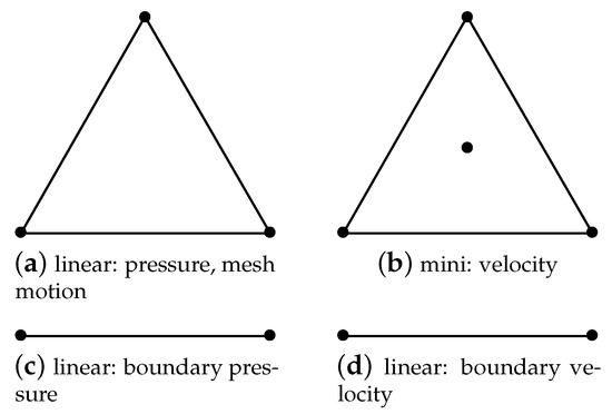
Figure 1.
Interpolation nodes for the triangle finite elements and boundary finite elements used in the current work. The linear element was used to evaluate pressure at the corner nodes and mesh update, while the mini and linear boundary element were used to evaluate velocity at all element nodes. The combination of these two triangle elements generates the finite element.
3.3. Test Sections
Two numerical test sections were used in the present work, namely, straight and sinusoidal channels. Each test section was tested with single-drop flow and consecutive three-drop flow with different liquid slug thickness s, as can be seen in Figure 2; thus, resulting in a simplified slug flow pattern where the center drop’s flow is directly affected by the front and rear drop’s motion. If the amplitude of the sinusoidal channel is set to , one achieves the straight channel, and the same numerical method and mesh can be used; therefore, allowing the investigation of the influence of channel wall into the drop’s dynamics. The sinusoidal wall profile is set through the harmonic wave equation:
where is the channel’s diameter and is its radius; is the wave amplitude that was set to for the straight and sinusoidal channels, respectively; is the wavelength; and is its phase. The axial coordinate is x, while refers to the drop’s referential point. The moving boundary approach has been discussed in details in [12], where the drop or drops center of mass remain fixed in space while the boundary moves according to its position increment with time. Such a procedure has been successfully proven to be efficient and allowing large periodic domain to be simulate with low computational costs. Additionally, four dimensionless liquid slug lengths, s, have been used: , thus varying significantly the axial distance between drops. The drop’s size factor relative to the channel’s radius () was used to set the drop’s dimension for all simulations presented in this work. The chosen drop’s size factor implies a drop with a radius of times the channel’s radius by considering the equivalent radius of a spherical drop with same volume. It is important to note that the initial drop’s shape presents a approximated drop’s shape found in two-phase flows in channels (see, e.g., in [20,21,22]).
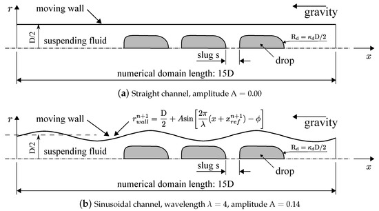
Figure 2.
Geometries of the straight and sinusoidal channels used in this work. Note that the straight channel is obtained by setting the amplitude of the sinusoidal channel to . One and three drops were used in this work, with liquid slug s of where is the drop’s diameter. is the drop’s size factor relative to the channel’s radius () where the following relation remains , with as the drop’s radius. All parameters are dimensionless.
3.4. Mesh Treatment
The numerical code solves the fluid motion equations using a moving mesh technique within the ALE framework, which requires an efficient adaptive mesh refinement when large mesh deformation occurs. It is important to note that the current code implementation moves the mesh nodes and decides whether deletion or insertion of nodes and elements is required; however, the connective matrix needed by the FEM solver is generated using the package Triangle. The spatial mesh node distribution is given through the solution of the generalized Helmholtz equation for the whole domain, and the decision whether to insert or delete nodes is performed based upon a given predefined tolerance. The solution is numerically obtained using the FE method using the classical discrete operators with the triangle linear element.
Figure 3 presents a detailed view of the unstructured triangle finite element mesh using during the simulation of three drops flow in axisymmetric sinusoidal channel, where the bottom boundary stands for the axis of symmetry. It illustrates in details the resulting mesh during the corrugated channel passage of two sequential drops with large interface deformation. Furthermore, recall that an extra centroid node is used in the calculation of the velocity field that is not appearing in the current figure. As can be seen, the minimum liquid film thickness in the front drop is covered by a minimum of 5 triangle elements and 9 nodes; thus, capturing accurately the dynamics within such an important region in two-phase flows. Not less important, the unstructured triangle mesh is updated every time step due to the Lagrangian motion of the interface nodes as well as the phase nodes, both using the mesh velocity . It is indeed noticeable that insertion and deletion of nodes as well as flipping of triangle edges are required to complete the mesh treatment and maintain consistence of the numerical algorithm thus resulting in an accurate method to track interface motion under high deformation.
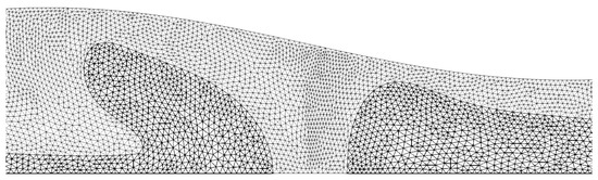
Figure 3.
Unstructured triangle finite element mesh detailed of slug flow in sinusoidal channel. This figure illustrates, in detail, the resulting mesh during the corrugated channel passage of two sequential drops. The left hand side drop is deformed during the convergent section, while the right hand side is stretched out when passing by the convergent section. Black lines of triangles represent the inner region (drops) and the others stand for the outer region (suspending fluid).
4. Results
We present the results of single and multiples drops rising in channels with two levels of corrugation amplitude () obtained with the ALE-FE Two-Phase flow solver for axisymmetric coordinate system. Note that such a code has been extensively validated against several single and two-phase flows problems and have been reported in different well-recognized international journals. All numerical results presented here refers to fluid the two-phase system diethylene glycol/UCON-1145 from [10] also known as DEG3 system. According to the experiments, the drop fluid (UCON-1145) presented the dynamic viscosity of and density of . The suspending fluid (diethylene–glycol) presented dynamic viscosity and density of and , respectively. Gravity was set to standard condition: . The surface tension coefficient was set to , which is approximately 10 times lower than the original value found in the aforementioned reference (), thus meaning the dimensionless parameters used at all simulations were the Archimedes number = 15,417 and the Eötvös number . These dimensionless numbers were chosen to allow large drop deformation due to low surface tension force while keeping numerical stability with large time steps. The initial mesh to all test cases had approximately 16,500 nodes including centroid and 10,060 triangle elements and finished with 43,000 nodes including centroid and 28,200 triangle elements due to the adaptive remeshing described in the previous section.
A total of 10 test cases using the geometries presented in Figure 2 for the straight channel () and sinusoidal channel () with single and three consecutive drops were made, namely, single drop in straight channel, single drop in sinusoidal channel, slug flows in straight channel with initial slug length, and slug flows in sinusoidal channel, both with initial slug length ranging from ; thus, the same slug lengths s were used as comparison between different channel shapes. Additionally, 14 test cases were carried out to investigate drop’s coalescence time in slug flows, varying systematically the drop’s size factor and keeping constant the wavelength and the initial slug length , and varying systematically the channel’s wavelength and keeping constant the drop’s size factor and the initial slug length s.
The unsteady behavior of all flows in sinusoidal channel can be easily noted at all plots presented below due to their wavy response with respect to the evolution with time of drop rising velocity and minimum film thickness, which is the minimum distance between any interface node to the closest wall node. On the other hand, the straight channel flow presents negligible shape variation after a short initial transient regime and one can be noted by checking out the full straight lines in the same images colored in red and blue. Furthermore, recall that the initial bubble shape at all simulations were the equal with drop’s size factor and a short transient period for all test cases were expected with time for the straight channel with single and multiples drops and for all sinusoidal channels simulations.
Figure 4 shows the steady shape of a single drop in straight channel with blue color representing the suspending fluid (diethylene–glycol) and the drop fluid (UCON-1145). As can be seen, the large minimum film thickness at the tail of the drop stabilizes the flow and no further variation in its shape is seen. Additionally, due to the size of the drop relative to the channel’s diameter, the channel wall constricts the drop’s shape to an elongated drop with a round nose due to the hydrodynamics and compacts the tail from which the minimum liquid film thickness is measured. The drop’s shape, drop’s velocity, and the minimum liquid film thickness remain constant for .

Figure 4.
Single-drop shape evolution with time in straight channel with where a drop presents a steady state shape with no further topological change. All parameters are dimensionless.
A more challenging test case is presented in Figure 5 where a single drop shape evolution with time in sinusoidal channel can be seen during its passage in one corrugated length where the drop undergoes severe topological change. The amplitude of the wavy channel wall is , and a detailed description of the geometry is presented in Figure 2. At time , the drop leaves one divergent section and approaches the convergent section; however, the channel’s constriction, where the minimum cross-sectional area is found, stretches out the drop’s shape to its minimum thickness where the interface approaches considerably the symmetry wall; therefore, suggesting a possible topological change due to the interface breakup. However, for the two-phase system numerically investigated here, no breakup has been seen for any of the presented simulations with viscosity ratio . According to the work in [10], the breakup of drops was observed in systems with lower viscosity ratios, more specifically in GW5 systems with (). Later, with time , the drops shrinks to its minimum shape length and reaches the minimum film thickness to the wall before the convergent section begins. In time the drop stretches over again and a fixed periodic shape motion is noted with time .
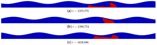
Figure 5.
Single drop shape evolution with time in sinusoidal channel with amplitude during its passage in one corrugated length where the drop undergoes severe topological change due to the variation of channel’s cross-sectional area. All parameters are dimensionless.
Slug flow is now analyzed, and the drop’s shape evolution with time in straight channel with amplitude and initial liquid slug length is presented in Figure 6. As can be noted, the center drop (green color) approaches the front drop (red color) at time , where coalescence takes place. It can also be seen that before drops collision, the center drop elongates and the minimum liquid film thickness becomes larger if compared to time . Such a behavior is due to the increase of drop’s velocity as result of lower pressure behind the front drop. The same physical process was also seen when the initial slug length s is smaller, i.e., . However, the due to the smaller initial distance of the initial slug, the coalescence time is shorter; therefore, for , the following coalescence times were computed: , respectively. The drop shapes of the rear and front drops remained fairly constant during the simulations.
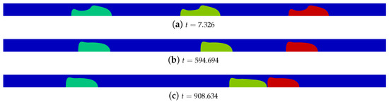
Figure 6.
Drops shape evolution with time in straight channel with amplitude and initial liquid slug length . The rear drop is green color, the center drop is yellow and the front drop is red. The center drop is hydrodynamically affected by the presence of the front and rear drops, thus simulating a complex slug flow. Drop’s coalescence is noted between the front and center drops in time . All parameters are dimensionless.
A slug flow is analyzed in a corrugated channel with amplitude , and the drop’s shape evolution with time is presented in Figure 7 for the initial liquid slug length . The center drop (green color) approaches the front drop (red color) at time , where coalescence takes place, which is faster than the straight channel with same initial conditions. The same physical process was also seen when the initial slug length s was smaller, i.e., . As seen in the straight channel, due to the smaller initial distance of the initial slug, the coalescence time is shorter, therefore for the following coalescence time were computed respectively. The drop shapes of the rear and front drops presented fairly the same dynamical shape of the single drop in sinusoidal channel of Figure 5.
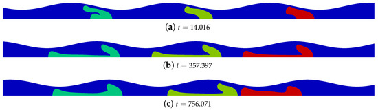
Figure 7.
Drops shape evolution with time in sinusoidal channel with amplitude and initial liquid slug length . The rear drop is green color, the center drop yellow, and the front drop red. The center drop is affected by the presence of the front and rear drops, thus simulating a complex slug flow. Drop coalescence is noted between the front and center drops in time . All parameters are dimensionless.
The evolution of the drop’s rising velocity with time is presented for all test cases simulated in this work in Figure 8. The subplots are divided according to the initial slug length s, and the single drop flow in straight and sinusoidal channels is used as a reference at all plots. As can be seen, the smaller is the initial slug length s, the faster the coalescence takes place, thus resulting in topological change of the two front drops. The drops flow in sinusoidal presented same wavy pattern of velocity variation with time to all test cases. The full lines were used to represent the drop velocity of single drop in straight channel (red color) and sinusoidal (blue color) and the others line types were used for the slug flows in both channels.
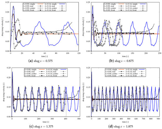
Figure 8.
Center of mass rising velocity as function of time for drops in channels with amplitudes (straight channel, red color) and (sinusoidal, blue color). The figures stand for different drop’s distance compared to single drop simulations with initial liquid slug length: (a) , (b) , (c) , and (d) . All parameters are dimensionless.
Two more interesting results are presented in Figure 9 for initial slug length , where the variation of the ratio of the drop’s perimeter relative to its initial perimeter is investigated in two corrugated lengths in Figure 9a, and the minimum film thickness evolution is presented for two corrugated lengths in Figure 9b. As reference, the single drop flow in the straight channel (red color) and the sinusoidal channel (blue color) is plotted against the slug flow in sinusoidal channel. As can be noted, the drop’s perimeter ratio of the slug flow differs to that of the single drop flow (blue color) when the liquid film thickness hits its maximum length; however, its evolution returns to the same behavior of the single drop flow. On the other hand, the liquid film thickness in the slug flow do not present significant variations if compared to the single drop flow in sinusoidal channel; however, it can be noted that the sinusoidal channel geometry reduces considerably the mean liquid film thickness when compared to the single drop in straight channel (red color).
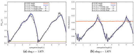
Figure 9.
Single and multiple drops flow in channels with amplitudes (straight channel, red color) and (sinusoidal, blue color) in two corrugated lengths for (a) change in drop’s perimeter ratio relative to its initial perimeter and (b) film thickness evolution. The figures stand for slug flow with drop’s initial slug lengths of . All parameters are dimensionless.
The axisymmetric streamlines are plotted along with the velocity components and and pressure p in Figure 10a to highlight the wake structure of center and front drop’s before coalescence in slug flow with drop’s initial slug lengths . In Figure 10b,c the velocity components, and , and pressure are interpolated axially between at radius , respectively, showing the variation of drop’s velocity and the pressure drop between the center and front drops.
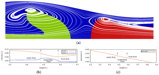
Figure 10.
Wake structure of two consecutive drops before coalescence with drop’s initial slug lengths of . (a) Axisymmetric streamlines of the center and front drops, (b) velocity components and interpolated axially between at radius , and (c) pressure distribution interpolated axially between at radius .
Figure 11 depicts the trend of the coalescence time relative to the initial slug length s for the straight and sinusoidal channels. As can be noted, for initial slug length , the coalescence time increases linearly as s increases. Additionally, as noted previously, the sinusoidal channel anticipates the coalescence time for the same flow parameters of the straight channel.
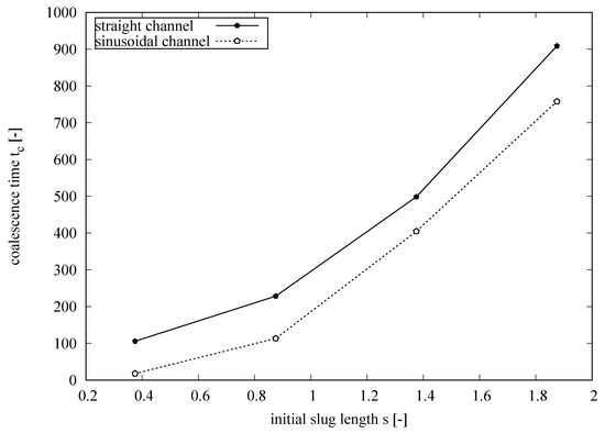
Figure 11.
Trend of the coalescence time relative to the initial slug length s for the straight and sinusoidal channels. For initial slug length , the coalescence time increases linearly as s increases. All parameters are dimensionless.
- Parametric study: wavelength
In the first parametric study, the wavelength has been systematically changed for values while keeping constant the drop’s size factor and all dimensionless numbers used at all simulations for two initial slug lengths . The standard test case for this parametric study is the straight channels with in which the wavelength approaches infinity, where the coalescence time was , respectively, for the initial slug lengths . In the sinusoidal channels, the wavelength parameters presented coalescence time of , respectively, indicating that the coalescence time is not linearly related to the channel’s wavelength as can be seen in Figure 13.
In Figure 12, the final solution before coalescence is shown for all wavelength tested in this parametric study for initial slug length and the respective coalescence time. For the wavelength , no coalescence between the drops took place for time ; therefore, such a wavelength seems to be critical for the simulation parameters used in this work. All the others wavelengths have presented lower coalescence time relative to the straight channel with same parameters.
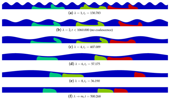
Figure 12.
Slug flow of three consecutive drops in channels with amplitude , drop size factor , wavelength , and initial slug length . For subfigure (e), wavelength in the rear and center drops coalesces in time , while in the others the coalescence takes place between the center and front drops. It is also noted that in subfigure (b) at wavelength no coalescence took place in time .
Figure 13 reveals the coalescence time for the straight and sinusoidal channels relative to the wavelengths. Is is clear that the wavelength is critical for the presented simulation parameters where the coalescence time is much larger than the straight channels with same simulation parameters. On the other hand, all the others wavelengths anticipates the coalescence process when compared to the straight channels.
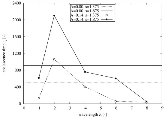
Figure 13.
Trend of the coalescence time relative to the channel’s wavelength for the straight and the sinusoidal channels. It is noted that for wavelength , the coalescence time is higher than the coalescence time for the straight channel with same parameters. The others wavelengths have presented smaller coalescence time. All parameters are dimensionless.
- Parametric study: drop’s size factor
In the last parametric study, the drop size factor is systematically changed for values while keeping constant the channel’s wavelength , initial slug length , and amplitude for the corrugated channel as well as for the straight channel . In Figure 14, the center drop’s perimeter ratio within two corrugated lengths is presented. As expected, the larger is the drop’s size factor , the larger is the perimeter ratio variation.
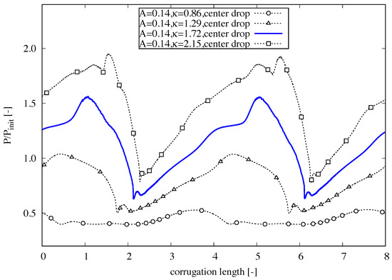
Figure 14.
Center drop’s perimeter ratio within two corrugated lengths for sinusoidal with amplitude , initial slug length and drop size factor for several drops: . As expected, the the larger is the drop’s size factor , the larger is the perimeter ratio variation.
Figure 15 presents a parametric study of coalescence time between drops in slug flow for the sinusoidal channel with amplitude , initial slug length , and several drop’s size factor . For the rear and center drops coalesce, where for the others, the coalescence takes place between the center and front drops. Before coalescence, the drop geometries are similar for and it takes place in the same channel region. The drop’s body increases and the drop’s size factor increases.
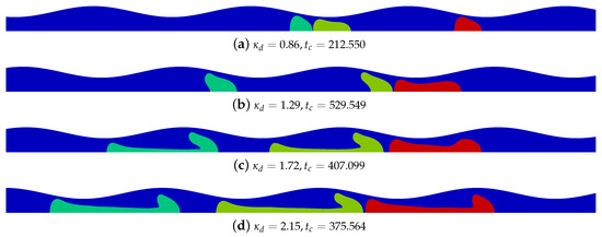
Figure 15.
Parametric study of coalescence time between drops in slug flow for the sinusoidal channel with amplitude , initial slug length and several drop’s size factor . In subfigure (a), the rear and the center drops coalesce, where for the others the coalescence takes place between the center and front drops. All parameters are dimensionless.
Figure 16 shows the trend of the coalescence time relative to the initial slug length s for the sinusoidal channel with amplitude . The drop’s size factor presented larger coalescence time for corrugated channels relative to the straight channels with same parameters. The others drop’s size factors presented smaller coalescence time for the corrugated channel with amplitude relative to the straight channel . Therefore, it is expected to have smaller coalescence time in corrugated channels.
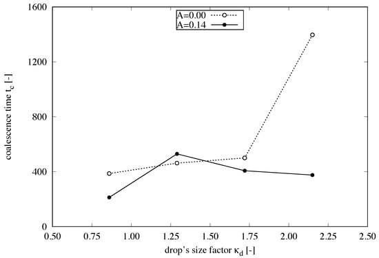
Figure 16.
Trend of the coalescence time relative to the initial slug length s for the sinusoidal channel. The drop’s size factor presented larger coalescence time for corrugated channels relative to the straight channels with same parameters. The others drop’s size factors presented smaller coalescence time for the corrugated channel with amplitude relative to the straight channel . All parameters are dimensionless.
5. Conclusions
In this work, a numerical investigation was carried out to analyze the drop velocity, film thickness, and shape variation for one and three drops in buoyancy-driven motion for diethylene glycol/UCON-1145 (DEG3) two-phase system in straight and sinusoidal channels with dimensionless wavelength and wave amplitude . A state-of-the-art model was employed to accurately compute the dynamics of the drop’s interface motion using a modern moving frame/moving mesh technique within the arbitrary Lagrangian–Eulerian framework which allowed the simulation of very large domains. Several cases with different initial slug lengths s were simulated, and we concluded that the sinusoidal channel anticipates the coalescence of successive drops in slug flows when compared to the straight channel with same flow parameters. Additionally, two parametric studies have been carried out to evaluate drop coalescence time in slug flows varying wavelength and drop size factor . It was observed that the sinusoidal channels with amplitude is likely to decrease the coalescence time relative to the straight channels, except for wavelength and where a different trend has been observed.
Funding
This research was funded by FAPERJ—Foundation for Research Support of the State of Rio de Janeiro.
Conflicts of Interest
The author declares no conflict of interest.
References
- Rush, T.; Newell, T.; Jacobi, A. An experimental study of flow and heat transfer in sinusoidal wavy passages. Int. J. Heat Mass Transf. 1999, 42, 1541–1553. [Google Scholar] [CrossRef]
- Oyakawa, K.; Shinzato, T.; Mabuchi, I. The Effects of the Channel Width on Heat-Transfer Augmentation in a Sinusoidal Wave Channel. JSME Int. J. 1989, 32, 403–410. [Google Scholar] [CrossRef]
- Wang, G.; Vanka, S. Convective heat transfer in periodic wavy passages. Int. J. Heat Mass Transf. 1995, 38, 3219–3230. [Google Scholar] [CrossRef]
- Ničeno, B.; Nobile, E. Numerical analysis of fluid flow and heat transfer in periodic wavy channels. Int. J. Heat Fluid Flow 2001, 22, 156–167. [Google Scholar] [CrossRef]
- Wang, C.C.; Chen, C.K. Forced convection in a wavy-wall channel. Int. J. Heat Mass Transf. 2002, 45, 2587–2595. [Google Scholar] [CrossRef]
- Manavi, S.A.; Ramiar, A.; Ranjbar, A.A. Turbulent forced convection of nanofluid in a wavy channel using two phase model. Heat Mass Transf. 2014, 50, 661–671. [Google Scholar] [CrossRef]
- Anyanwu, I.S.; Hou, Y.; Xi, F.; Wang, X.; Yin, Y.; Du, Q.; Jiao, K. Comparative analysis of two-phase flow in sinusoidal channel of different geometric configurations with application to PEMFC. Int. J. Hydrog. Energy 2019, 44, 13807–13819. [Google Scholar] [CrossRef]
- Su, X.; Yuan, W.; Lu, B.; Zheng, T.; Ke, Y.; Zhuang, Z.; Zhao, Y.; Tang, Y.; Zhang, S. CO2 bubble behaviors and two-phase flow characteristics in single-serpentine sinusoidal corrugated channels of direct methanol fuel cell. J. Power Sources 2020, 450, 227621. [Google Scholar] [CrossRef]
- Muradoglu, M.; Gokaltun, S. Implicit Multigrid Computations of Buoyant Drops Through Sinusoidal Constrictions. J. Appl. Mech. 2005, 71, 857–865. [Google Scholar] [CrossRef]
- Hemmat, M.; Borhan, A. Buoyancy-Driven Motion of Drops and Bubbles in a Periodically Constricted Capillary. Chem. Eng. Commun. 1996, 148–150, 363–384. [Google Scholar] [CrossRef]
- Gros, E.; Anjos, G.R.; Thome, J.R. Interface-fitted moving mesh method for axisymmetric two-phase flow in microchannels. Int. J. Numer. Methods Fluids 2017, 201–217. [Google Scholar] [CrossRef]
- Anjos, G.; Mangiavacchi, N.; Thome, J. An ALE-FE method for two-phase flows with dynamic boundaries. Comput. Methods Appl. Mech. Eng. 2020, 362, 112820. [Google Scholar] [CrossRef]
- Mangiavacchi, N.; Oliveira, G.; Anjos, G.; Thome, J.R. Numerical Simulation of a Periodic Array of Bubbles in a Channel. MecáNica Comput. 2013, XXXII, 1–12. [Google Scholar]
- Balay, S.; Gropp, W.; McInnes, L.; Smith, B. Efficient Management of Parallelism in Object Oriented Numerical Software Libraries. In Modern Software Tools in Scientific Computing; Arge, E., Bruaset, A.M., Langtangen, H.P., Eds.; Birkhäuser Boston: Boston, MA, USA, 1997; pp. 163–202. [Google Scholar]
- Geuzaine, C.; Remacle, J.F. Gmsh: A three-dimensional finite element mesh generator with built-in pre- and post-processing facilities. Int. J. Numer. Methods Eng. 2009, 79, 1309–1331. [Google Scholar] [CrossRef]
- Shewchuk, J.R. Delaunay Refinement Mesh Generation. Ph.D. Thesis, School of Computer Science, Pittsburg, CA, USA, 1997. [Google Scholar]
- Robert, A. A stable numerical integration scheme for the primitive meteorological equations. Atmos. Ocean. 1981, 19, 35–46. [Google Scholar] [CrossRef]
- Pironneau, O. On the transport-diffusion algorithm and its applications to the Navier-Stokes equation. Numer. Math. 1982, 38, 309–332. [Google Scholar] [CrossRef]
- Chorin, A.J. Numerical Solution of the Navier-Stokes Equations. Math. Comput. 1968, 22, 745–762. [Google Scholar] [CrossRef]
- Almatroushi, E.; Borhan, A. Surfactant Effect on the Buoyancy-Driven Motion of Bubbles and Drops in a Tube. Ann. N. Y. Acad. Sci. 2004, 1027, 330–341. [Google Scholar] [CrossRef] [PubMed]
- Hayashi, K.; Kurimoto, R.; Tomiyama, A. Terminal velocity of a Taylor drop in a vertical pipe. Int. J. Multiph. Flow 2011, 37, 241–251. [Google Scholar] [CrossRef]
- Kurimoto, R.; Hayashi, K.; Tomiyama, A. Terminal velocities of clean and fully-contaminated drops in vertical pipes. Int. J. Multiph. Flow 2013, 49, 8–23. [Google Scholar] [CrossRef]
Publisher’s Note: MDPI stays neutral with regard to jurisdictional claims in published maps and institutional affiliations. |
© 2020 by the author. Licensee MDPI, Basel, Switzerland. This article is an open access article distributed under the terms and conditions of the Creative Commons Attribution (CC BY) license (http://creativecommons.org/licenses/by/4.0/).