A Coupled OpenFOAM-WRF Study on Atmosphere-Wake-Ocean Interaction

Abstract

This work aims to better understand how small scale disturbances that are generated at the air-sea interface propagate into the surrounding atmosphere under realistic environmental conditions. To that end, a one-way coupled atmosphere-ocean model is presented, in which predictions of sea surface currents and sea surface temperatures from a microscale ocean model are used as constant boundary conditions in a larger atmospheric model. The coupled model consists of an ocean component implemented while using the open source CFD software OpenFOAM, an atmospheric component solved using the Weather Research and Forecast (WRF) model, and a Python-based utility foamToWRF, which is responsible for mapping field data between the ocean and atmospheric domains. The results are presented for two demonstration cases, which indicate that the proposed coupled model is able to capture the propagation of small scale sea surface disturbances in the atmosphere, although a more thorough study is required in order to properly validate the model.

1. Introduction

Large scale oceanic disturbances, such as earthquakes or tsunamis, are known to generate gravity waves that propagate through the atmosphere up to the ionosphere, where they produce electron density variations that are detectable by global navigation satellite systems (GNSS) [1,2]. Smaller scale disturbances, such as the passage of a surface ship, also clearly manifest in the atmosphere in a number of ways. For example, Yuan et al. [3] trained a deep neural network to detect surface ship tracks that are present in satellite imagery resulting from aerosol-cloud interactions in the atmosphere. Characterizing these types of disturbances and distinguishing them from the normal variability in the ambient environment requires a deep understanding of the dynamics within the atmosphere, ocean, and air-sea interface.

This effort is made all the more challenging, due to the wide range of relevant spatial and temporal scales that are involved in this problem. Characteristic lengths in the atmospheric boundary layer can range from 10 s of meters, in the case of water vapor variability [4,5], to 10 s or 100 s of kilometers, in the case of horizontal rolls and convective cells. On the other hand, the relevant length scales for ship wakes range from <1 m in the vicinity of the ship to 10 s of kilometers behind the vessel, in the case of surface current perturbations. Modeling and simulation solutions exist for the disparate domains, length, and time scales, but a fully coupled solution does not yet exist.

Previous efforts to model the atmosphere-ocean system can be broadly categorized as one-way or two-way coupled. In a one-way coupled model, one model (typically the atmosphere) is used in order to define boundary conditions that drive the response of the other model (typically the ocean). The data are assumed to flow in one direction only, and there is no feedback between the two models. In a two-way model, information passes between the both models during the simulation. The majority of one-way coupled models have primarily focused on initializing microscale CFD analyses with more realistic environmental conditions from mesoscale atmospheric simulations. For example, Boutanios et al. [6] conducted atmospheric mesoscale simulations of the Grosse Isle Manitoba storm whlie using the Weather Research and Forecasting (WRF) model. Boundary conditions that were extracted from this simulation were then used in a microscale CFD analysis in order to investigate the flow around steel transmission towers. Several other authors have taken a similar mesoscale-to-microscale, one-way coupled approach to study the flow around buildings in urban environments [7,8], and around wind farms [9,10,11,12,13,14]. Previous two-way coupled atmosphere-ocean models have largely focused on improved regional and global weather forecasting (e.g., [15,16,17]) and do not possess the necessary spatial resolution in the ocean model in order to resolve small scale disturbances.

This paper presents a one-way coupled atmosphere-ocean model, in which sea surface currents and sea surface temperatures that are predicted by the ocean model are used as boundary conditions for the atmospheric model. This work is distinct from previous works in two ways: (1) atmospheric boundary conditions are set via a microscale CFD ocean model and (2) the CFD ocean model is developed in order to resolve small scale disturbances at the air-sea interface. The remainder of the paper is organized, as follows: Section 2 provides details on the computational approach and discusses some of the limitations of the current coupled model, Section 3 presents results for two demonstration cases that are intended to exercise the one-way coupling approach, and Section 4 provides concluding remarks and a discussion of future work.

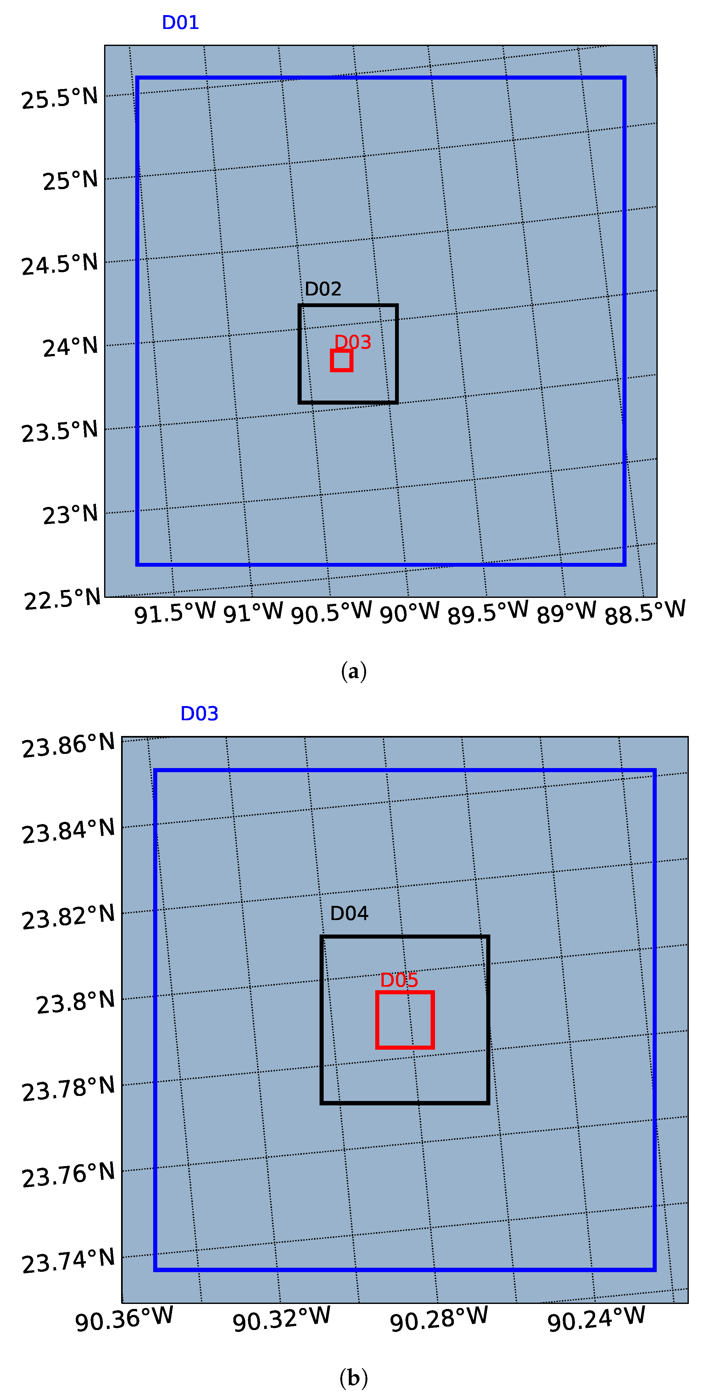
2. Computational Approach

A partitioned approach is used in this work in order to study the coupled problem, in which the atmosphere and ocean domains are solved by separate numerical approaches that are best suited to their different domains. Data (i.e., surface currents, sea surface temperatures, etc.) are exchanged at the air-sea interface via an appropriate coupling scheme. In this case, one-way coupling is accomplished by extracting constant boundary field information from ocean model predictions at the sea surface. Details on each of the component models, as well as the coupling, are provided in the following sections.

2.1. Atmospheric Model

The atmospheric subsystem is solved while using the well-known numerical weather prediction software Weather Research and Forecasting model (WRF). WRF is a fully-compressible, Eulerian non-hydrostatic equations solver that uses terrain-following hydrostatic-pressure vertical coordinates. WRF includes several boundary layer physics schemes and sub-grid scale turbulence formulations. Predictions of three-dimensional winds, pressure, precipitation, air temperature, surface sensible, and latent heat fluxes, as well as many more, are available. WRF is known to be highly scalable and it supports grid nesting to improve resolution over specific areas of interest.

Table 1. A list of the key physics schemes and meteorological data sources that are used in this work.

Atmospheric Model	Configuration
Software	WRF Version 4.2.1
Integration Domain	Gulf of Mexico
Grid	Arakawa semi-staggered C-grid
Initial and boundary conditions	NCEP GDAS/FNL Reanalysis, 0.25${}^{\circ }$ × 0.25${}^{\circ }$
	6-hour update of boundary conditions
SST	NCEP GDAS/FNL Reanalysis
Surface Layer	Revised MM5 Monin-Obukhov scheme [19]
Planetary Boundary Layer	YSU [20]
Microphysics	Thompson scheme [21]
Cumulus	None
Land surface	Noah [22]
Radiation	RRTMG scheme used for longwave and shortwave radiation [23]

provides a summary of the atmospheric model configuration used in the current work. The interested reader is referred to Skamarock et al. [18] for a complete description of WRF.

2.2. Ocean Model

The primary focus of this effort is to characterize the propagation of small scale sea surface perturbations into the atmosphere in realistic environments. To that end, the proposed ocean model is designed in roder to allow for a specification of realistic initial conditions and a variety of geophysical forcings. The equations governing the behavior of the ocean domain are solved while using the open-source CFD software, OpenFOAM™. This work uses OpenFOAM v2006 that is distributed by ESI-OpenCFD (Bracknell, UK).

2.2.1. Governing Equations

The ocean domain is assumed to satisfy the incompressible unsteady Reynolds-averaged Navier–Stokes (URANS) equations for a Boussinesq fluid, such that the balance of mass and momentum can be expressed as

$$\begin{array}{cc}\hfill \nabla ·\mathbf{U}& =0,\hfill \end{array}$$

(1)

$$\begin{array}{cc}\hfill \frac{\partial \mathbf{U}}{\partial t}+\mathbf{U}·\nabla \mathbf{U}-\nu {\nabla }^2\mathbf{U}& =-\nabla \widehat{p}+\nabla ·\overline{u_i^{\prime }{u}_j^{\prime }}-\frac{\Delta \rho }{{\rho }_0}\mathbf{g}+{\mathbf{F}}_{\mathbf{b}}.\hfill \end{array}$$

(2)

Here, $\mathbf{U}={[U,V,W]}^T$ is the mean velocity field, $u_i^{\prime }$ is the fluctuating component of velocity due to turbulence, $\nu$ is the kinematic viscosity, $\Delta \rho =\rho -{\rho }_b\left(z\right)$ indicates a perturbation from the background density profile, ${\rho }_b\left(z\right)$, and ${\rho }_o={\rho }_b(z=0)$ is a reference density. This work also makes use of the piezometric pressure, $\widehat{p}=(p-{\rho }_o\mathbf{g}·\mathbf{x})/{\rho }_o$, where $\mathbf{x}$ is the position vector, $\mathbf{g}$ is the gravity vector, and p is the total pressure. The final term on the right-hand side of Equation (2), ${\mathbf{F}}_{\mathbf{b}}$, represents external body forces other than gravity (e.g., Coriolis force, etc.). Those forcings are neglected in the current work, but they can be easily included in the future.

The evolution of temperature and salinity are directly modeled in this work through the following transport-diffusion equations

$$\begin{array}{cc}\hfill \frac{\partial T}{\partial t}+\nabla ·\left(\mathbf{U}T\right)& =\nabla ·\left({\kappa }_T\nabla T\right)+\nabla ·\overline{u_i^{\prime }{t}^{\prime }},\hfill \end{array}$$

(3)

$$\begin{array}{cc}\hfill \frac{\partial S}{\partial t}+\nabla ·\left(\mathbf{U}S\right)& =\nabla ·\left({\kappa }_S\nabla S\right)+\nabla ·\overline{u_i^{\prime }{s}^{\prime }}.\hfill \end{array}$$

(4)

where $t^{\prime }$ and $s^{\prime }$ are the unsteady fluctuations in temperature, T, and salinity, S, respectively, and ${\kappa }_T$ and ${\kappa }_S$ are the molecular diffusivity of heat and salinity. Modeling temperature and salinity, in this way, allows for the use of realistic environmental profiles that were recorded by oceanic buoys or Regional Ocean Modeling System (ROMS) forecasts. Equations (1)–(4) are closed by an equation of state (EOS) relating pressure, temperature, salinity, and density. In this work, the density is computed while using the TEOS-10 seawater EOS [24].

2.2.2. Turbulence Modeling

A standard $k-ϵ$ model, modified to include buoyancy production effects, is used in order to compute the Reynolds stresses, $\overline{u_i^{\prime }{u}_j^{\prime }}$, and the turbulent fluxes $\overline{u_i^{\prime }{t}^{\prime }}$ and $\overline{u_i^{\prime }{s}^{\prime }}$. The Reynolds stress and turbulent fluxes are given by

$$\begin{array}{cc}\hfill -\overline{u_i^{\prime }{u}_j^{\prime }}& =2{\nu }_t{S}_{ij}-\frac{2}{3}k{\delta }_{ij},\hfill \end{array}$$

(5)

$$\begin{array}{cc}\hfill -\overline{u_i^{\prime }{t}^{\prime }}& =\frac{{\nu }_t}{{\sigma }_T}\frac{\partial T}{\partial x_i},\hfill \end{array}$$

(6)

$$\begin{array}{cc}\hfill -\overline{u_i^{\prime }{s}^{\prime }}& =\frac{{\nu }_t}{{\sigma }_S}\frac{\partial S}{\partial x_i},\hfill \end{array}$$

(7)

where ${\nu }_t=C_{\mu }\frac{k^2}{ϵ}$ is the eddy viscosity and $S_{ij}=\frac{1}{2}\left(\frac{\partial U_i}{\partial x_j}+\frac{\partial U_j}{\partial x_i}\right)$ is the mean rate of strain. The following evolution equations describe the turbulent kinetic energy $k=\frac{1}{2}\left(\overline{u_i^{\prime }{u}_j^{\prime }}\right)$ and dissipation $ϵ$:

$$\begin{array}{cc}\hfill \frac{\partial k}{\partial t}+\nabla ·\left(\mathbf{U}k\right)& =\nabla \left[\left(\nu +\frac{{\nu }_t}{{\sigma }_k}\right)\nabla k\right]+P_k+P_b-ϵ,\hfill \end{array}$$

(8)

$$\begin{array}{cc}\hfill \frac{\partial ϵ}{\partial t}+\nabla ·\left(\mathbf{U}ϵ\right)& =\nabla \left[\left(\nu +\frac{{\nu }_t}{{\sigma }_{ϵ}}\right)\nabla ϵ\right]+C_{1ϵ}\frac{ϵ}{k}(P_k+C_{3ϵ}{P}_b)-C_{2ϵ}\frac{{ϵ}^2}{k},\hfill \end{array}$$

(9)

$$\begin{array}{cc}\hfill P_k& =-\overline{u_i^{\prime }{u}_j^{\prime }}\frac{\partial U_i}{\partial x_j}={\nu }_t{S}^2,\hfill \end{array}$$

(10)

$$\begin{array}{cc}\hfill P_b& ={\rho }^{\prime }\mathbf{g}\frac{{\nu }_t}{P{r}_t}.\hfill \end{array}$$

(11)

Here, $P_k$ is the standard turbulent kinetic energy production term, $P_b$ is the turbulent energy production due to buoyancy effects, and $C_{1ϵ}$, $C_{2ϵ}$, $C_{3ϵ}$, ${\sigma }_k$, and ${\sigma }_{ϵ}$ are the model constants.

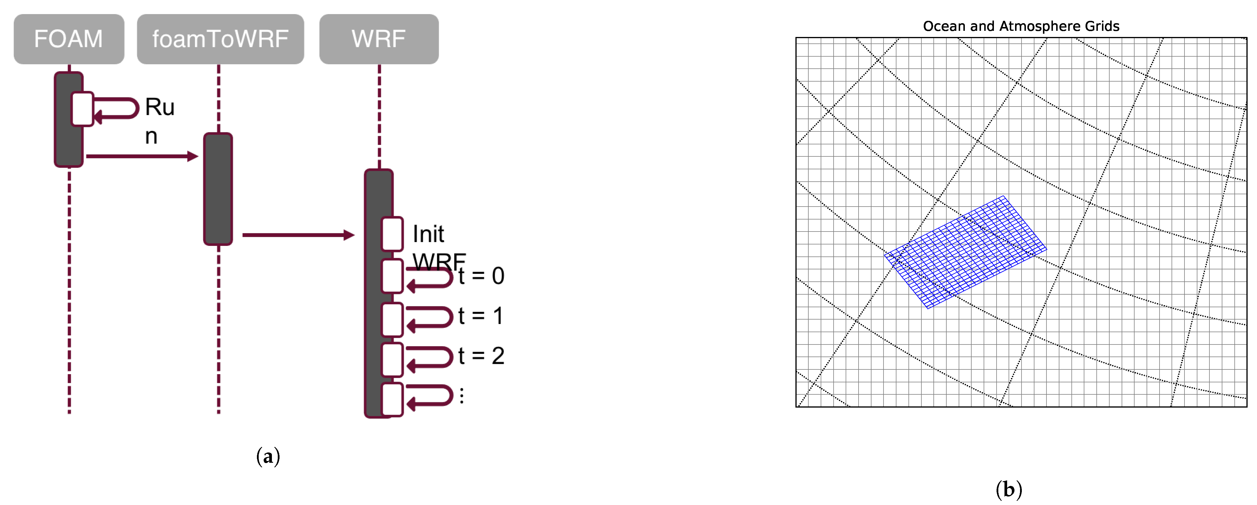
2.3. One-Way Coupling Approach

WRF employs a surface layer scheme that is based on the Revised Monin–Obukhov similarity theory [19]. Within WRF, the surface layer is assumed to be the first vertical layer. Following Varlas et al. [17], the air-sea fluxes of momentum, sensible heat, and latent heat can be expressed as

$$\begin{array}{cc}\hfill \tau & ={\rho }_a{u}_{*}^2={\rho }_a{C}_d{(U-U_s)}^2\hfill \end{array}$$

(12)

$$\begin{array}{cc}\hfill H& =-{\rho }_a{C}_p{u}_{*}{\theta }_{*}={\rho }_a{C}_p{C}_{h}U({\theta }_s-{\theta }_a)\hfill \end{array}$$

(13)

$$\begin{array}{cc}\hfill LH& =L_{\nu }{\rho }_a{u}_{*}{q}_{*}=L_{\nu }{\rho }_a{C}_{q}U(q_s-q_a)\hfill \end{array}$$

(14)

where ${\rho }_a$ is the density of air in the surface layer, $u_{*}$ is the friction velocity, $U_s$, is the sea surface current velocity, and U is the wind speed at the lower layer that is modified by convective velocity and a sub-grid velocity following Beljaars [25] and Mahrt and Sun [26], respectively. Additionally, ${\theta }_{*}$ and $q_{*}$ are the temperature and moisture scales, respectively, $C_p$ is the specific heat capacity at constant pressure, and $L_{\nu }$ is the latent heat of vaporization. ${\theta }_a$ and ${\theta }_s$ are the air and sea surface potential temperatures, respectively, $q_s$ is the specific humidity at the sea surface, $q_a$ is the specific humidity of air at the lower level, and $C_d$, $C_h$, and $C_q$ are the dimensionless bulk transfer coefficients for momentum, sensible heat, and moisture. For details on the parameterization of the bulk transfer coefficients, the reader is referred to Jiménez et al. [19].

In order to couple the atmosphere and ocean domains, predictions for sea surface currents, $U_s,V_s$, and sea surface temperature (SST), ${\theta }_s$, from the ocean model are applied as the bottom surface boundary conditions and used in the surface momentum, heat, and moisture flux calculations of the atmospheric model, as given by Equations (12)–(14). For the results that are presented in this paper, the ocean domain is assumed to evolve much more slowly in time than the atmospheric domain. Consequently, predictions of surface currents and SST from the ocean model are taken to be constant relative to the atmosphere and result in a one-way coupled system. This greatly simplifies the coupling, as no data exchange is required during execution of either the ocean or atmosphere model. Figure 1a illustrates the proposed one-way coupling algorithm and it can be summarized, as follows:

• initialize the ocean and atmospheric models with a consistent ambient environment;
• run the ocean model and extract relevant surface fields ($U_s,V_s,T_s$);
• map surface fields from the ocean domain onto the atmospheric domain;
• overwrite initial atmospheric environment with mapped ocean fields; and,
• run the atmospheric simulation as normal.

2.3.1. Mapping Data Fields

In general, the atmosphere and ocean models will have different domain projections, different resolution requirements, and different reference frames. Consequently, the computational domains will often be mismatched at the air-sea interface, as illustrated in Figure 1b. The process of interpolating sea surface predictions from the ocean model onto the atmospheric domain involves four steps: (1) aligning the atmospheric and ocean domains, (2) transform the atmospheric domain geographic coordinates into Cartesian coordinates, (3) locate the atmospheric points in the ocean domain and interpolate field data from the ocean domain onto the specified interpolation points, and (4) output the new interpolated fields in an appropriate format.

In general, some amount of transformation (rotation and/or translation) is required in order to align the atmospheric and ocean reference frames. Often, the origin of the ocean domain is chosen in such a way as to simplify initialization of the model or to satisfy some other modeling consideration. For example, the surface ship wake application that is presented in Section 3 requires one coordinate (the x-coordinate, in this case) be aligned with the direction of ship motion in order to satisfy the 2D + t assumption. Predictions of sea surface currents must then be transformed in order to align with the ship’s heading relative to the atmospheric domains reference frame.

For the applications under consideration in this work, the computational domain of the ocean model is much smaller than the atmospheric domain. Therefore, it is assumed that the x-coordinate direction is parallel to lines of longitude and the y-coordinate direction is parallel to the lines of latitude. Thus, to a reasonable degree of accuracy, the geographic and Cartesian coordinates can be related via the expressions:

$$\begin{array}{cc}\hfill \mathrm{lat}& =\frac{(y-y_{\min })({\mathrm{lat}}_{\max }-{\mathrm{lat}}_{\min })}{(y_{\max }-y_{\min })}+{\mathrm{lat}}_{\min },\hfill \end{array}$$

(15)

$$\begin{array}{cc}\hfill \mathrm{lon}& =\frac{(x-x_{\min })({\mathrm{lon}}_{\max }-{\mathrm{lon}}_{\min })}{(x_{\max }-x_{\min })}+{\mathrm{lon}}_{\min },\hfill \end{array}$$

(16)

where the min and max subscripts refer domain extents [10].

After the coordinate transformations are complete, the required data field must be interpolated from the ocean domain onto the atmospheric domain. In this work, both linear and cubic two-dimensional (2-D) interpolation schemes were tested. The bi-linear interpolation scheme proved to be the most robust at minimizing errors near domain boundaries and when the resolutions were significantly different between the ocean and atmospheric domains.

Finally, the interpolated boundary data must be stored in a format that is suitable for ingestion in the atmospheric model. In this case, the WRF input files are written in NetCDF format. This step, along with the mapping approach that is described above, has been implemented in a Python-based utility, called foamToWRF. This utility automates the extraction of surface field data from OpenFOAM result files, the alignment of the OpenFOAM and WRF domains, the interpolation of the OpenFOAM data onto the WRF grid, and the export of the resultant bottom boundary conditions in the NetCDF format that is required by WRF. This work uses NetCDF version 4.3.3.1.

3. Results and Discussion

The following section describes two examples of the proposed one-way coupled atmosphere-ocean model. In the first example, the surface currents and SST are analytically generated without the use of an ocean model. In the second example, the ocean model is used in order to predict sea surface current and SST modifications that are caused by the passage of a surface ship. The first example does not use the ocean model and it is intended to demonstrate the ability to modify the WRF boundary conditions, while the second example is illustrative of a more realistic scenario. In both cases, the focus of the investigation is on the microscale Large Eddy Simulation (LES) domain predictions.

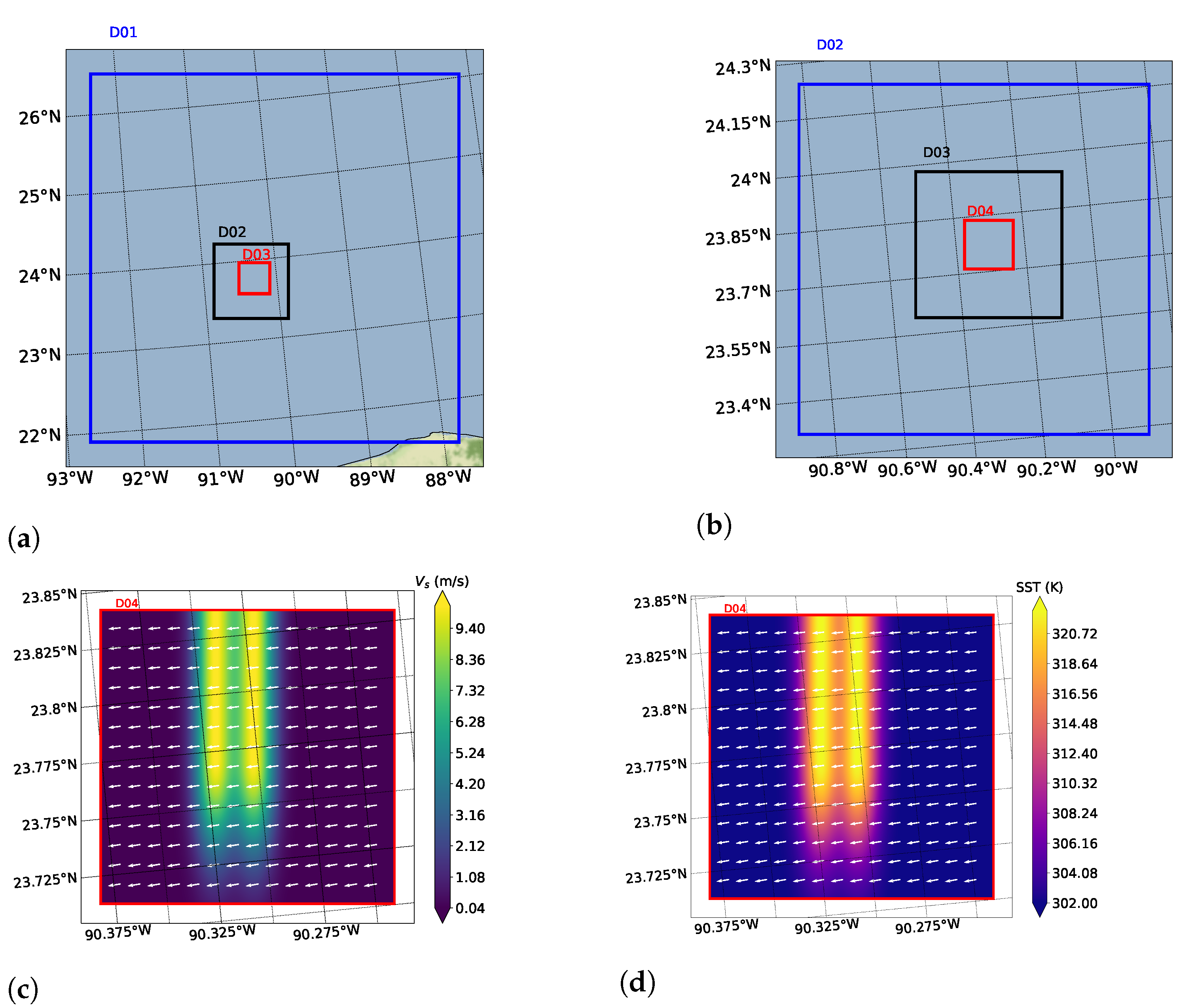
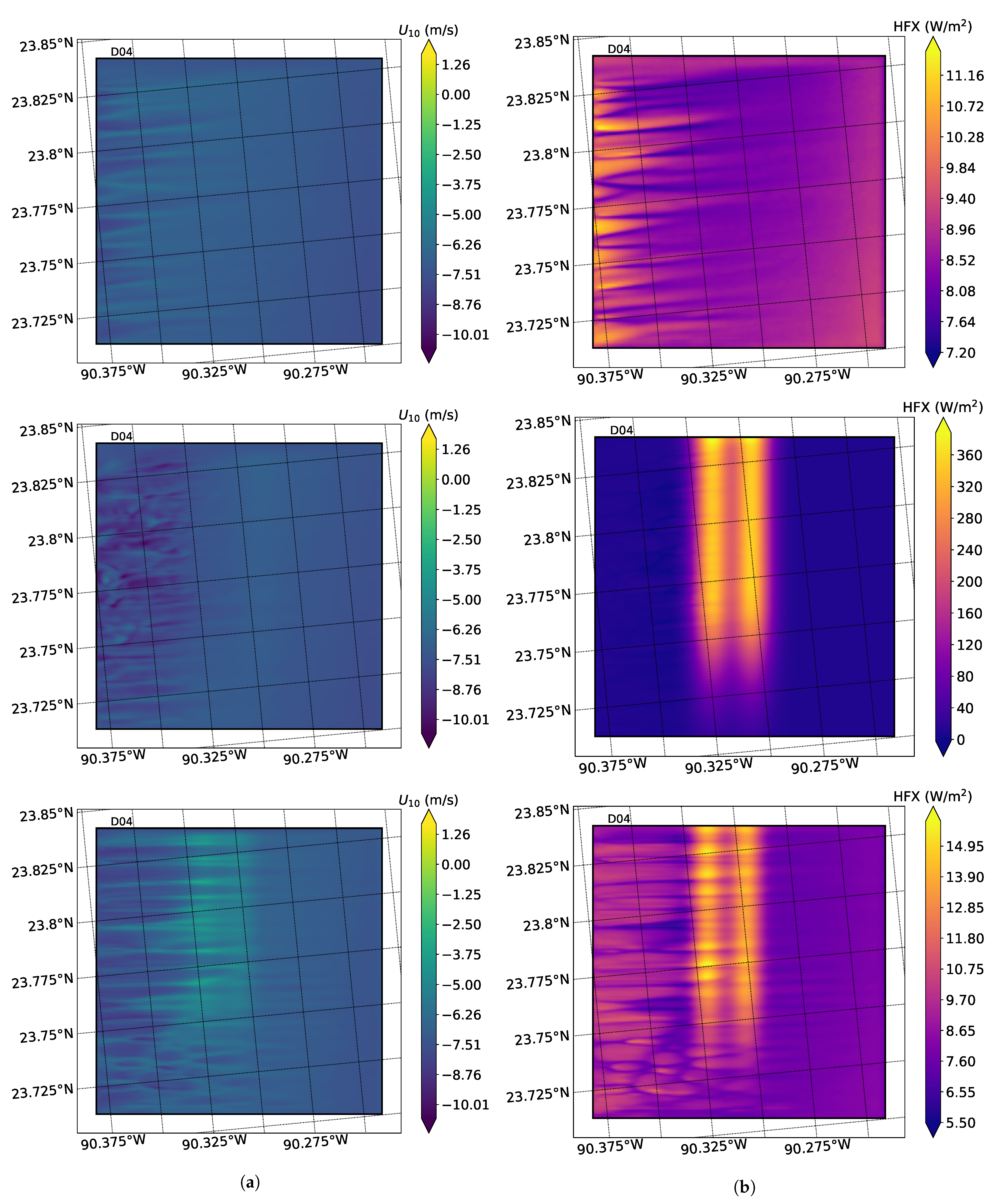
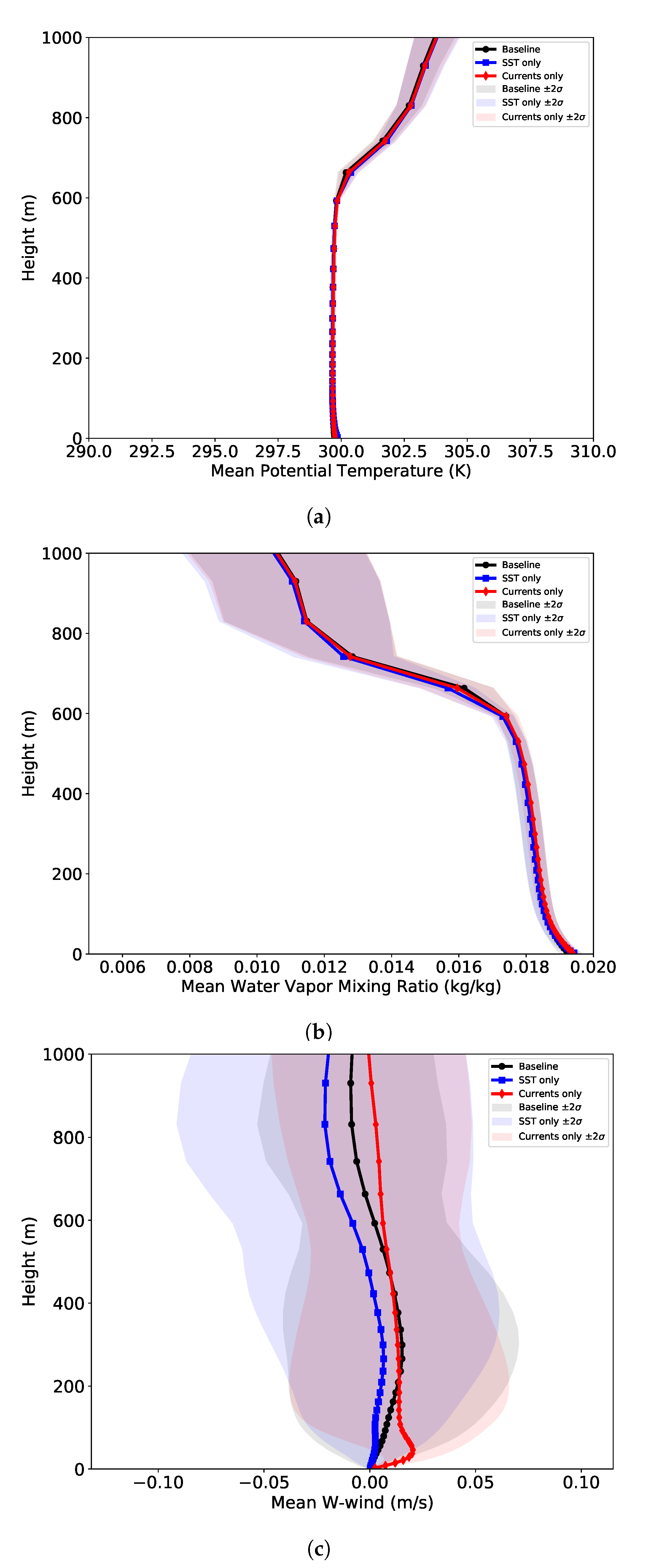
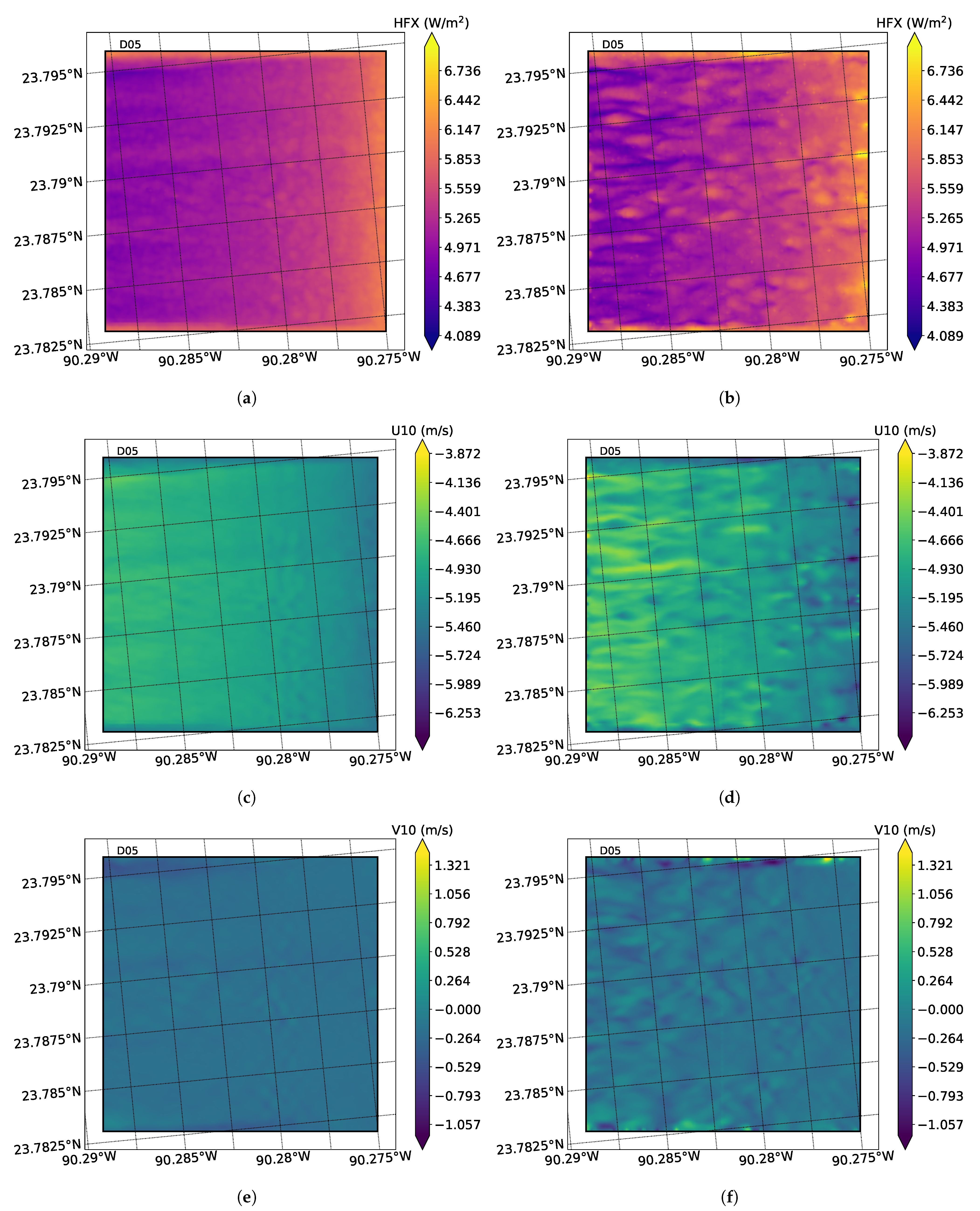
3.1. Application to Surface Jets

This test case was conducted as a demonstration of the one-way coupling process. In this problem, modified sea surface temperatures and currents are analytically described by Gaussian jets to represent an exaggerated surface signature. In this case, two Gaussian jets describe the initial sea surface temperature and sea surface currents:

$$F(x,y)=\sum _i{F}_i(x,y),i=1,2,$$

(17)

where each jet is given by

$$F(x,y)=A\left(x\right)exp\left[-\alpha {(y-y_0)}^2\right],$$

(18)

and

$$A\left(x\right)=A_{0}exp-\beta \left(x\right)x^2.$$

(19)

Here, $\beta \left(x\right)$ is given by

$$\beta \left(x\right)=\left\{\begin{array}{c}0,\mathrm{if}\overline{x}<0\hfill \\ 10,\mathrm{if}\overline{x}>0\hfill \end{array}\right.$$

(20)

where $-\frac{1}{2}\le \overline{x}\le \frac{1}{2}$ is a normalized horizontal location.

Table 2. Gaussian jet parameters that were used in this study.

Parameter	Value for SST	Value for U	Value for V
$A_0$	20 K	0 m/s	10 m/s
$y_{0_1}$	8500 m	-	8500
$y_{0_2}$	6500 m	-	6500
$\alpha$	1× 10${}^{-6}$ m2	-	1 × 10${}^{-6}$ m2

lists the values of the Gaussian jet parameters.

The meteorological environment is chosen, so that surface winds are nearly perpendicular to the direction of the surface currents, as seen in Figure 2b, and the background SST is nearly uniform over the region of interest. This is constructed in such a way as to maximize the induced atmospheric perturbations. NCEP GDAS Final global analysis and forecast data provide meteorological initial and boundary conditions (0.25${}^{\circ }\times$ 0.25${}^{\circ }$ resolution every 6 h). The total simulation length is 10 h, which includes 6 h of spin up time. The overall elevation in the atmospheric domain is approximately 20,500 m, and the simulation utilized a total of four nested grids, which are shown in Figure 2a.

Table 3. The Yonsel University Planetary Boundary Layer scheme (YSU PBL) is used for mesoscale simulations [20].

Simulation Type	PBL Treatment	$\mathbf{\Delta }\mathit{x}$ (m)	Height of 1st Grid Point (m)	Grid Points	$\mathbf{\Delta }\mathit{t}$ (s)
D01 mesoscale	YSU PBL	4500	5	120 × 120 × 81	27.0
D02 mesoscale	YSU PBL	900	5	121 × 121 × 81	5.4
D03 mesoscale	YSU PBL	300	5	151 × 151 × 81	1.8
D04 microscale	LES	100	5	151 × 151 × 81	0.6

lists the details of each grid.

Figure 2c,d show the contours of sea surface zonal currents and SST, respectfully, inside grid D04. As shown, the modified surface fields that are specified in Equations (17)–(20) are completely contained within the most refined grid (D04) in order to avoid introducing spurious behavior at the nested grid boundaries. This is consistent with the WRF published best practice recommendations, which suggest that nested grid boundaries be placed far away from regions of interest [27]. Figure 3 qualitatively shows the impact of the prescribed sea surface modifications, which show contours of the U-component of wind at 10 m elevation and vertical heat flux at the sea surface at the end of the 10-hour simulation time. In this case, three separate simulations are run: (1) a baseline case, in which no modification is introduced to the bottom boundary condition, (2) a SST-only case, in which the the SST is modified, and (3) a current-only case, in which only the meridonal currents are modified. This allows for independent evaluation of each modification on the atmospheric boundary layer. The signature of the prescribed jets is clearly visible in Figure 3, which indicates that the modified boundary conditions are being correctly ingested by the atmospheric model. However, both the 10 m wind and vertical heat flux are prognostic quantities that are computed directly from the imposed boundary conditions and are not necessarily indicative of the sensitivity of the model to the perturbations at the air-sea interface.

Figure 4 provides a more quantitative comparison, which show mean vertical profiles of potential temperature, water vapor mixing ratio, and vertical wind velocity evaluated at the center of grid D04. Again, deviations from the baseline predictions are readily apparent. Potential temperature and water vapor mixing ratio appear to be relatively insensitive to the imposed perturbations over the elevation ranges of interest. On the other hand, the vertical wind velocity that is shown in Figure 4c appears to be much more sensitive to modifications of the air-sea interface, which suggests that vertical wind measurements may be a key indicator in detecting sea surface perturbations in the atmosphere. However, a more rigorous parameter study is required before firm conclusions can be drawn.

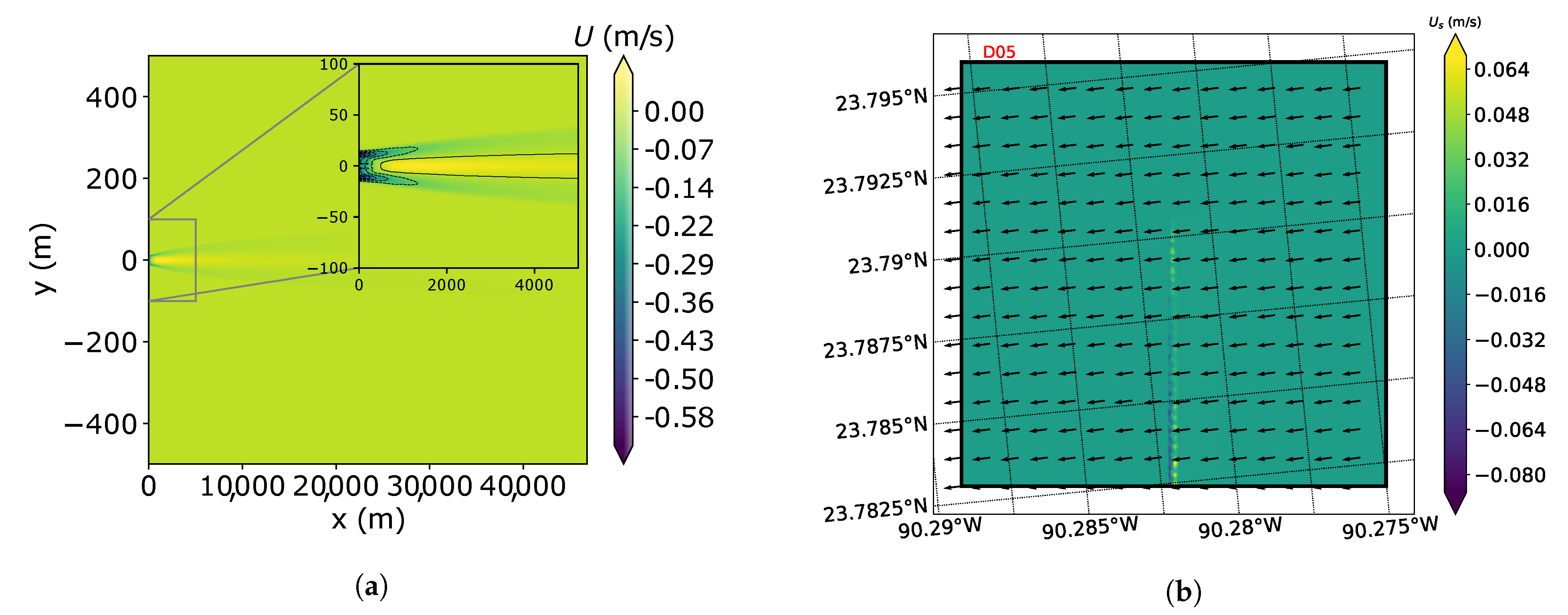
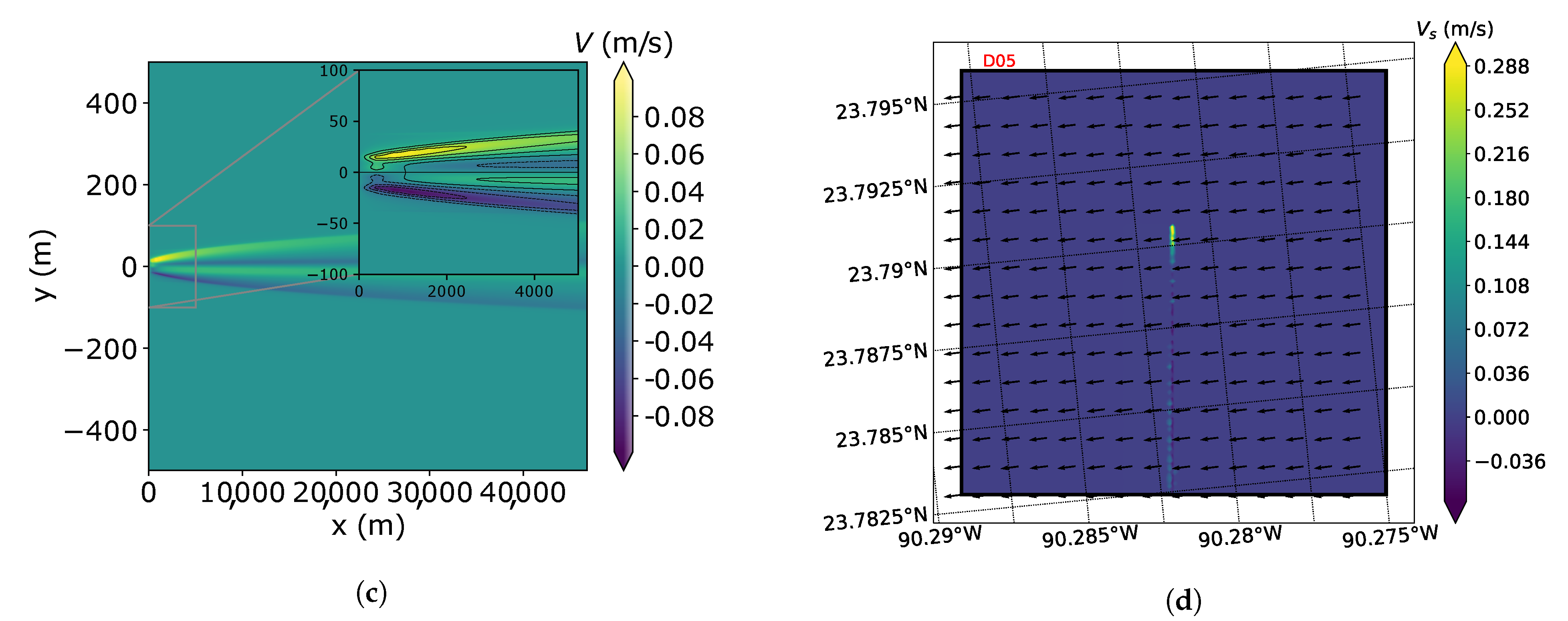
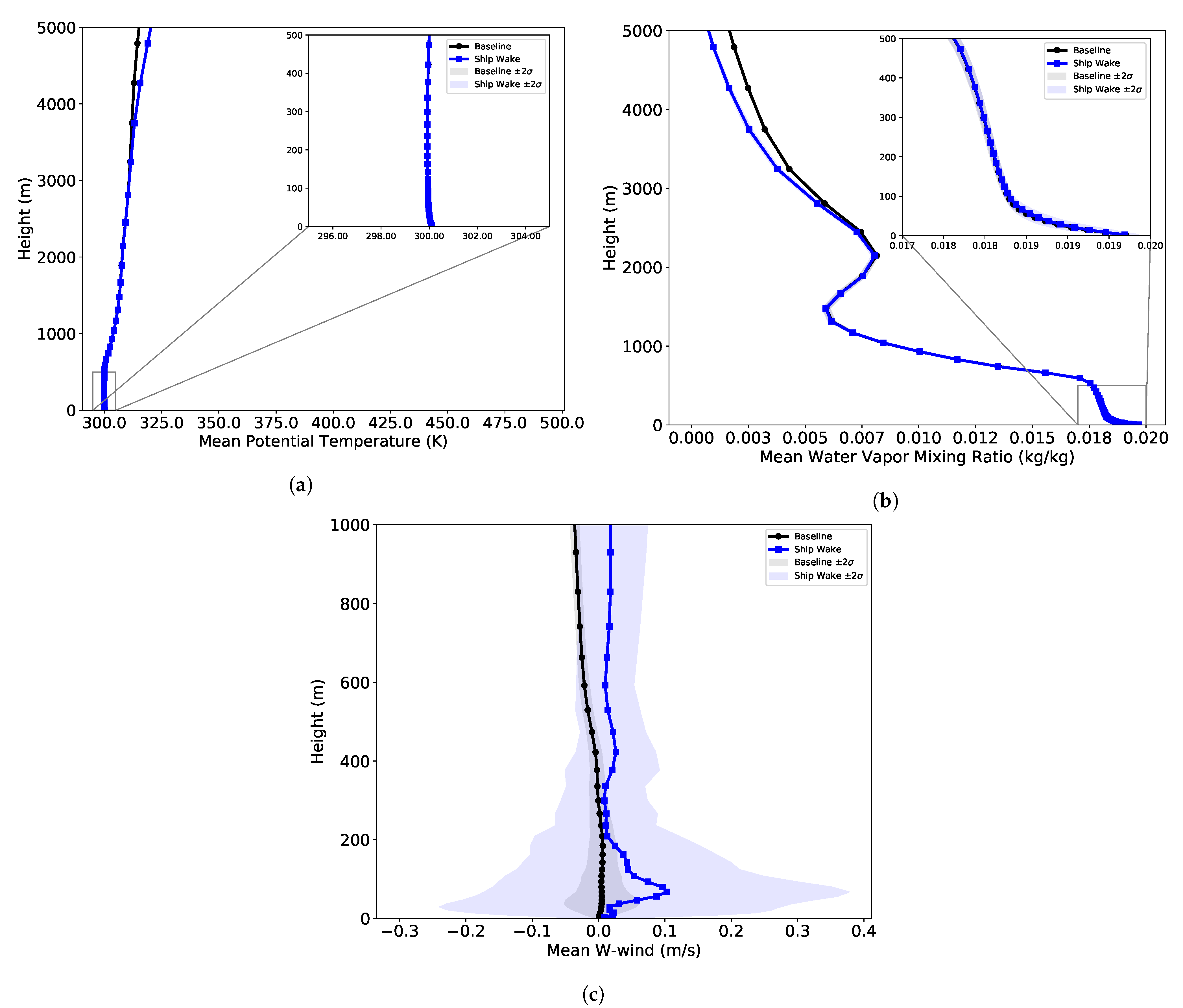
3.2. Application to Surface Ship Wake

This section considers sea surface disturbances due to the passage of a surface ship. As the ship moves through the ocean, it generates a wake that perturbs the sea surface for many kilometers behind the traveling vessel. These perturbations propagate into the atmospheric boundary layer, although to what extent is not yet well understood.

A full, unsteady, three-dimensional simulation of the evolution of a ship wake is not computationally tractable, because of the range of length and time scales that are needed to resolve all of the relevant physics. Instead, a “two-dimensions plus time” (2D + t) approach is used, in which the problem domain is reduced to two spatial dimensions under the assumption that changes in the axial direction are negligible. Under this assumption, the wake is evolved in time, t, and in the ($y,z$) plane. Assuming that the ship is moving with constant speed, $U_0$, the x-location in the wake can be determined from the simulation time as $x=U_{0}t$.

The computational domain of the ocean model has the dimensions of −500 m $<y<$ 500 m by −500 m $<z<$ 0 m and a nominal cell size of 0.3 m. The time step size is set to $\Delta t=$ 1 s and the total simulation duration is 1 h. The $x=$ 0 m location is set to be approximately one-half ship length downstream of the stern of the vessel, so as not to violate the 2D $+ t$ assumptions. In this study, the initial conditions at $t=$ 0 s are generated via a semi-empirical formulation that is similar to Miner et al. [28]. Appendix A of Somero et al. [29] procides the complete details on the semi-empirical wake formulation.

Table 4. Surface ship parameters.

Parameter	Value
Forward speed (m/s)	13
Draft (m)	6.16
Beam (m)	18.9
Heading (deg)	5.52

lists the details of the surface ship used in order to generate the initial conditions at $t=$ 0 s. The ship’s heading was specifically chosen to be aligned with the atmospheric domain’s reference frame in order to assess relative resolution requirements of the atmospheric model.

Field data (e.g., currents, temperature, etc.) from the 2D + t predictions are first sampled along the free-surface ($z=$ 0 m) in order to generate the bottom boundary conditions for the atmospheric model. The sampled fields are then mapped onto the atmospheric domain, as described in Section 2.3.1. Figure 5 shows contours of the sampled surface currents predicted by the ocean model and the corresponding mapped currents.

NCEP GDAS Final global analysis and forecast data provide the meteorological initial and lateral boundary conditions, as in Section 3.1. The total simulated time is 1 h and a total of five nested grid is used in this analysis in order to reach a sufficient level of refinement in the atmospheric domain in order to resolve enough of the wake. It should be noted that a simulation time of 1 h does not, in general, provide sufficient “spin up” time for a valid physical state to develop in the WRF model. As a result, specific model predictions during this time period are very likely inaccurate. Despite this limitation, this analysis is still useful for a qualitative assessment of the one-way coupled approach. Figure 6 shows the nested grids.

Table 5. The Yonsel University Planetary Boundary Layer scheme (YSU PBL) is used for mesoscale simulations [20].

Simulation Type	PBL Treatment	$\mathbf{\Delta }\mathit{x}$ (m)	Height of 1st Grid Point (m)	Grid Points	$\mathbf{\Delta }\mathit{t}$ (s)
D01 mesoscale	YSU PBL	2500	5	120 × 120 × 81	13.0
D02 mesoscale	YSU PBL	450	5	121 × 121 × 81	2.6
D03 mesoscale	YSU PBL	90	5	151 × 151 × 81	0.52
D04 microscale	LES	30	5	151 × 151 × 81	0.17
D05 microscale	LES	10	5	151 × 151 × 81	0.06

lists the relevant details for each grid used in this analysis.

Figure 7 shows atmospheric model predictions of 10 m horizontal winds and sea surface vertical heat flux for the case with and without a ship wake. Larger fluctuations are predicted by the atmospheric model across the entire D05 domain for the ship wake case, and evidence of the ship wake is barely discernible in Figure 7f, around 23.79${}^{\circ }$ N, 90.28125${}^{\circ }$ W.

Figure 8 shows the vertical profiles of potential temperature, water vapor mixing ratio, and vertical wind taken from the center of domain D05. Predictions of potential temperature and water vapor mixing ratio are not strongly affected by the presence of the modified surface currents caused by the ship wake, as was observed in Section 3.1. Conversely, differences in vertical wind, as shown in Figure 8c, are observed much higher into the air column, consistent with the results that are presented in Section 3.1. However, it should be noted that the fluctuations in the vertical wind are approximately an order of magnitude greater than those that are observed in Figure 4, due to the influence of transient pressure waves that are present during the spin up time.

4. Summary and Conclusions

A one-way coupled atmosphere-ocean model was presented in order to study the effects of air-sea interface perturbations on the atmospheric boundary layer. A partitioned approach is used in order to solve the coupled problem, in which the atmospheric domain is modeled while using the numerical weather prediction tool WRF, while the ocean domain is modeled using an unsteady RANS finite volume method implemented in OpenFOAM. One-way coupling is achieved by treating ocean model predictions of sea surface currents and sea surface temperature as a constant bottom boundary condition in the atmospheric model.

Two demonstration cases are presented in order to illustrate the performance of the proposed one-way coupled approach. The first case employs analytical functions in order to specify the perturbed currents and temperatures at the sea surface. The second case uses a semi-empirical relationship to describe the initial conditions of a surface ship wake, which is then evolved in time while using the ocean model. Predicted surface fields from the ocean model are extracted and applied as bottom boundary conditions in the atmospheric model. The modified boundary conditions were clearly visible in contours of 10 m U-wind and vertical heat flux predicted by the WRF model. In both demonstration cases, the vertical profiles of temperature and relative humidity that were predicted by the coupled model were relatively unaffected by the modified boundary conditions, while vertical wind velocity predictions were much more sensitive to the disturbed sea surface conditions.

It is important to note that the results that are presented herein should be considered preliminary and more work is required in order to improve and validate the proposed approach. Techniques, such as Digital Filter Initialization (DFI), need to be explored for reducing atmospheric model “spin up” time [30]. A careful grid convergence study needs to be performed in order to assess the impact of mesh resolution on the model predictions and determine appropriate resolution requirements for this application. Additionally, a parametric study should be conducted to assess which atmospheric parameters are the most sensitive to sea surface disturbances. Techniques for differentiating the relevant atmospheric fluctuations from the naturally occurring variability in the ambient environment is another key aspect of this problem that needs to be investigated. Finally, it will be important to assess whether the assumption of constant bottom boundary conditions is appropriate.

References

1. Komjathy, A.; Yang, Y.M.; Meng, X.; Verkhoglyadova, O.; Mannucci, A.J.; Langley, R.B. Review and perspectives: Understanding natural-hazards-generated ionospheric perturbations using GPS measurements and coupled modeling: NATURAL-HAZARDS-CAUSED TEC PERTURBATIONS. Radio Sci. 2016, 51, 951–961. [Google Scholar] [CrossRef]
2. Savastano, G.; Komjathy, A.; Verkhoglyadova, O.; Mazzoni, A.; Crespi, M.; Wei, Y.; Mannucci, A.J. Real-Time Detection of Tsunami Ionospheric Disturbances with a Stand-Alone GNSS Receiver: A Preliminary Feasibility Demonstration. Sci. Rep. 2017, 7, 46607. [Google Scholar] [CrossRef] [PubMed]
3. Yuan, T.; Wang, C.; Song, H.; Platnick, S.; Meyer, K.; Oreopoulos, L. Automatically Finding Ship Tracks to Enable Large-Scale Analysis of Aerosol-Cloud Interactions. Geophys. Res. Lett. 2019, 46, 7726–7733. [Google Scholar] [CrossRef] [Green Version]
4. Cooper, D.; Eichinger, W.; Barr, S.; Cottingame, W.; Hynes, V.; Keller, C.; Lebbda, C.; Poling, D.A. High-Resolution properties of the Equatorial Pacific marine atmospheric boundary layer from lidar and radiosonde observations. J. Atmos. Sci. 1996, 53, 2054–2074. [Google Scholar] [CrossRef] [Green Version]
5. Hagelberg, C.; Cooper, D.; Winter, C.; Eichinger, W. Scale properities of microscale convection in the marine surface layer. J. Geophys. Res. 1998, 103, 16897–16907. [Google Scholar] [CrossRef]
6. Boutanios, Z.; Miller, C.; Hangan, H. Computational Analysis of the Manitoba September 5 1996 Storm: Mesoscale WRF-ARW Simulations Coupled with Microscale OpenFOAM CFD Simulations. In Proceedings of the Fifth International Symposium on Computational Wind Engineering, Chapel Hill, NC, USA, 23–27 May 2010; p. 8. [Google Scholar]
7. Wyszogrodzki, A.A.; Miao, S.; Chen, F. Evaluation of the coupling between mesoscale-WRF and LES-EULAG models for simulating fine-scale urban dispersion. Atmos. Res. 2012, 118, 324–345. [Google Scholar] [CrossRef]
8. Miao, Y.; Liu, S.; Chen, B.; Zhang, B.; Wang, S.; Li, S. Simulating urban flow and dispersion in Beijing by coupling a CFD model with the WRF model. Adv. Atmos. Sci. 2013, 30, 1663–1678. [Google Scholar] [CrossRef]
9. Leblebici, E.; Tuncer, I.H. Coupled Unsteady Openfoam and WRF Solutions for an Accurate Estimation of Wind Energy Potential. In Proceedings of the VII European Congress on Computational Methods in Applied Sciences and Engineering, Crete Island, Greece, 5–10 June 2016; p. 8. [Google Scholar]
10. Leblebici, E.; Tuncer, D.I.H. Development of OpenFOAM—WRF Coupling Methodolgy for Wind Power Production Estimations. In Proceedings of the 4th Symposium on OpenFOAM in Wind Energy, Delft, The Netherlands, 2–4 May 2016; p. 3. [Google Scholar]
11. Haupt, S.E.; Berg, L.; Anderson, A.; Brown, B.; Churchfield, M.; Draxl, C.; Ennis, B.; Feng, Y.; Kosovic, B.; Kotamarthi, R.; et al. First Year Report of the A2e Mesoscale to Microscale Coupling Project; Technical Report; Pacific Northwest National Laboratory: Richland, WA, USA, 2015. [Google Scholar] [CrossRef]
12. Haupt, S.E.; Kotamarthi, R.; Feng, Y.; Mirocha, J.D.; Koo, E.; Linn, R.; Kosovic, B.; Brown, B.; Anderson, A.; Churchfield, M.J.; et al. Second Year Report of the Atmosphere to Electrons Mesoscale to Microscale Coupling Project: Nonstationary Modeling Techniques and Assessment; Technical Report PNNL-26267, 1573811; Pacific Northwest National Laboratory: Richland, WA, USA, 2017. [Google Scholar] [CrossRef]
13. Temel, O.; Bricteux, L.; van Beeck, J. Coupled WRF-OpenFOAM study of wind flow over complex terrain. J. Wind Eng. Ind. Aerodyn. 2018, 174, 152–169. [Google Scholar] [CrossRef]
14. Mughal, M.O.; Lynch, M.; Yu, F.; Sutton, J. Forecasting and verification of winds in an East African complex terrain using coupled mesoscale—And micro-scale models. J. Wind Eng. Ind. Aerodyn. 2018, 176, 13–20. [Google Scholar] [CrossRef]
15. Warner, J.C.; Armstrong, B.; He, R.; Zambon, J.B. Development of a Coupled Ocean–Atmosphere–Wave–Sediment Transport (COAWST) Modeling System. Ocean Model. 2010, 35, 230–244. [Google Scholar] [CrossRef] [Green Version]
16. Samson, G.; Masson, S.; Lengaigne, M.; Keerthi, M.G.; Vialard, J.; Pous, S.; Madec, G.; Jourdain, N.C.; Jullien, S.; Menkes, C.; et al. The NOW regional coupled model: Application to the tropical Indian Ocean climate and tropical cyclone activity. J. Adv. Model. Earth Syst. 2014, 6, 700–722. [Google Scholar] [CrossRef] [Green Version]
17. Varlas, G.; Katsafados, P.; Papadopoulos, A.; Korres, G. Implementation of a two-way coupled atmosphere-ocean wave modeling system for assessing air-sea interaction over the Mediterranean Sea. Atmos. Res. 2018, 208, 201–217. [Google Scholar] [CrossRef]
18. Skamarock, W.C.; Klemp, J.B.; Dudhia, J.; Gill, D.O.; Liu, Z.; Berner, J.; Wang, W.; Powers, J.G.; Duda, M.G.; Barker, D.M.; et al. A Description of the Advanced Research WRF Model Version 4; NCAR Technical Notes NCAR/TN-556+STR; National Center for Atmospheric Research: Boulder, CO, USA, 2019; p. 162. [Google Scholar]
19. Jiménez, P.A.; Dudhia, J.; González-Rouco, J.F.; Navarro, J.; Montávez, J.P.; García-Bustamante, E. A Revised Scheme for the WRF Surface Layer Formulation. Mon. Weather Rev. 2012, 140, 898–918. [Google Scholar] [CrossRef] [Green Version]
20. Hong, S.Y.; Noh, Y.; Dudhia, J. A New Vertical Diffusion Package with an Explicit Treatment of Entrainment Processes. Mon. Weather Rev. 2006, 134, 2318–2341. [Google Scholar] [CrossRef] [Green Version]
21. Thompson, G.; Field, P.R.; Rasmussen, R.M.; Hall, W.D. Explicit Forecasts of Winter Precipitation Using an Improved Bulk Microphysics Scheme. Part II: Implementation of a New Snow Parameterization. Mon. Weather Rev. 2008, 136, 5095–5115. [Google Scholar] [CrossRef]
22. Niu, G.Y.; Yang, Z.L.; Mitchell, K.E.; Chen, F.; Ek, M.B.; Barlage, M.; Kumar, A.; Manning, K.; Niyogi, D.; Rosero, E.; et al. The community Noah land surface model with multiparameterization options (Noah-MP): 1. Model description and evaluation with local-scale measurements. J. Geophys. Res. Atmos. 2011, 116. [Google Scholar] [CrossRef] [Green Version]
23. Iacono, M.J.; Delamere, J.S.; Mlawer, E.J.; Shephard, M.W.; Clough, S.A.; Collins, W.D. Radiative forcing by long-lived greenhouse gases: Calculations with the AER radiative transfer models. J. Geophys. Res. Atmos. 2008, 113. [Google Scholar] [CrossRef]
24. IOC; SCOR; IAPSO. The International Thermodynamic Equation of Seawater—2010: Calculation and Use of Thermodynamic Properties; Intergovernmental Oceanographic Commission, Manuals and Guides No. 56; UNESCO: Paris, France, 2010. [Google Scholar]
25. Beljaars, A.C.M. The parametrization of surface fluxes in large-scale models under free convection. Q. J. R. Meteorol. Soc. 1995, 121, 255–270. [Google Scholar] [CrossRef]
26. Mahrt, L.; Sun, J. The Subgrid Velocity Scale in the Bulk Aerodynamic Relationship for Spatially Averaged Scalar Fluxes. Mon. Weather Rev. 1995, 123, 3032–3041. [Google Scholar] [CrossRef]
27. Werner, K. Nesting in WRF. In Proceedings of the Basic WRF Tutorial, Boulder, CO, USA, 27–31 January 2020. [Google Scholar]
28. Miner, E.W.; Ramberg, S.E.; Swean, T.J. A Method for Approximating the Initial Data Plane for Surface Ship Wake Simulations; Technical Report NRL Memorandum Report 6376; Naval Research Laboratory: Washington, DC, USA, 1988. [Google Scholar]
29. Somero, J.R.; Basovich, A.; Paterson, E.G. Structure and Persistence of Ship Wakes and the Role of Langmuir-Type Circulations. arXiv 2018, arXiv:1807.00441. [Google Scholar] [CrossRef]
30. LYNCH, P.; HUANG, X.Y. Diabatic initialization using recursive filters. Tellus A 1994, 46, 583–597. [Google Scholar] [CrossRef] [Green Version]
Figure 1. (a) Illustration of the one-way coupling algorithm. The ocean model (FOAM) is run prior to the atmospheric model to generate the required bottom boundary conditions. (b) Depiction of the possible disparate meshes that can exist between ocean and atmospheric model components. The ocean domain, drawn in blue, at a finer grid resolution, and not aligned with the underlying atmospheric domain.
Fluids 06 00012 g001
Figure 2. (a) Overview of nested domains D01-D03, (b) overview of nested domains D02–D03, (c) contours of sea surface meridonal currents (Vs) with white arrows showing 10 m wind direction, and (d) contours of sea surface temperature (SST).
Fluids 06 00012 g002
Figure 3. Predicted contours of (a) 10 m U-wind and (b) Upward heat flux. The top row contains predictions for the baseline case, the middle row contains predictions for SST-only modifications, and bottom most row shows predictions for sea surface current-only modifications.
Fluids 06 00012 g003
Figure 4. Mean vertical profiles of (a) potential temperature, (b) water vapor mixing ratio, and (c) vertical wind velocity. Shaded regions represent ±2σ from the mean value.
Fluids 06 00012 g004
Figure 5. (a) U-component of surface currents predicted by the OpenFOAM model, (b) V-component of surface currents predicted by the OpenFOAM model, (c) U-component of surface currents mapped onto WRF domain, and (d) V-component of surface currents mapped onto WRF domain. The black arrows indicate the direction of the wind at 10 m elevation.
Fluids 06 00012 g005aFluids 06 00012 g005b
Figure 6. Overview of the atmospheric domain extents of (a) D01–D03, and (b) D03–D05 used in the surface ship wake analysis
Fluids 06 00012 g006
Figure 7. Predicted contours of upward heat flux (a,b), 10 m U-wind (c,d), and 10 m V-wind (e,f). Baseline case predictions without a ship wake are shown in the left column and the right column shows predictions with the ship wake present.
Fluids 06 00012 g007
Figure 8. Vertical profiles of (a) potential temperature, (b) water vapor mixing ratio, and (c) vertical wind velocity. Shaded regions represent ±2σ from the mean value.
Fluids 06 00012 g008