Dynamic Analysis and Design Optimization of a Drag-Based Vibratory Swimmer

Abstract

Many organisms achieve locomotion via reciprocal motions. This paper presents the dynamic analysis and design optimization of a vibratory swimmer with asymmetric drag forces and fluid added mass. The swimmer consists of a floating body with an oscillatory mass inside. One-dimensional oscillations of the mass cause the body to oscillate with the same frequency as the mass. An asymmetric rigid fin attached to the bottom of the body generates asymmetric hydrodynamic forces, which drive the swimmer either backward or forward on average, depending on the orientation of the fin. The equation of motion of the system is a time-periodic, piecewise-smooth differential equation. We use simulations to determine the hydrodynamic forces acting on the fin and averaging techniques to determine the dynamic response of the swimmer. The analytical results are found to be in good agreement with vibratory swimmer prototype experiments. We found that the average unidirectional speed of the swimmer is optimized if the ratio of the forward and backward drag coefficients is minimized. The analysis presented here can aid in the design and optimization of bio-inspired and biomimetic robotic swimmers. A magnetically controlled microscale vibratory swimmer like the one described here could have applications in targeted drug delivery.

1. Introduction

Vibrations are a characteristic of many physical systems. Many biological and robotic systems are vibration-driven, i.e., they use periodic motions of their limbs, bodies, or links to generate forces for locomotion. Some examples are flying insects and birds, fish, snakes and worms, swimming micro-organisms, swimming robots, and flapping-wing biomimetic air vehicles. Vibrations may also be used for open-loop stabilization or to change the transient response properties of a system, which is called vibrational control [1,2,3]. The vibrational mechanics of smooth dynamical systems is a well-developed research area. But many vibrational systems are only piecewise-smooth. For example, mechanical systems with dry (Coulomb) friction, mechanical systems with aero- or hydrodynamic forces, electrical circuits with switches, mechanical systems with colliding bodies, and biolocomotion systems [4].

Most often, due to the presence of time-periodic inputs, vibrational systems are time-periodic, and hence time-varying systems. In general, dynamic analysis of time-varying systems is more complicated than for time-invariant systems [5]. However, for classes of time-periodic systems one may use the averaging theorem to transform the original time-periodic system into a time-invariant system which represents the averaged dynamics [6,7,8]. According to the averaging theorem, every stable equilibrium point of the averaged dynamics corresponds to a stable periodic orbit of the original, time-periodic system with the same stability properties of the equilibrium point, and which “hovers” in a small neighborhood around that equilibrium point. Averaging techniques are widely used for dynamical analysis of smooth, time-periodic systems. However in [9,10,11], the averaging theorem is also used for vibration analysis of piecewise-smooth, time-periodic systems. Although more complicated, higher order averaging techniques are also available for the analysis of time-periodic systems [12,13].

One application of vibrational mechanics and averaging is for the dynamic analysis of flying and swimming biolocomotion systems and for the analysis, control, and optimization of biomimetic robotic systems. Most of the available robotic swimmers and fliers use actuated tails, fins, wings, or flagella for motion [14,15,16,17]. Design optimization and optimization of kinematic gaits and inputs of these types of swimmers and fliers have been active research areas [18,19,20,21]. For a review of robotic fliers and macro- and micro-size swimmers see [22,23,24,25]. Dynamics, control, and optimization of mobile robots, such as robotic swimmers and fliers, with no actuated members outside of their bodies have also been subjects of vast research recently. This type of robots use internal rotors, internal oscillatory masses, or deformations of their bodies to generate asymmetric fluid or friction forces for motion [26,27,28,29,30,31,32,33].

In this paper we consider the vibrational analysis and design optimization of a drag-based vibratory swimmer. Unlike conventional robotic swimmers, the proposed swimmer does not have any actuated or moving parts on the exterior of its body, which causes its design, fabrication, and maintenance to be simple. The swimmer with mass M consists of a symmetric body which floats on the surface of a fluid, e.g., water. A mass m oscillates inside the body with constant amplitude and frequency. A rigid, thin, inclined plate (fin) is attached to the bottom of the body and is submerged in the fluid. Hydrodynamic forces act on the fin when it moves relative to the fluid. According to the principle of conservation of linear momentum, the swimmer body oscillates in response to the oscillation the mass m with the same frequency, but a different amplitude. Without the inclined fin, the average velocity of the swimmer is zero. By adding the inclined fin and thus breaking the symmetry of the external swimmer geometry, an asymmetric drag force is applied to the system. Due to the asymmetric drag force, the average velocity of the swimmer will not be zero anymore and the swimmer moves in one direction on average with a certain mean velocity. The fin also changes the total mass of the system by adding an asymmetric fluid added mass to the mass of the system.

We performed finite element simulations with COMSOL Multiphysics^® and determined the drag coefficient of an inclined rigid fin attached to a wall and immersed in a fluid, for different values of the fin angle, and established an approximate relationship between the drag coefficient and the fin angle. Using the averaged dynamics of the system and the relationship we found between the drag coefficient and the fin angle, we determine the optimum fin angle for the swimmer to move at maximum average speed. We present a general theorem for design optimization of a class of vibrational systems with asymmetric forces acting on the system. Through experiments, we verified the dynamic model, optimization technique, and finite element simulation results used for analysis. The results show adequate agreement between analytical and experimental design optimization. The idea presented in this paper may be used for the dynamic analysis and design optimization of macro- and microsized robotic swimmers. e.g., for microrobots used for targeted drug delivery. Though the swimmer presented in this paper floats on the fluid surface, the general class of systems analyzed also includes vibratory swimmers which are immersed in a fluid. For microscale swimmers, one may use micro-cantilever beams as the vibratory mass.

This paper is organized as follows. In Section 2.1 we discuss the averaging of a class of mechanical systems with high-frequency inputs. We use the averaging technique described in Section 2.1 to determine the average dynamics of the vibratory swimmer in Section 2.2, after discussing the equations of motion of the swimmer. Section 2.3 presents the design optimization of the vibratory swimmer to maximize its mean velocity. In Section 2.4 we discuss the results from numerical simulations to determine the hydrodynamic forces acting on a rigid, inclined plate submerged in a fluid. Section 3.1 discusses the averaging and design optimization of vibratory boat with both asymmetric drag and asymmetric fluid added mass forces. The swimmer used for experiments and experimental results are presented in Section 3.2. The main results of the research are summarized in Section 4.

2. Materials and Methods

2.1. Averaging of Piecewise-Smooth Systems with High Frequency Inputs

Consider the first order system

$$\dot{\mathit{x}}=\mathit{f}(\mathit{x})+\mathit{u}(t),\mathit{x}(0)={\mathit{x}}_0$$

(1)

where $\mathit{x}$ is the $n\times 1$ state vector, $\mathit{f}(\mathit{x})$ is a vector field containing smooth or piecewise-smooth functions, and $\mathit{u}(t)={\left(u_1(t),\dots ,u_n(t)\right)}^T$ is the input vector. Consider high-frequency, high-amplitude inputs of the form

$$u_i(t)=\omega v_i(\omega t)$$

(2)

where $v_i(t)$ are zero-mean, T-periodic functions, and $\omega$ is the “high” frequency. Substituting inputs of the form (2) into system (1), the dynamic equations of the system are

$$\dot{\mathit{x}}=\mathit{f}(\mathit{x})+\omega \mathit{v}(\omega t),\mathit{x}(0)={\mathit{x}}_0$$

(3)

where $\mathit{v}(t)={\left(v_1(t),\dots ,v_n(t)\right)}^T$. Using the fast-time scale $\tau =\omega t$, Equation (3) transforms into

$$\frac{d\mathit{x}}{d\tau }=ϵ\mathit{f}(\mathit{x})+\mathit{v}(\tau ),\mathit{x}(0)={\mathit{x}}_0$$

(4)

where $ϵ=\frac{1}{\omega }$ is a “small” number.

Consider the transformation

$$\mathit{x}=\mathit{y}+\int \mathit{v}(\tau )d\tau$$

(5)

where $\int \mathit{v}(\tau )d\tau ={\left(\int v_1(\tau )d\tau ,\dots ,\int v_n(\tau )d\tau \right)}^T$. Taking the derivative with respect to $\tau$, (5) becomes

$$\frac{d\mathit{x}}{d\tau }=\frac{d\mathit{y}}{d\tau }+\mathit{v}(\tau ).$$

(6)

Comparing Equations (4) and (6), one concludes that

$$\frac{d\mathit{y}}{d\tau }=ϵ\mathit{g}(\mathit{y},\tau ),\mathit{y}(0)={\mathit{y}}_0$$

(7)

where

$$\mathit{g}(\mathit{y},\tau )=\mathit{f}\left(\mathit{y}+\int \mathit{v}(\tau )d\tau \right).$$

Since the inputs $v_i(\tau )$ are zero-mean, T-periodic functions, $\mathit{g}(\mathit{y},\tau )$ is also T-periodic in its second argument. The initial conditions ${\mathit{y}}_0$ are determined using transformation (5) for $\tau =0$.

System (7) is in the standard averaging form and its averaged dynamics are represented by [6,7]

$$\frac{d\overline{\mathit{y}}}{d\tau }=ϵ\overline{\mathit{g}}(\overline{\mathit{y}}),\overline{\mathit{y}}(0)={\mathit{y}}_0$$

(8)

where

$$\overline{\mathit{g}}(\overline{\mathit{y}})=\frac{1}{T}{\int }_0^T\mathit{g}(\overline{\mathit{y}},\tau )d\tau .$$

Replacing the fast time scale $\tau$ with the slow time scale t, the averaged dynamics (8) can be written in the form

$$\dot{\overline{\mathit{y}}}=\overline{\mathit{g}}(\overline{\mathit{y}}),\overline{\mathit{y}}(0)={\mathit{y}}_0.$$

(9)

According to the averaging theorem, if the averaged dynamics (9) possesses a hyperbolically stable equilibrium point, then the original time-periodic system (7) possesses a hyperbolically stable periodic orbit in an $O(ϵ)$ neighborhood of that equilibrium point. From transformation (5) it is evident that the average values of $\mathit{x}$ and $\mathit{y}$ are equal, i.e., $\overline{\mathit{x}}=\overline{\mathit{y}}$.

2.2. The Vibratory Swimmer: Dynamic Analysis and Averaging

In this section we derive the equation of motion of the proposed vibratory swimmer and determine its averaged dynamics. The vibratory swimmer considered in this paper consists of a symmetric main body floating on the surface of a fluid. A smaller body oscillates back and forth inside the main body. A rigid, inclined fin is attached under the swimmer and is submerged inside the fluid as shown in Figure 1. Here, we ignore the symmetric hydrodynamic forces acting on the main body and only consider the drag force acting on the fin. We also ignore the pitch and plunge motions of the main body and only consider its one-dimensional motion in the horizontal x-direction.

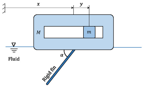
Figure 1. Schematic of the vibratory swimmer consisting of a main body, an oscillating mass m, and a rigid fin attached to the bottom surface of the swimmer at an orientation $\alpha$.

Suppose that the oscillatory mass performs a harmonic oscillation of the form

$$y(t)=\frac{Y}{\omega }cos\omega t$$

(10)

where y is the position vector of the oscillatory mass relative to the main body and $\frac{Y}{\omega }$ and $\omega$ are the amplitude and frequency of its vibrations. The x-component of the linear momentum of the system is

$$P_x=M\dot{x}+m\dot{y}$$

(11)

where M is the total mass of the system including the oscillating mass and the added mass of the fluid, m is the mass of the oscillating body, and x is the position vector of the body. Using Newton’s second law, the equation of motion of the system is

$$M\ddot{x}+m\ddot{y}=-F_D$$

(12)

where $F_D$ is the drag force acting on the system. Replacing $\ddot{y}$ using the expression above, the equation of the system is

$$\ddot{x}=-\frac{F_D}{M}+\frac{mY}{M}\omega cos\omega t,x(0)=x_0,\dot{x}(0)=v_0$$

(13)

In this paper we neglect the symmetric drag force acting on the main body and only consider the drag force of the fin in the form

$$F_D=\frac{1}{2}\rho A{C}_D(\alpha )v^2\mathrm{sgn}(v)$$

(14)

where $\rho$ is the fluid density, A is the fin’s total surface area, $v=\dot{x}$ is the velocity of the main body, $\alpha$ is the fin angle (see Figure 1), and $C_D(\alpha )$ is the drag coefficient of the fin. It is evident that due to the asymmetry of the fin, the drag coefficient $C_D$ and the added mass of the fluid are different in forward ($v>0$) and backward ($v<0$) motion of the swimmer. In this section we consider a symmetric added mass, hence a constant M, and an asymmetric drag coefficient. We discuss the effects of asymmetric added mass in Section 3.1.

Consider the drag coefficient to be

$$C_D(\alpha )=\left\{\begin{array}{ccc}{C}_{D_{\mathrm{p}}}(\alpha )& ;& v>0\\ \frac{1}{2}\left(C_{D_{\mathrm{p}}}(\alpha )+C_{D_{\mathrm{n}}}(\alpha )\right)& ;& v=0\\ C_{D_{\mathrm{n}}}(\alpha )& ;& v<0\end{array}\right.$$

(15)

For simplicity we use $c(\alpha )=\frac{\rho A{C}_D(\alpha )}{2M}$ and $\overline{Y}=\frac{mY}{M}$, and write Equation (13) in the form

$$\dot{v}=-c(\alpha )v^2\mathrm{sgn}(v)+\overline{Y}\omega cos\omega t,v(0)=v_0$$

(16)

where using the drag coefficients $C_{D_{\mathrm{p}}}(\alpha )$ and $C_{D_{\mathrm{n}}}(\alpha )$, the coefficient $c(\alpha )$ is

$$c(\alpha )=\left\{\begin{array}{ccc}{c}_{\mathrm{p}}(\alpha )& ;& v>0\\ \frac{1}{2}\left(c_{\mathrm{p}}(\alpha )+c_{\mathrm{n}}(\alpha )\right)& ;& v=0\\ c_{\mathrm{n}}(\alpha )& ;& v<0\end{array}\right.$$

(17)

The coefficient $c(\alpha )$ can then be written as

$$c(\alpha )=\overline{c}(\alpha )+\tilde{c}(\alpha )\mathrm{sgn}(v)$$

(18)

where

$$\begin{array}{ccc}\hfill \overline{c}(\alpha )& =& \frac{c_{\mathrm{p}}(\alpha )+c_{\mathrm{n}}(\alpha )}{2}\hfill \\ \hfill \tilde{c}(\alpha )& =& \frac{c_{\mathrm{p}}(\alpha )-c_{\mathrm{n}}(\alpha )}{2}.\hfill \end{array}$$

Replacing $c(\alpha )$ in Equation (16) and simplifying, the equation of motion is

$$\dot{v}=-\left(\overline{c}(\alpha )\mathrm{sgn}(v)+\tilde{c}(\alpha )\right)v^2+\overline{Y}\omega cos\omega t,v(0)=v_0,$$

(19)

Equation (19) is in the form of system (3) with $n=1$ and $f(v)=-\left(\overline{c}(\alpha )\mathrm{sgn}(v)+\tilde{c}(\alpha )\right)v^2$, a piecewise-smooth function. Using the fast time scale $\tau =\omega t$ and the transformation

$$v=u+\overline{Y}sin\tau$$

(20)

and following the procedure discussed in Section 2.1, the averaged dynamics of system (19) are determined to be

$$\dot{\overline{u}}=-\frac{\pi \tilde{c}(\alpha )+2\overline{c}(\alpha )\varphi }{\pi M}\left({\overline{u}}^2+\frac{1}{2}{\overline{Y}}^2\right)-\frac{3\overline{c}(\alpha )\overline{Y}cos\varphi }{\pi M}\overline{u},\overline{u}(0)=u_0$$

(21)

where

$$\varphi ={sin}^{-1}\frac{\overline{u}}{\overline{Y}}$$

and the initial condition $u_0=v_0$.

Figure 2 shows time histories of the original, time-periodic system (19) and its averaged dynamics (21). The physical parameters are $M=0.4\mathrm{kg}$, $m=0.2\mathrm{kg}$, $A=0.04{\mathrm{m}}^2$, $\rho =1000{\mathrm{kg}/\mathrm{m}}^3$, $Y=0.2\mathrm{m}/\mathrm{s}$, $\omega =20\mathrm{rad}/\mathrm{s}$, $C_{D_{\mathrm{p}}}=0.1$, and $C_{D_{\mathrm{n}}}=0.2$. The initial conditions are $x_0=0$ and $v_0=0$. By linearizing the averaged dynamics about their equilibrium point ${\overline{u}}_{\mathrm{e}}=0.0135\mathrm{m}/\mathrm{s}$, one can show that this equilibrium point is stable. Therefore the original time-periodic system possesses a stable periodic orbit in a small neighborhood of that equilibrium point.

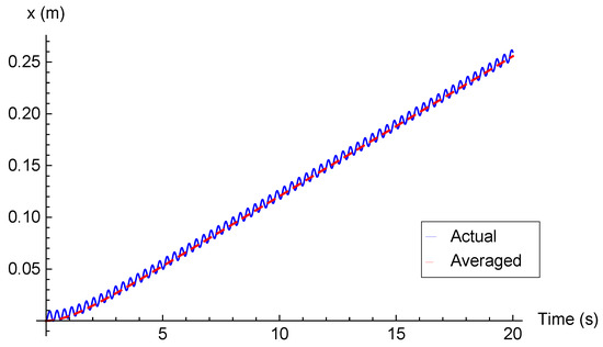
Figure 2. Time histories of the original and averaged systems’ displacements.

2.3. Optimization of a Class of Vibratory Systems

In this section we consider optimization of a class of vibratory systems, including the vibratory swimmer presented in Section 2.2. For the case of the vibratory swimmer, the goal is to determine the fin angle $\alpha$ (see Figure 1) to maximize the average velocity $\overline{v}$ of the main body for a certain set of physical parameters of the system.

Theorem 1.

Consider the first order time-periodic system

$$\dot{x}=-c(p)f(x)+\omega u(\omega t),x(0)=x_0$$

(22)

where $f(x)$ is a smooth or piecewise-smooth function, $u(t)$ is a T-periodic, zero-mean function, $p\in D\subseteq \mathbb{R}$ is a parameter, and

$$c(p)=\left\{\begin{array}{ccc}{c}_{\mathrm{p}}(p)& ;& x>0\\ \frac{1}{2}\left(c_{\mathrm{p}}(p)+c_{\mathrm{n}}(p)\right)& ;& x=0\\ c_{\mathrm{n}}(p)& ;& x<0\end{array}\right.$$

where $c_{\mathrm{p}}(p)$ and $c_{\mathrm{n}}(p)$ are functions of class $C^r$, $r\ge 1$. Suppose that for any value of $p\in D$, the average dynamics of time-periodic system (22) possesses a hyperbolically stable equilibrium point ${\overline{x}}_{\mathrm{e}}={\overline{x}}_{\mathrm{e}}(p)$. Then the extrema of ${\overline{x}}_{\mathrm{e}}$ coincide with the extrema of $\frac{c_{\mathrm{p}}(p)}{c_{\mathrm{n}}(p)}$.

Proof. 

See Appendix A. □

The dynamics (16) of the vibratory swimmer is in the form of (22). Therefore, according to Theorem 1, the average velocity $\overline{v}$ of the main body is maximum if the ratio $\frac{c_{\mathrm{p}}(\alpha )}{c_{\mathrm{n}}(\alpha )}$ is minimum, where $\alpha$ is the fin angle. In this case, while the main body is oscillating back and forth, it also moves forward with maximum speed on average. Therefore the maximum average speed of the swimmer depends on the ratio $\frac{c_{\mathrm{p}}(\alpha )}{c_{\mathrm{n}}(\alpha )}$ of the damping coefficients.

Remark 1.

From system (22) one concludes that if the drag force acting on the rigid fin is proportional to any positive power of the velocity, i.e., $F_D\propto v^r$, $r\in {\mathbb{R}}^{+}$, the average velocity of the swimmer is still maximum if the ratio $\frac{c_{\mathrm{p}}(\alpha )}{c_{\mathrm{n}}(\alpha )}$ is minimum.

2.4. Numerical Simulation of Hydrodynamic Forces Acting on a Rigid, Inclined Fin

In this section we discuss the numerical computation of the drag coefficient of a rigid, rectangular fin immersed in a viscous fluid using COMSOL Multiphysics^® software (The COMSOL Group, Stockholm, Sweden).The fin is attached to an infinite large, fixed surface parallel to the flow, such that the fluid does not flow over the top of the plate. The fin has an angle $\alpha$ with the infinite surface and the flow direction, as shown in Figure 3. The CFD module was used for the computations. No-slip boundary conditions were used at the walls, a constant velocity condition was used at the inlet of the domain, and a pressure boundary condition was used at the exit. Domain size and resolution studies were performed to ensure that the domain size of 14 m × 4 m and CFL number of 1.0 were sufficient to predict a converged value for the drag coefficient.

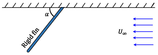
Figure 3. Schematic of the rigid inclined fin immersed in fluid at the bottom of the swimmer.

We used two-dimensional numerical simulations to determine the drag coefficient $C_D$ of the fin for different values of $\alpha \in [0,\pi ]$ rad. To determine the drag coefficient, we divided the total drag force found in the simulations by the dynamic pressure and the fin frontal area. The simulation results were used for design optimization of the vibratory swimmer. Figure 4 presents a snapshot of the simulations for $\alpha ={50}^{\circ }$ after the simulation has reached steady state. The fluid inlet velocity is $U_{\infty }=0.1\mathrm{m}/\mathrm{s}$ and the Reynolds number is $Re=\frac{\rho vL}{\mu }=$ 22,500, where $\rho$ and $\mu$ are the density and dynamic viscosity of the fluid, respectively (assumed to be water at standard pressure and temperature here), and L is the length of the fin, which is $0.3$ m in the simulations, with a thickness of 5 mm. Figure 5 shows the drag coefficient $C_D$ versus the fin angle $\alpha$. For optimization purposes, we approximate the drag coefficient with the following 12^th degree polynomial in terms of $\alpha$, where $\alpha$ is in radians

$$\begin{array}{ccc}\hfill C_D(\alpha )& \approx & 0.018{\alpha }^{12}-0.33{\alpha }^{11}+2.583{\alpha }^{10}-11.48{\alpha }^9+31.74{\alpha }^8-56.38{\alpha }^7\hfill \\ & & +63.98{\alpha }^6-44.5{\alpha }^5+17.31{\alpha }^4-3.766{\alpha }^3+1.44{\alpha }^2+0.132\alpha \hfill \end{array}$$

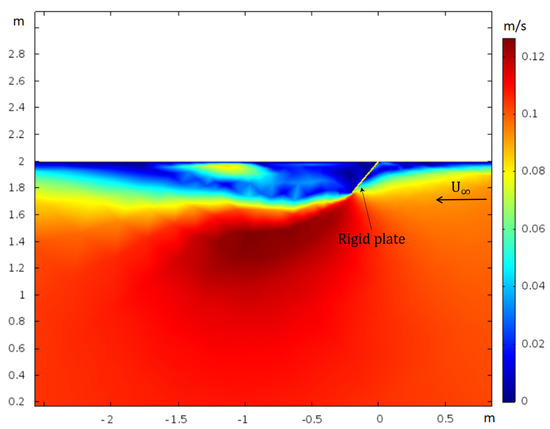
Figure 4. Fluid velocity magnitude for $\alpha ={50}^{\circ }$ and $U_{\infty }=0.1\mathrm{m}/\mathrm{s}$ at steady state, obtained via numerical simulations.

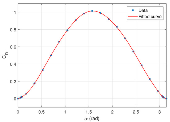
Figure 5. Drag coefficient of the rigid fin versus fin angle, $\alpha$, obtained via numerical simulations.

Using Theorem 1 and the approximate function of $C_D(\alpha )$, one determines the optimum fin angle ${\alpha }_{\mathrm{m}}\approx 9.4^{\circ }$ which generates the maximum average velocity of the swimmer ${\overline{v}}_{\mathrm{m}}\approx 8\mathrm{mm}/\mathrm{s}$, determined using Equation (21). Figure 6 presents the displacement of the swimmer for the three values of fin angle ${\alpha }_1=5^{\circ }$, ${\alpha }_2={\alpha }_{\mathrm{m}}$, and ${\alpha }_3={15}^{\circ }$. Figure 7 shows the average displacement of the swimmer versus time for the parameter values listed in the caption. The rest of the physical parameters are the same as used in simulations to generate Figure 2. It can be seen that though during the transient motion at the beginning of motion the optimum angle ${\alpha }_{\mathrm{m}}$ may not generate the maximum velocity, during steady state motion the swimmer with the optimum angle moves with the maximum speed. Therefore, after a “long enough” time, the swimmer with the optimum fin angle travels farther than the swimmer with any other angle.

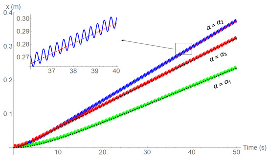
Figure 6. Displacement of the swimmer versus time for ${\alpha }_1=5^{\circ }$, ${\alpha }_2={\alpha }_{\mathrm{m}}={9.4}^{\circ }$, and ${\alpha }_3={15}^{\circ }$. Full: original system, dashed: averaged system.

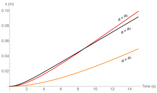
Figure 7. The average displacement of the swimmer versus time for ${\alpha }_1=5^{\circ }$, ${\alpha }_2={\alpha }_{\mathrm{m}}={9.4}^{\circ }$, and ${\alpha }_3={15}^{\circ }$ during transient motion.

3. Results

3.1. The Vibratory Swimmer with an Asymmetric Added Mass

In the vibratory swimmer introduced in Section 2.2 and depicted in Figure 1, the flow of the fluid around the asymmetric inclined fin is not identical during forward ($v>0$) and backward ($v<0$) motions. The asymmetric flow of the fluid in the forward and backward motion of the swimmer generates both asymmetric drag force and asymmetric added mass of the fluid. In this section we discuss the averaging and design optimization of the swimmer when considering realistic asymmetric drag forces and added masses. This is the form of the model that we will compare with experimental results in Section 3.2.

Consider the equation of motion (13) of the system with the total mass of the system $M(\alpha )=M_0+M_{\mathrm{f}}(\alpha )$, where $M_0$ is the mass of the system without considering the fluid added mass, hence it is constant, and $M_{\mathrm{f}}(\alpha )$ is the fluid added mass which depends on the fin angle $\alpha$ and the direction of motion of the swimmer. Therefore, the total mass of the system is

$$M(\alpha )=\left\{\begin{array}{ccc}{M}_{\mathrm{p}}(\alpha )& ;& v>0\\ \frac{1}{2}\left(M_{\mathrm{p}}(\alpha )+M_{\mathrm{n}}(\alpha )\right)& ;& v=0\\ M_{\mathrm{n}}(\alpha )& ;& v<0\end{array}\right.$$

(23)

Defining

$$\begin{array}{ccc}\hfill \overline{M}(\alpha )& =& \frac{M_{\mathrm{p}}(\alpha )+M_{\mathrm{n}}(\alpha )}{2}\hfill \\ \hfill \tilde{M}(\alpha )& =& \frac{M_{\mathrm{p}}(\alpha )-M_{\mathrm{n}}(\alpha )}{2}\hfill \end{array}$$

(24)

the total mass can also be written as $M(\alpha )=\overline{M}(\alpha )+\tilde{M}(\alpha )\mathrm{sgn}(v)$. Defining $a(\alpha )=\frac{1}{2}\rho A{C}_D(\alpha )$, the equation of motion of the system is

$$\begin{array}{c}\dot{x}=v\hfill \\ \dot{v}=-\frac{\overline{a}(\alpha )+\tilde{a}(\alpha )\mathrm{sgn}(v)}{\overline{M}(\alpha )+\tilde{M}(\alpha )\mathrm{sgn}(v)}{v}^2\mathrm{sgn}(v)+\frac{mY}{\overline{M}(\alpha )+\tilde{M}(\alpha )\mathrm{sgn}(v)}\omega cos\omega t\hfill \end{array}$$

(25)

where $\overline{a}(\alpha )$ and $\tilde{a}(\alpha )$ are determined using $a_{\mathrm{p}}(\alpha )=\frac{1}{2}\rho A{C}_{D_{\mathrm{p}}}(\alpha )$ and $a_{\mathrm{n}}(\alpha )=\frac{1}{2}\rho A{C}_{D_{\mathrm{n}}}(\alpha )$ similar to (18). Using the fast-time scale $\tau =\omega t$, Equation (25) can be written as

$$\begin{array}{c}\frac{dx}{d\tau }=ϵv\hfill \\ \frac{dv}{d\tau }=-ϵ\frac{\tilde{a}(\alpha )+\overline{a}(\alpha )\mathrm{sgn}(v)}{\overline{M}(\alpha )+\tilde{M}(\alpha )\mathrm{sgn}(v)}{v}^2+\frac{mY}{\overline{M}(\alpha )+\tilde{M}(\alpha )\mathrm{sgn}(v)}cos\tau \hfill \end{array}$$

(26)

where $ϵ=\frac{1}{\omega }$. Consider the continuous transformation

$$v=\left\{\begin{array}{ccc}u+{\overline{Y}}_{\mathrm{p}}(\alpha )sin\tau & ;& v\ge 0\\ r(\alpha )u+{\overline{Y}}_{\mathrm{n}}(\alpha )sin\tau & ;& v<0\end{array}\right.$$

(27)

where ${\overline{Y}}_{\mathrm{p}}(\alpha )=\frac{mY}{M_{\mathrm{p}}(\alpha )}$, ${\overline{Y}}_{\mathrm{n}}(\alpha )=\frac{mY}{M_{\mathrm{n}}(\alpha )}$, and $r(\alpha )=\frac{M_{\mathrm{p}}(\alpha )}{M_{\mathrm{n}}(\alpha )}=\frac{{\overline{Y}}_{\mathrm{n}}(\alpha )}{{\overline{Y}}_{\mathrm{p}}(\alpha )}$. By taking derivative with respect to $\tau$ from (27) and comparing the result with Equation (26), one gets

$$\frac{dx}{d\tau }=\left\{\begin{array}{ccc}ϵ\left(u+{\overline{Y}}_{\mathrm{p}}(\alpha )sin\tau \right)& ;& v\ge 0\\ ϵ\left(r(\alpha )u+{\overline{Y}}_{\mathrm{n}}(\alpha )sin\tau \right)& ;& v<0\end{array}\right.$$

(28)

$$\frac{du}{d\tau }=\left\{\begin{array}{ccc}-ϵb_{\mathrm{p}}(\alpha )\left(u^2+2{\overline{Y}}_{\mathrm{p}}(\alpha )usin\tau +{\overline{Y}}_{\mathrm{p}}^2(\alpha ){sin}^2\tau \right)& ;& v\ge 0\\ ϵb_{\mathrm{n}}(\alpha )\left(r(\alpha )u^2+2{\overline{Y}}_{\mathrm{n}}(\alpha )usin\tau +\frac{1}{r(\alpha )}{\overline{Y}}_{\mathrm{n}}^2(\alpha ){sin}^2\tau \right)& ;& v<0\end{array}\right.$$

(29)

where $b_{\mathrm{p}}(\alpha )=\frac{a_{\mathrm{p}}(\alpha )}{M_{\mathrm{p}}(\alpha )}$ and $b_{\mathrm{n}}(\alpha )=\frac{a_{\mathrm{n}}(\alpha )}{M_{\mathrm{n}}(\alpha )}$. The time periodic Equations (28) and (29) are in the standard averaging form. Using the averaging theorem, the averaged dynamics of the system is

$$\begin{array}{ccc}\frac{d\overline{x}}{d\tau }& =\hfill & \frac{ϵ}{2\pi }\left({\int }_0^{t_1}\left(\overline{u}+{\overline{Y}}_{\mathrm{p}}(\alpha )sin\tau \right)d\tau +{\int }_{t_1}^{t_2}\left(r(\alpha )\overline{u}+{\overline{Y}}_{\mathrm{n}}(\alpha )sin\tau \right)d\tau +{\int }_{t_2}^{2\pi }\left(\overline{u}+{\overline{Y}}_{\mathrm{p}}(\alpha )sin\tau \right)d\tau \right)\hfill \\ \frac{d\overline{u}}{d\tau }& =\hfill & \frac{ϵ}{2\pi }\left(-{\int }_0^{t_1}{b}_{\mathrm{p}}(\alpha )\left({\overline{u}}^2+2{\overline{Y}}_{\mathrm{p}}(\alpha )\overline{u}sin\tau +{\overline{Y}}_{\mathrm{p}}^2(\alpha ){sin}^2\tau \right)d\tau +{\int }_{t_1}^{t_2}{b}_{\mathrm{n}}(\alpha )(r(\alpha ){\overline{u}}^2+2{\overline{Y}}_{\mathrm{n}}(\alpha )\overline{u}sin\tau \right.\hfill \\ & & \left.+\frac{1}{r(\alpha )}{\overline{Y}}_{\mathrm{n}}^2(\alpha ){sin}^2\tau )d\tau -{\int }_{t_1}^{2\pi }{b}_{\mathrm{p}}(\alpha )\left({\overline{u}}^2+2{\overline{Y}}_{\mathrm{p}}(\alpha )\overline{u}sin\tau +{\overline{Y}}_{\mathrm{p}}^2(\alpha ){sin}^2\tau \right)d\tau \right)\hfill \end{array}$$

(30)

where $t_1=\pi +{sin}^{-1}\frac{\overline{u}}{{\overline{Y}}_{\mathrm{p}}(\alpha )}$ and $t_2=2\pi -{sin}^{-1}\frac{\overline{u}}{{\overline{Y}}_{\mathrm{p}}(\alpha )}$. After some math and replacing the fast-time scale $\tau$ with the slow-time scale t, the averaged dynamics can be written as

$$\begin{array}{cccc}\hfill \overline{v}=& \hfill \dot{\overline{x}}& =& \frac{1}{2\pi }\left(\pi \left(1+r(\alpha )\right)+2\left(1-r(\alpha )\right)\varphi \right)\overline{u}+\frac{1}{\pi }{\overline{Y}}_{\mathrm{p}}(\alpha )\left(1-r(\alpha )\right)cos\varphi \hfill \\ \hfill & \hfill \dot{\overline{u}}& =& -\frac{1}{2\pi }\left(\pi \left(b_{\mathrm{p}}(\alpha )-r(\alpha )b_{\mathrm{n}}(\alpha )\right)+2\left(b_{\mathrm{p}}(\alpha )+r(\alpha )b_{\mathrm{n}}(\alpha )\right)\varphi \right)\left({\overline{u}}^2+\frac{1}{2}{\overline{Y}}_{\mathrm{p}}^2(\alpha )\right)\hfill \\ \hfill & \hfill & & -\frac{3}{2\pi }{\overline{Y}}_{\mathrm{p}}(\alpha )\left(b_{\mathrm{p}}(\alpha )+r(\alpha )b_{\mathrm{n}}(\alpha )\right)\overline{u}cos\varphi \hfill \end{array}$$

(31)

where $\varphi ={sin}^{-1}\frac{\overline{u}}{{\overline{Y}}_{\mathrm{p}}(\alpha )}$.

Knowing the fluid added mass function in terms of the fin angle $\alpha$, i.e., $M_{\mathrm{f}}=M_{\mathrm{f}}(\alpha )$, one can use the averaged dynamics for design optimization of the swimmer, e.g., determine the angle $\alpha$ for maximum speed of the swimmer on average ($\overline{v}$). For this goal, one determines $\alpha$ for: (1) ${\overline{u}}_{\mathrm{e}}$ to be the equilibrium point of the second equation of the averaged dynamics (31), and (2) ${\overline{u}}_{\mathrm{e}}$ maximizes $\overline{v}$. Therefore if ${\overline{u}}_{\mathrm{e}}$ is an equilibrium point of the averaged dynamics, from Equations (31) one can write

$$\begin{array}{ccc}\hfill {\overline{v}}_{\mathrm{e}}& =& F({\overline{u}}_{\mathrm{e}},\alpha )\hfill \end{array}$$

(32)

$$\begin{array}{ccc}\hfill \dot{\overline{u}}{|}_{\overline{u}={\overline{u}}_{\mathrm{e}}}& =& G({\overline{u}}_{\mathrm{e}},\alpha )=0\hfill \end{array}$$

(33)

where $F(\overline{u},\alpha )$ and $G(\overline{u},\alpha )$ are the right hand side of the first and second equations of (31), respectively. Then the problem reduces to a constrained optimization problem; maximize $\overline{v}$ in (32) under constraint (33). Using the method of Lagrange multipliers, we use the function

$$f({\overline{u}}_{\mathrm{e}},\alpha ,\lambda )=F({\overline{u}}_{\mathrm{e}},\alpha )-\lambda G({\overline{u}}_{\mathrm{e}},\alpha )$$

(34)

The equilibrium point ${\overline{u}}_{\mathrm{e}}$ that maximizes or minimizes ${\overline{v}}_{\mathrm{e}}$, and the corresponding angle $\alpha$ are then determined from the following set of equations

$$\begin{array}{cc}\hfill \frac{\partial f}{\partial {\overline{u}}_{\mathrm{e}}}& =0\\ \hfill \frac{\partial f}{\partial \alpha }& =0\\ \hfill \frac{\partial f}{\partial \lambda }& =0\end{array}$$

(35)

Since the determination of the fluid added mass is complicated and outside the scope of this paper, in order to show the effectiveness of the averaging and optimization results in this section, we use a hypothetical added mass and write the total mass of the system in the form

$$M(\alpha )=M_0+0.1\alpha sin\alpha$$

(36)

where $\alpha$ is in radians. Using $M_0=0.4\mathrm{kg}$, the total mass M of the system in terms of $\alpha$ is presented in Figure 8. With the rest of the physical parameters being the same as in Section 2.4, using Equations (35) and (31), one determines the optimum angle ${\alpha }_{\mathrm{m}}\approx 8.7^{\circ }$ and the maximum average velocity of the swimmer ${\overline{v}}_{\mathrm{m}}\approx 0.67\mathrm{cm}/\mathrm{s}$, respectively. The simulation results using three fin angles ${\alpha }_1=5^{\circ }$, ${\alpha }_2={\alpha }_{\mathrm{m}}$, and ${\alpha }_3={13}^{\circ }$ and zero initial conditions are shown in Figure 9.

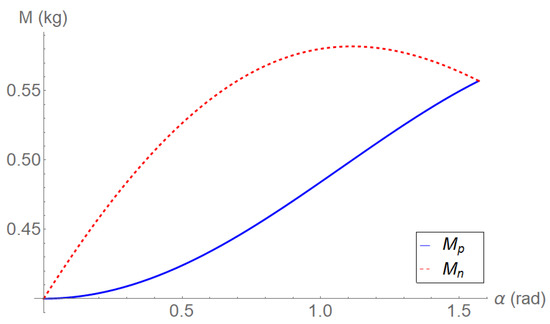
Figure 8. The asymmetric total mass of the swimmer versus the fin angle $\alpha$ for forward motion ($M_p$) and backward motion ($M_n$).

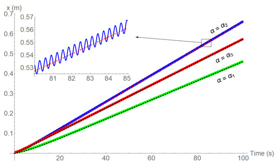
Figure 9. Displacement of the swimmer versus time with an asymmetric added mass for ${\alpha }_1=5^{\circ }$, ${\alpha }_2={\alpha }_{\mathrm{m}}={8.7}^{\circ }$, and ${\alpha }_3={13}^{\circ }$. Full: original system, dashed: averaged system.

3.2. Experiments

To validate the theoretical and numerical results presented in previous sections, we performed experiments with a prototype vibratory swimmer. Here, we describe the device we used in the experiments and present the experimental results. The device used for the experiments consists of a small swimmer floating in a water tank, as shown in Figure 10. A rigid rectangular fin with an adjustable angle is attached to the bottom of the swimmer and is submerged in water. A small servomotor in the swimmer moves (vibrates) a mass back and forth, causing the swimmer to move back and forth with the same frequency. A battery is used to power the servomotor. For the main body we used a rectangular piece of polystyrene. The mass of the swimmer is $M=104\mathrm{g}$, the vibratory mass is $m=43\mathrm{g}$, and the rigid fin is $11.5\mathrm{cm}\times 4.5\mathrm{cm}$. The amplitude and frequency of oscillations are $3\mathrm{cm}$ and $2\pi \mathrm{rad}/\mathrm{s}$, respectively. Interested readers can watch Video S1 in the Supplementary Materials to see the prototype swimmer in operation.

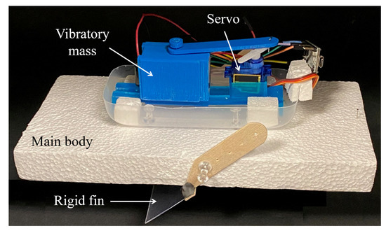
Figure 10. The vibratory swimmer used in experiments.

To perform an experiment, we chose a test fin angle, started the system with zero initial speed, and measured the time required for the swimmer to travel a certain rectilinear distance. This determined the swimmer’s average velocity corresponding to that fin angle. To minimize the effects of disturbances and uncertainties, we repeated the experiment at least five times for each fin angle. We also chose the maximum distance from the starting point possible as a stopping point for the experiments. Figure 11 shows the experimental average swimming versus fin angle compared with the average swimming speed predicted by the theoretical model from Section 3.1. Though the theoretical results predict the maximum average velocity happens for an optimal fin angle of ${\alpha }_{\mathrm{m}}\approx {10}^{\circ }$, the experiments show that the true optimal angle is ${\alpha }_{\mathrm{m}}\approx {20}^{\circ }$. Since the real flow is three-dimensional while the modeled flow used in numerical simulations for determining the drag coefficient is two-dimensional, and considering the other effects neglected in the modeling, such as the hydrodynamic forces acting on the main body, the discrepancy displayed between the theoretical and experimental results is not unexpected.

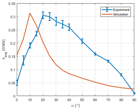
Figure 11. Average speed of the swimmer versus fin angle from experiments and simulations. Although the trends are the same in both cases, including the predicted maximum average swimming speed, which differs by only about $7\%$ between the experiments and theory, the experiments reveal a higher optimal fin angle than that predicted by the two-dimensional theoretical analysis.

From Equation (12) it is evident that the inertial force generated by the acceleration of the sliding mass, i.e., $m\ddot{y}$, causes the back and forth motion of the swimmer. For a swimmer with symmetric drag and added mass, if acceleration of the sliding mass is also symmetric during one cycle, the swimmer does not move on average. However, if the acceleration of the sliding mass, and hence the inertial forces, are not symmetric during one cycle, the swimmer moves in one direction on average. Note that the acceleration can be a zero-mean, periodic function of time, however not symmetric over one cycle. The slider-crank mechanism used in the experiments generates periodic, zero-mean, asymmetric acceleration for the slider. Therefore, even though for the fin angles $\alpha =0$ and $\alpha ={90}^{\circ }$ the drag acting on the system and the added mass are symmetric, the swimmer still possesses non-zero velocity on average. This phenomenon can be clearly seen in Figure 10 for $\alpha =0$ and $\alpha ={90}^{\circ }$.

4. Discussion

In this paper we introduced a mathematical model for a vibratory surface swimmer consisting of a symmetrical body containing an additional vibratory mass inside the body, and an asymmetric rigid fin attached to the bottom of the body and immersed in fluid. Due to the symmetric inertial forces generated by the oscillations of the vibratory mass and the asymmetric hydrodynamic forces acting on the fin, the swimmer moves in one direction on average while performing asymmetric oscillations. Using the averaged dynamics of a class of vibratory systems and constrained optimization, we determined the optimum design for the rigid fin to generate the maximum average speed for the swimmer. The optimum speed predicted by the model and found in the associated physical experiments we performed with a prototype vibratory swimmer different by no more than $7\%$, though the theory predicted an optimal fin angle of around ${10}^{\circ }$ while the actual optimal fin angle was found experimentally to be close to ${20}^{\circ }$.

Generalizing our results beyond the specific parameters and geometries used here, we showed that for a class of vibratory systems with asymmetric damping or drag forces in their forward and backward motions, to maximize or minimize the equilibrium state of the averaged system, one should design the system to maximize or minimize the ratio of the damping or drag coefficients during the forward and backward motion. The class of systems considered in this paper includes both vibratory swimmers moving on a fluid surface (vibratory surface vessels) and vibratory swimmers that are completely submerged in a fluid (vibratory underwater vehicles). The results do not depend on assumptions of swimmer scale or the details of mass oscillation actuation. Therefore the results of this paper can be used for the design optimization of a wide range of underwater vehicles, biomimetic robotic swimmers, and swimming microrobots, including those that could be used for drug delivery.

References

- Meerkov, S.M. Principle of Vibrational Control: Theory and Applications. IEEE Trans. Autom. Control 1980, AC-25, 755–762. [Google Scholar] [CrossRef]
- Bellman, R.E.; Bentsman, J.; Meerkov, S.M. Vibrational Control of Nonlinear Systems: Vibrational Stabilizability. IEEE Trans. Autom.Control 1986, AC-31, 710–716. [Google Scholar] [CrossRef]
- Bellman, R.E.; Bentsman, J.; Meerkov, S.M. Vibrational Control of Nonlinear Systems: Vibrational Controllability and Transient Behavior. IEEE Trans. Autom. Control 1986, AC-31, 717–724. [Google Scholar] [CrossRef]
- Di Bernardo, M.; Budd, C.J.; Champneys, A.R.; Kowalczyk, P. Piecewise-smooth Dynamical Systems; Applied Mathematical Sciences; Springer: London, UK, 2008. [Google Scholar]
- Khalil, H.K. Nonlinear Systems; Prentice-Hall, Inc.: Upper Saddle River, NJ, USA, 1996. [Google Scholar]
- Guckenheimer, J.; Holmes, P. Nonlinear Oscillations, Dynamical Systems, and Bifurcations of Vector Fields; Applied Mathematical Sciences; Springer: New York, NY, USA, 1983. [Google Scholar]
- Sanders, J.A.; Verhulst, F. Averaging Methods in Nonlinear Dynamical Systems; Applied Mathematical Sciences; Springer: New York, NY, USA, 1985. [Google Scholar]
- Bullo, F.; Lewis, A.D. Geometric Control of Mechanical Systems; Texts in Applied Mathematics; Springer: New York, NY, USA, 2005. [Google Scholar]
- Blekhman, I.I. Vibrational Mechanics; World Scientific Publishing Co.: Singapore, 2000. [Google Scholar]
- Thomsen, J.J. Vibrations and Stability; Springer: Berlin, Germay, 2003. [Google Scholar]
- Fidlin, A. Nonlinear Oscillations in Mechanical Engineering; Springer: Heidelberg, Germay, 2006. [Google Scholar]
- Vela, P.A.; Burdick, J.W. Control of underactuated mechanical systems with drift using higher-order averaging theory. In Proceedings of the IEEE Conference on Decision and Control, Maui, HI, USA, 9–12 December 2003; pp. 3111–3117. [Google Scholar]
- Vela, P.A.; Burdick, J.W. A general Averaging Theory via Series Expansions. Am. Control Conf. 2003, 1530–1535. [Google Scholar] [CrossRef]
- Vela, P.A.; Morgansen, K.A.; Burdick, J.W. Underwater locomotion from oscillatory shape deformations. In Proceedings of the IEEE Conference on Decision and Control, Las Vegas, NV, USA, 10–13 December 2002; pp. 2074–2080. [Google Scholar]
- Morgansen, K.A.; Triplett, B.I.; Klein, D.J. Geometric Methods for Modeling and Control of Free-Swimming Fin-Actuated Underwater Vehicles. IEEE Trans. Robot. 2007, 23, 1184–1199. [Google Scholar] [CrossRef]
- Wood, R.J. The First Takeoff of a Biologically Inspired At-Scale Robotic Insect. IEEE Trans. Robot. 2008, 24, 341–347. [Google Scholar] [CrossRef]
- Abbott, J.J.; Peyer, K.E.; Lagomarsino, M.C.; Zhang, L.; Dong, L.; Kaliakatsos, I.K.; Nelson, B.J. How Should Microrobots Swim? Int. J. Robot. Res. 2009, 28, 1434–1447. [Google Scholar] [CrossRef]
- Kelly, S.D.; Murray, R.M. Modeling Efficient Pisciform Swimming for Control. Int. J. Robust Nonlinear Control 2000, 10, 217–241. [Google Scholar] [CrossRef]
- Tahmasian, S.; Allen, D.W.; Woolsey, C.A. On Averaging and Input Optimization of High-Frequency Mechanical Control Systems. J. Vib. Control 2018, 24, 937–955. [Google Scholar] [CrossRef]
- Taha, H.E.; Hajj, M.R.; Nayfeh, A.H. Wing Kinematics Optimization for Hovering Micro Air Vehicles Using Calculus of Variation. J. Aircr. 2013, 50, 610–614. [Google Scholar] [CrossRef]
- Huang, H.; Chao, Q.; Sakar, M.S.; Nelson, B.J. Optimization of Tail Geometry for the Propulsion of Soft Microrobots. IEEE Robot. Autom. Lett. 2017, 2, 727–732. [Google Scholar] [CrossRef]
- Taha, H.E.; Hajj, M.R.; Nayfeh, A.H. Flight dynamics and control of flapping-wing MAVs: A review. Nonlinear Dyn. 2012, 70, 907–939. [Google Scholar] [CrossRef]
- Gerdes, J.W.; Gupta, S.K.; Wilkerson, S.A. A Review of Bird-Inspired Flapping Wing Miniature Air Vehicle Designs. J. Mech. Robot. 2012, 4, 021003. [Google Scholar] [CrossRef]
- Roper, D.T.; Sharma, S.; Sutton, R.; Culverhouse, P. A review of Developments Towards Biologically Inspired Propulsion Systems for Autonomous Underwater Vehicles. Proc. Inst. Mech. Eng. Part M J. Eng. Marit. Environ. 2011, 225, 77–96. [Google Scholar] [CrossRef]
- Diller, E.; Sitti, M. Micro-Scale Mobile Robotics. Found. Trends Robot. 2013, 2, 143–259. [Google Scholar] [CrossRef]
- Ehlers, K.M.; Koiller, J. Micro-swimming Without Flagella: Propulsion by Internal Structures. Regul. Chaotic Dyn. 2011, 16, 623–652. [Google Scholar] [CrossRef]
- Childress, S.; Spagnolie, S.E.; Tokieda, T. A Bug on a Raft: Recoil Locomotion in a Viscous Fluid. J. Fluid Mech. 2011, 669, 527–556. [Google Scholar] [CrossRef]
- Quillen, A.C.; Askari, H.; Kelley, D.H.; Friedmann, T.; Oakes, P.W. A Coin Vibrational Motor Swimming at Low Reynolds Number. Regul. Chaotic Dyn. 2016, 21, 902–917. [Google Scholar] [CrossRef]
- Vetchanin, E.V.; Mamaev, I.S.; Tenenev, V.A. The Self-Propulsion of a Body with Moving Internal Masses in a Viscous Fluid. Regul. Chaotic Dyn. 2013, 18, 100–117. [Google Scholar] [CrossRef]
- Tallapragada, P.; Kelly, S.D. Self-Propulsion of Free Solid Bodies with Internal Rotors via Localized Singular Vortex Shedding in Planar Ideal Fluids. Eur. Phys. J. 2015, 224, 3185–3197. [Google Scholar] [CrossRef]
- Chernous’ko, F.L. The Optimal Periodic Motions of a Two-Mass System in a Resistant Medium. J. Appl. Math. Mech. 2008, 72, 116–125. [Google Scholar] [CrossRef]
- Bolotnik, N.N.; Figurina, T.Y.; Chernous’ko, F.L. Optimal Control of the Rectilinear Motion of a Two-Body System in a Resistive Medium. J. Appl. Math. Mech. 2012, 76, 1–14. [Google Scholar] [CrossRef]
- Chernousko, F.L.; Bolotnik, N.N.; Figurina, T.Y. Optimal Control of Vibrationally Excited Locomotion Systems. Regul. Chaotic Dyn. 2013, 18, 85–99. [Google Scholar] [CrossRef]
- Burns, J.A. Introduction to the Calculus of Variations and Control with Modern Applications; Applied Mathematics and Nonlinear Science Series; Chapman and Hall/CRC: Boca Raton, FL, USA, 2014. [Google Scholar]
© 2020 by the authors. Licensee MDPI, Basel, Switzerland. This article is an open access article distributed under the terms and conditions of the Creative Commons Attribution (CC BY) license (http://creativecommons.org/licenses/by/4.0/).