Aerodynamic Analysis and Design of a Sliding Drag Reduction System Using Graph Neural Networks

Abstract

To maximize competitive performance in motorsports, balancing high downforce for cornering with low drag for straight–line speed is essential. This paper presents the development and optimization of a sliding Drag Reduction System (DRS) integrated with a ducktail guide for a Student Formula racing car. To overcome the computational costs and time constraints of conventional CFD–based iterative design, a Graph Neural Network (GNN) surrogate model was developed to predict aerodynamic coefficients. Unlike traditional models, the GNN directly learns from the geometric graph structure of the multi–element wing, enabling near–instantaneous and highly accurate predictions. CFD results indicated that activating the DRS reduced drag from 82.68 N to 25.51 N, improving the lift–to–drag ratio from 1.67 to 2.67. The GNN surrogate model achieved an R² value exceeding 0.99, demonstrating exceptional predictive fidelity compared to high–resolution simulations. Physical track testing with a Formula SAE vehicle corroborated these findings, showing a 4.6% improvement in 50 m acceleration and a 5.8% increase in maximum speed. This research establishes that GNN–based surrogate models can significantly accelerate the design and optimization of complex variable aerodynamic systems, providing a robust framework for performance enhancement in racing applications.

1. Introduction

When a car is required to achieve maximum speed on a circuit—whether it is a racing car, sports car, or other production vehicle—it is crucial to ensure that the tires maintain firm contact with the ground at all times to maximize acceleration, braking, cornering, and overall performance. At high speeds, the shape of the vehicle generates lift, reducing the load on the tires and lowering the vehicle’s performance limits and stability. To counteract this, aerodynamic devices such as wings are installed to minimize lift by applying downforce to the vehicle body [1], utilizing ground effects [2] on the body or wings [3]. The aerodynamics of two–element wings close to the ground are often studied using CAE analysis, wind tunnel tests, and real–world measurements to verify their effectiveness. Wind tunnel testing with real vehicle geometry is complicated by the presence of a wind tunnel boundary layer [4], which is absent on actual roads, making it difficult to replicate the precise aerodynamic characteristics between the vehicle and the road surface. On–road testing with real vehicles poses challenges as well, as various factors influenced by weather and road conditions are hard to isolate, and geometric modifications are complex and costly. However, CAE analysis has been effective in estimating the aerodynamic forces generated by lift surfaces, complementing wind tunnel testing [5,6,7]. Ahangarnejad et al. investigated integrated vehicle dynamics control with the aim of improving overall vehicle performance, including handling, stability, and comfort, by coordinating four chassis control systems: active aerodynamics control, active rear steering, torque vectoring, and a hydraulically interconnected suspension (HIS) [8]. An isolated full–size rear wing was compared to a 40% scale model of a vintage Indy car [9]. For the performance of single–element front wings with NACA 0015 and 4412 airfoils [10], a comparison between experimental data and computational results showed good agreement when the ground clearance exceeded 0.1 times the chord length. Aero devices offer the advantage of generating downforce but also have the drawback of increasing aerodynamic drag. To address this, a system known as DRS (Drag Reduction System) is used. DRS reduces drag by decreasing the wing’s angle of attack in situations where less downforce is needed, such as when driving at high speeds in a straight line. Formula SAE, a university design competition in which student teams design, build, and race their own open–wheel cars, allows for the use of DRS due to the relatively flexible regulations [11].

One of the key challenges is balancing the rear wing’s downforce with the aerodynamic drag it produces. Several factors influence the aerodynamic characteristics of a rear wing, including the angle of attack (here after AOA), camber, and wing profile. While there are various DRS mechanisms, the most common include systems that temporarily reduce the angle of attack on the upper wings of a multi–element wing, or those that feature an air outlet on the low section of the wing to channel airflow [12]. The primary goal is to reduce drag by deliberately disrupting airflow around the wings—when downforce is less critical at high speeds—and thereby minimizing the wing’s downforce–generating function [13]. Traditional Drag Reduction Systems (DRS) primarily focus on adjusting the Angle of Attack (AOA) of the wing flap. However, the potential for dynamically optimizing the relative spatial positioning between aerodynamic elements—specifically in the longitudinal and vertical directions—has been largely overlooked in relation to varying vehicle speeds.

A ducktail is an aerodynamic device that deflects the rear boot lid of a vehicle upwards. Its primary function is to increase downforce at the rear of the vehicle by creating an air vortex above the boot lid, generating negative pressure that pulls up the airflow beneath the vehicle and increases its velocity. When combined with a rear wing, the ducktail also serves as a wind guide, directing airflow to follow the contours of the wing’s underside. This creates a synergistic effect, improving the efficiency of the rear wing.

The effect of improving vehicle dynamics has been confirmed for the conventional DRS using an independent large rear wing [12]. However, the above–mentioned ducktail has a rectifying effect, and the same level of effect can be expected even if the rear wing is made smaller and lighter. In this study, a sliding DRS mechanism integrated with the vehicle’s body shape was investigated using 3D CAD and CFD analysis. The proposed Sliding DRS (SDR) introduces a multi–dimensional design space where the longitudinal and vertical displacements must be integrated with the AOA. Furthermore, the addition of aerodynamic devices such as a “ducktail” on the vehicle body enhances downforce at low speeds but introduces highly complex, separated flow interactions. This complexity makes the identification of an optimal configuration significantly more challenging. The goal was to significantly reduce drag without a substantial loss of downforce. The effectiveness of this design was verified, and its performance evaluated.

Optimization of aerodynamic performance is a crucial factor determining vehicle competitiveness in motorsports. Specifically, active aerodynamic devices are indispensable for enhancing performance under specific driving conditions. However, finding their optimal actuation conditions and geometries necessitates high–resolution CFD simulations and physical wind tunnel experiments, demanding significant computational resources and time. To resolve this bottleneck, there is a strong need for the development of surrogate models that can accurately approximate the results of CFD analysis. Several studies have already reported on the application of machine learning (ML) to automotive aerodynamic simulations. Bleeker et al. reported on accelerating automotive aerodynamic simulations using deep learning [14]. Dube et al. applied and compared the accuracy of multiple ML techniques, including Kriging and Neural Networks, for predicting vehicle aerodynamic drag, covering the latest trends such as attempts to directly use raw geometry data as input [15]. Furthermore, Bekemeyer et al. conducted a benchmark study to standardize the evaluation of aerodynamic surrogate models, which often include models like Gaussian Process Regression (GPR) and Support Vector Regression (SVR) [16].

High–fidelity CFD simulations entail significant computational costs, posing a major bottleneck in the design optimization process, which requires numerous geometric iterations. To address this challenge, aerodynamic performance prediction methods utilizing machine learning as low–cost surrogate models are rapidly evolving. Within data–driven frameworks, research has predominantly focused on Convolutional Neural Networks (CNNs); for instance, Guo et al. [17] and Thuerey et al. [18] proposed methods to represent airfoil geometries as pixel data or Signed Distance Functions (SDFs) to instantaneously infer flow fields and aerodynamic coefficients via CNNs. Sekar et al. [19] achieved aerodynamic coefficient prediction across a wide range of operating conditions by integrating geometric parameters with CNN–based image information. Furthermore, to overcome the inherent limitations of CNNs in representing geometry through pixels, Kashefi et al. [20] proposed a learning framework utilizing point clouds, enabling flexible predictions for irregular data arrangements. Raissi et al. [21] applied the concept of Physics–Informed Neural Networks (PINNs) to incorporate governing equations and physical symmetries into loss functions, thereby enabling physically plausible C_l and C_d predictions even with sparse training data. Zhang et al. [22] targeted airfoils with Trailing Edge Flaps (TEF) and proposed a high–speed, high–precision prediction method using deep learning that introduces a “multi–task learning” framework in addition to the fusion of geometric information and scalar quantities. Furthermore, significant progress has been observed in both forward and inverse problems, including research on gradient–enhanced surrogate models to optimize the trade–off between computational cost and accuracy [23], and design methods using Generative Adversarial Networks (GANs) for inverse geometry design based on desired aerodynamic characteristics [24]. As techniques for more efficient geometric feature extraction, approaches utilizing Graph Neural Networks (GNNs) and point clouds have gained significant attention. Jacob et al. [25] compared the performance of surrogate models, including GNNs, with traditional CNNs using real–world datasets from external vehicle aerodynamics. However, several issues persist when substituting CFD with machine learning, such as the lack of physical guarantees, the necessity for high–fidelity CFD data, and the difficulty of conditional prediction due to the dimensional imbalance between high–dimensional geometric information and low–dimensional scalar conditions, such as the angle of attack and Reynolds number [20]. Additionally, mesh dependency, the difficulty of uncertainty quantification, and a lack of interpretability remain constraints in engineering applications. Moreover, theoretical limitations in the expressive power of GNNs have been demonstrated, where certain distinct structures may become indistinguishable to the network [26]. Sun et al. [27] pointed out that deep learning models often neglect physical constraints, such as the Navier–Stokes equations, and discussed the efficacy and limitations of incorporating physical terms into loss functions. Kashinath et al. [28] also provided a comprehensive overview of how purely data–driven models, which do not account for physical information, are prone to generating non–physical solutions in fluid analysis. Furthermore, quantitative studies have shown that both standard neural networks [29] and GNNs [30] are highly vulnerable when applied to complex flows involving separation or to Reynolds numbers and geometries that fall outside the range of the training data. Existing research and predictions have largely been limited to single airfoils in uniform flow, making them difficult to apply to complex flows involving multi–element or “ducktail” configurations. The difficulty of extrapolating computational domains has also been identified as a critical challenge. This study addresses the application of a sliding DRS, where the relative positions of multiple wing elements change dynamically, representing an exceptionally high level of complexity in aerodynamic modeling.

In this study, we specifically adopt the Graph Neural Network (GNN) approach. GNN is advantageous because it can continue learning while preserving the structural relationship of the wing’s shape, even when the geometry changes slightly. This enables a more faithful modeling of the transmission of physical influences within a complex DRS, where multiple elements such as intricate wing shapes, multi–element wings, and cowl shapes interact. Given the expanded design space and the non–linear nature of these aerodynamic interactions, relying solely on conventional Computational Fluid Dynamics (CFD) for comprehensive optimization is computationally prohibitive. Therefore, there is a critical need for an efficient surrogate model. Specifically, a Graph Neural Network (GNN) approach is adopted here, as it is uniquely suited to capturing the topological relationships between shifting geometric components, offering a high–fidelity alternative to exhaustive CAE simulations. The objective of this development is to construct a fast and highly accurate predictive model that serves as an alternative to expensive and time–consuming CFD simulations and wind tunnel experiments. This surrogate model will instantly output aerodynamic performance metrics, such as drag and downforce, when given input parameters like the angles of attack, vertical positions, and longitudinal positions of the two–element DRS wing. Critically, we utilize GNN to directly represent and learn the wing geometry itself as a graph structure. This allows us to instantly provide highly accurate and physically meaningful predictions, enabling comprehensive exploration of the design space and integration with advanced optimization algorithms. The development of this model will dramatically accelerate the design process for DRS and other variable aerodynamic devices, laying the foundation for significant reductions in development time and cost.

2. Variable Rear Wing Concept and Design

2.1. Concept

The rear wing of a vehicle consists of a transverse plate shaped like an inverted airplane wing, with wing end plates attached to both sides. Mounted at the rear of the vehicle, the rear wing generates downforce, which helps press the vehicle onto the road, increasing rear–wheel grip and improving cornering performance, acceleration, and high–speed stability. However, as vehicle speed increases, drag force—proportional to the square of the speed—acts in the opposite direction of travel. By adjusting the wing’s shape, rear wings can optimize performance by both reducing drag and enhancing downforce.

To assess aerodynamic performance, the coefficient of lift (C_L), which is related to downforce, and the coefficient of drag (C_D), which corresponds to drag force (F_D), were used. A smaller C_L value (below zero) indicates greater downforce, while a larger C_D value reflects increased drag. The relationship between the lift coefficient (C_L), downforce (F_L), drag coefficient (C_D), and drag force (F_D) is expressed by the following equations:

$$F_L={\displaystyle \frac{1}{2}}{C}_L\rho S{v}^2$$

(1)

$$F_D={\displaystyle \frac{1}{2}}{C}_D\rho S{v}^2$$

(2)

where the variables and constants are

• F_L: Downforce, N;
• C_L: Coefficient of lift;
• F_D: Drag force, N;
• C_D: Coefficient of drag;
• ρ: Air density, kg/m³;
• S: Front projected area, m²;
• v: Air speed, m/s.

In this study, the reference area S is defined based on the “fully closed DRS configuration” (specifically defined as y = 10 mm, z = 0 mm, and AOA α = 50 degrees as described later) to consistently reflect the variations in aerodynamic forces caused by geometric changes directly into the coefficients. While the actual front projected area S varies with the upper wing’s angle of attack (AOA) and relative position (x, z), using a fixed reference area allows for a more direct comparison of total force magnitudes. Specifically, in the high–downforce configuration (High AOA), the projected area S increases as the wing stands up, enhancing the area capturing the airflow to generate substantial downforce, albeit with a simultaneous increase in form drag. Conversely, during DRS operation (Low AOA/Forward Translation), the wing flattens to minimize the projected area S, thereby achieving significant drag reduction. A schematic of the rear wing is presented in Figure 1. In this setup, the y–axis and z–axis correspond to the direction of travel and the vertical direction, respectively. The upper wing is designed with an adjustable configuration, where the pivot point (marked with a red dot) and the angle of attack can be varied.

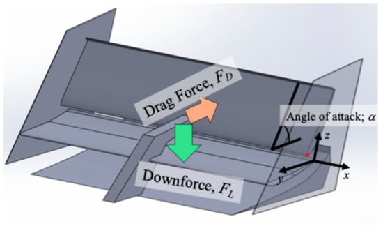
Figure 1. Schematic view of the rear wing.

Since both down force and drag are proportional to the square of speed, air resistance increases rapidly as speed rises. A large negative value for the coefficient of lift (C_L) improves tire–to–ground contact, enhancing grip on the road surface. Conversely, a low coefficient of drag (C_D) reduces air resistance, which in turn improves fuel efficiency.

2.2. Wing Shape and Arrangement

The upper wing must generate a significant amount of downforce even when the DRS is activated, meaning the AOA is shallow. Additionally, it should not be overly thick to minimize weight. Based on these requirements, the E193 shape was adopted, which is also used in the rear wings of actual production vehicles and boasts a high lift–to–drag ratio. In contrast, the lower wing features a thin profile to reduce weight, and its AOA remains relatively constant to maintain low drag, even at slightly steeper angles. Moreover, the DRS mechanism necessitates some warping of the upper portion of the lower wing to function effectively as a wind guide plate for the lower part of the upper wing. Based on these considerations, the BE50 (original) shape was chosen. The cross–sectional shapes of the E193 for the upper wing and the original BE50 for the lower wing are illustrated in Figure 2a,b, respectively. The airfoil geometry is depicted by the red curve, while the blue line illustrates the chord line.

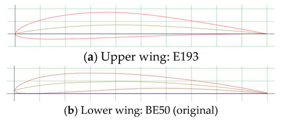
Figure 2. Cross–sectional shape of wings.

The design of the upper wing with DRS activated was carefully considered. Specifically, when DRS is engaged, the two–stage rear wing is positioned almost directly above the lower wing at a shallow AOA, resembling a biplane configuration. This allows the lower wing to function as a wind guide plate for the lower part of the upper wing. Conversely, when DRS is deactivated, the rear wings maintain a multi–stage configuration that remains effective even at steeper angles of attack, similar to conventional designs. This aims to generate maximum downforce from low speeds, regardless of the associated drag.

To facilitate both DRS on and off states with a straightforward mechanism, a sliding variable rear wing mechanism was implemented. The actuator operates in linear motion, akin to traditional DRSs, pushing and pulling the central area in front of the upper wing. A rail is integrated into the wing end plates, with protrusions at both ends of the upper wing that follow this rail to create a sliding mechanism. This allows the upper wing to be positioned optimally in both DRS states. Figure 3 shows a schematic diagram explaining the operation of the DRS. Here, Figure 3a shows the case when DRS is on, and Figure 3b shows the case when DRS is off. Analyses were conducted for both DRS off and on scenarios to fine–tune the wing’s position and establish its relationship in each condition. Additionally, the test vehicle was equipped with a ducktail to serve as a wind guide for the rear wing, which was also subjected to analysis.

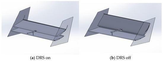
Figure 3. Schematic diagram of the operation of the DRS.

2.3. Target Value

This study focuses on the rear wing for student formula vehicles, with the assumption that the DRS will be utilized on the longest track, approximately 60 m, of a student formula course. The test vehicle weighs approximately 380 kg, including the driver. Figure 4 shows the test vehicle KFR–20. The tires used are Hoosier slick tires (Hoosier Racing Tire, Lakeville, IN, USA), sized 20.5 × 7.0–13, (compound: R25B), as shown in Figure 5. Considering the tire performance data, it is expected that the downforce will exceed 120 N when DRS is off and will be reduced to around 80 N when DRS is engaged while driving at a speed of 60 km/h. The objective is to achieve a significant reduction in drag during this operation.

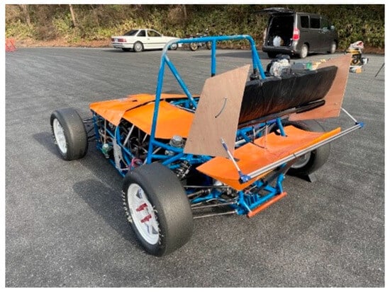
Figure 4. Test vehicle (Student Formula).

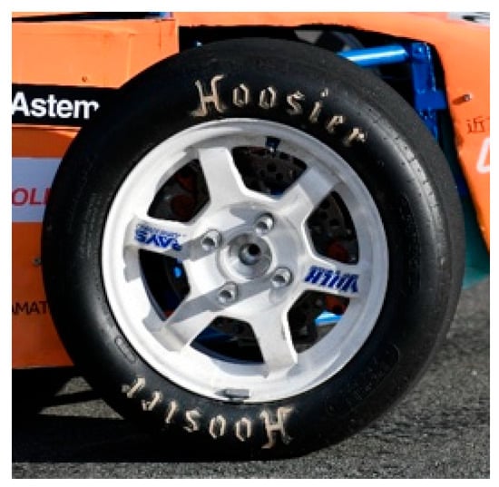
Figure 5. Hosier slick tires.

3. CFD Analysis

3.1. Method

SolidWorks 2022, a 3D CAD software, was used for the design, ensuring that the dimensions conformed to the regulations of the Student Formula. The wing shape was analyzed based on the drag coefficient (C_D) and lift coefficient (C_L) values from Airfoil Tools, specifically using the E193 for the upper section and the BE50 (original) for the lower section, which includes winglets at the trailing edge. For the computational fluid dynamics (CFD) analysis, scFLOW v2022 by Software Cradle was employed. The analysis area was designed to ensure that the size of the computational space did not adversely affect the flow around the analyzed object. In particular, the area behind the wing was enlarged, as the flow in that region can significantly influence the results. Given that the maximum length of the model in this study is 1.1 m in width, this length served as a reference. Consequently, the analysis area extended 2 m in front of and below the wing, 10 m behind the wing, and 5 m above and to the left and right. Figure 6 shows the analysis area and mesh arrangement. The fluid was modeled as incompressible air at 20 degrees centigrade. The vehicle was assumed to be traveling straight ahead at 60 km/h. The boundary condition for inflow was set to 60 km/h, reflecting the assumed vehicle speed, while the outflow boundary condition was defined as static pressure outflow, with a pressure of 0 Pa. As shown in Figure 6, the blue, green, and red regions represent the velocity inlet, the free–slip walls, and the pressure outlet for free inflow/outflow, respectively. For the boundary surfaces in the analysis domain that were not subjected to the inflow–outflow boundary condition, a free–slip condition was applied, whereas the wing surfaces were assigned a no–slip condition. The standard k–ε turbulence model was used, and the analysis was conducted under steady–state conditions, fixed at the DRS configuration.

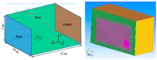
Figure 6. Analysis area and mesh arrangement.

To accurately capture the aerodynamic forces acting on the DRS multi–element wing, a hybrid mesh strategy was employed. The computational domain was discretized using polyhedral meshes, which provide superior convergence and spatial accuracy for complex flow fields compared to standard tetrahedral meshes. The mesh was meticulously refined around the wing elements to resolve the high–pressure gradients and flow separation zones, resulting in a total mesh count of approximately 2.2 million cells. To ensure the reliability of the numerical results, a Grid Convergence Study was conducted using several different mesh densities. Based on the analysis of multiple configurations, it was confirmed that a mesh count of 2.2 million cells provides the optimal balance between spatial resolution and computational time. A mesh sensitivity analysis was performed to verify the reliability of the CFD simulations. Three computational grids with different resolutions were generated by refining the mesh density in the vicinity of the wing surface, with average cell sizes of 0.005 m, 0.002 m, and 0.001 m. The sensitivity of the solution was assessed based on the separation point and integrated aerodynamic forces. The downforce showed negligible variation between the 0.002 m and 0.001 m cases, indicating that the solution had achieved grid independence. Based on these findings, the mesh with an average surface size of 0.002 m (totaling approximately 2.2 million cells) was adopted for all subsequent analyses to minimize discretization errors while maintaining a reasonable computational cost.

Specifically, for the near–wall treatment, a log–law based wall function was applied to the turbulent boundary layer. To ensure the validity of this wall function, the height of the first layer of the inflation mesh was set to 9.5 × 10⁻⁴ m, and five layers of boundary layer mesh were inserted. This specific configuration was determined through preliminary analysis to maintain the average dimensionless wall distance y+ at approximately 50 across the majority of the wing surface at the primary evaluation speeds (20–80 km/h). Since this y+ value is positioned well within the logarithmic region (30 < y+ < 300), the reliability and physical consistency of the wall function are sufficiently guaranteed. The boundary layer mesh was designed with a growth rate of 1.2 across its five layers. This specific gradient ensures a smooth and stable transition from the high–gradient near–wall region to the polyhedral mesh in the far–field, preventing numerical instabilities at the interface. This mesh configuration allows the k–ε turbulence model to appropriately resolve wall shear stress and flow separation characteristics while maintaining the computational efficiency necessary for generating the large–scale datasets required for GNN training. Figure 7 presents the surface pressure distribution and the pressure contour of the wing cross–section as a representative example of the results.

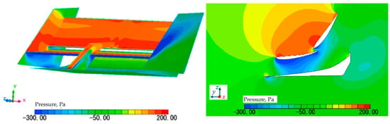
Figure 7. Surface pressure distribution and the pressure contour of the wing cross–section.

3.2. Determining Upper Wing Position and AOA

To determine the optimal DRS configuration, the downforce and drag force were systematically evaluated via CFD by varying the upper wing’s longitudinal position (y), vertical position (z), and Angle of Attack (AOA). The positional definitions are illustrated in Figure 8. The red line indicates the trajectory of the upper wing’s movement in the y–direction, while the orange dots denote the specific wing positions where CFD analyses were conducted. Initial analysis at a fixed configuration (y = 50 mm, z = 40 mm) across a velocity range showed that both aerodynamic forces increase proportionally with fluid velocity (Figure 9). While downforce peaked at an AOA of 40 degrees, the drag force continued to increase up to 50 degrees. This trend is attributed to significant flow separation behind the upper wing at higher angles. Further investigation into the coupling between longitudinal position (y) and AOA (at z = 20 mm) revealed that downforce generally increases with AOA up to 40 degrees. However, at the forward–most position (y = 10 mm), the downforce gains between 40 degrees and 50 degrees become negligible. In contrast, drag force consistently increases as the AOA increases and the longitudinal gap (y) decreases, reflecting the heightened aerodynamic resistance of the multi–element system. Figure 10a illustrates the relationship between the wing’s longitudinal position y, AOA, and the generated downforce, while Figure 10b shows the corresponding relationship with the drag force. As indicated in Figure 10a, the maximum downforce was recorded at 40 degrees. However, the downforce decreases when the AOA is further increased to 50 degrees. This phenomenon is primarily attributed to significant flow separation triggered at the rear of the second wing element when the AOA becomes excessive. As a result, the lift–to–drag ratio deteriorates as the downforce decreases while the drag increases rapidly due to the expanded separation zone.

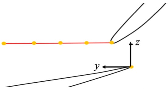
Figure 8. Relative position of the lower wing and upper wing.

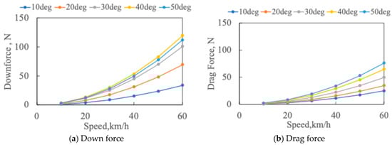
Figure 9. Relation between speed and downforce and drag force at y = 50.

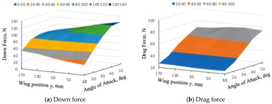
Figure 10. Relationship between wing position, AOA, down force and drag force.

To optimize the DRS, the y, z, and AOA parameters were determined based on aerodynamic performance requirements. For maximum downforce during cornering, an AOA of 40 degrees was selected, with z = 20 mm identified as the optimal vertical separation (Figure 11). Conversely, drag reduction performance was found to improve as the upper wing translates forward (decreasing y, Figure 12) and the AOA decreases (Figure 10). Therefore, the maximum drag reduction is achieved by simultaneously shifting the wing forward and reducing its AOA. In conclusion, high downforce is attained by positioning the upper wing’s leading edge near the lower element’s trailing edge at a high AOA. For high–speed efficiency, the wing should be moved forward with a reduced AOA. This CFD–based methodology successfully establishes a dual–mode operation strategy for both high–downforce cornering and low–drag high–speed performance. Consequently, the optimal DRS strategy involves positioning the wing for maximum downforce during low–speed cornering and translating it forward while reducing the AOA for high–speed operations.

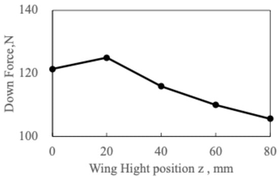
Figure 11. Relationship between wing height position z and down force of AOA a = 40 degrees.

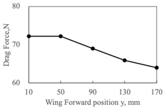
Figure 12. Relationship between wing forward position y and drag force of AOA α = 40 degrees.

3.3. CFD Analysis Results

Table 1 presents the state of downforce, drag force, and lift–to–drag ratio of the rear wing with the mechanism used in this study, comparing conditions with DRS on and off. It is evident that both downforce and drag can be significantly reduced when DRS is activated. Notably, drag decreases substantially, and the lift–to–drag ratio improves from 1.92 to 2.80. The air velocity vector for the DRS off condition is illustrated in Figure 3. Furthermore, the DRS off and DRS on cases are shown in Figure 13a,b, respectively. The results confirm that the upper wing operates efficiently with the lower wing at a shallow angle of attack when DRS is engaged.

Table 1. CFD analysis results.

	Down Force (N)	Drag Force (N)	Lift–to–Drag Ratio
DRS off	138.7	82.68	1.67
DRS on	57.3	25.51	2.67

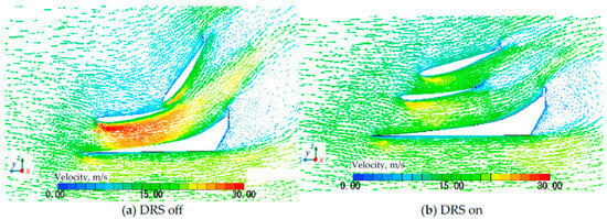
Figure 13. Velocity vectors in cross section.

4. Surrogate Model

4.1. Dataset Design and Acquisition

A surrogate model was constructed using a dataset obtained from executing CFD simulations across a wide range of design parameters. The input space was designed to capture the complex aerodynamic interactions of the DRS by varying four primary parameters:

• Longitudinal position (x): 5 levels;
• Vertical position (z): 5 levels;
• Angle of Attack (AOA; α): 7 levels;
• Velocity (Reynolds number): 6 levels.

This resulted in a total of 1050 discrete geometric and flow combinations. The output data consisted of the corresponding aerodynamic performance coefficients: downforce (F_L), drag force (F_D), and aerodynamic efficiency (C_L/C_D). This high–resolution dataset allows the surrogate model to map the entire performance envelope, which is later utilized for exhaustive optimization.

4.2. Machine Learning Model Selection and GNN Adoption

While candidates such as Gaussian Process Regression (GPR), Support Vector Regression (SVR), and conventional deep learning models exist, handling geometrically coupled systems as complex as DRS necessitates a model capable of directly learning the geometric structure. In this study, the Graph Neural Network (GNN) was adopted as the primary surrogate model. The GNN is employed to effectively model the complex geometric and aerodynamic couplings inherent in the DRS. Unlike traditional fixed–vector input models in the field of aerodynamic design, the GNN directly represents and learns from the wing shape as a graph structure, where vertices denote control points and edges represent adjacency relationships. The detailed architecture of the proposed GNN is illustrated in Figure 14. The network utilizes a message–passing framework designed to propagate physical influences across the aerodynamic graph. The network is designed as a deep message–passing framework consisting of an input layer, multiple hidden graph processing layers, and a regression output layer. The input layer receives a four–dimensional feature vector for each relevant node, corresponding to the vertical (z) and longitudinal (x) relative positions of the second wing element, the angle of attack (AOA; α), and the local geometric curvature. To capture the complex, non–linear interactions within the aerodynamic graph, the hidden architecture utilizes a high–dimensional feature space (400 hidden units per layer). This configuration allows the model to internalize the geometric topology and the resulting pressure field coupling. The output layer consists of two nodes dedicated to the direct prediction of the drag coefficient (C_D) and the lift coefficient (C_L). The core of this model is the message–passing mechanism, which facilitates the transmission of physical influences between elements. The feature vector h_v^(l+1) of node v at layer l + 1 is updated by aggregating messages from its neighborhood N(v) as follows:

$${\mathbf{h}}_v^{\left(l+1\right)}=\sigma \left({\mathbf{W}}^{\left(l\right)}{\mathbf{h}}_v^{\left(l\right)}+\sum _{u\in N\left(v\right)}{\mathbf{M}}^{\left(l\right)}\left({\mathbf{h}}_v^{\left(l\right)},{\mathbf{h}}_u^{\left(l\right)}\right)\right)$$

(3)

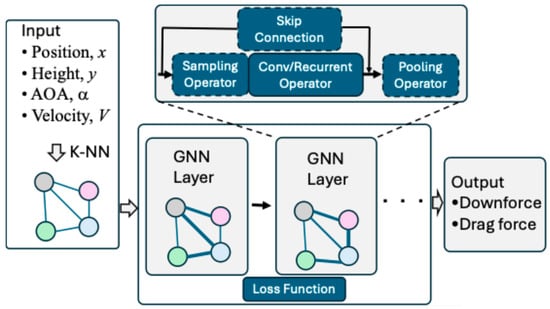
Figure 14. Schematic architecture of the GNN for downforce and drag force prediction.

Here, N(v) represents the set of neighbors of node v, W^(l) is a trainable weight matrix applied to the node’s own information, M^(l)(•) is the message function calculating the information transmitted from the neighbor node u to v, and s is the nonlinear activation function. Through this process, each node on the aerodynamic mesh integrates local neighborhood information, allowing the network to internalize complex coupling phenomena—such as pressure distribution changes caused by flap proximity—consistent with the governing equations of fluid dynamics. Regarding the dataset construction, a total of 1050 CFD simulation cases were initially generated using a Full Factorial Design to cover the entire operational envelope of the wing. From this comprehensive pool, 400 cases were randomly selected as the training dataset for the GNN. This randomized sampling approach from a dense grid ensures that the model is trained on a diverse yet representative distribution of the design space, facilitating better generalization. All input features were normalized to a mean of zero and a standard deviation of one. The optimization and implementation were conducted using the MATLAB 2025a Deep Learning Toolbox.

4.3. Surrogate Model Validation and Convergence

The reliability of the GNN surrogate model was validated through a twofold approach: monitoring training convergence and comparing predictions against unseen CFD benchmarks. First, to evaluate the stability and efficiency of the learning process, the loss curves for both training and validation phases were analyzed, as shown in Figure 15. The Mean Squared Error (MSE) exhibits a sharp initial decline followed by a stable convergence to a minimal error floor. The fact that the validation loss consistently tracks the training loss without significant divergence demonstrates that the 400–node pattern layer successfully internalized the flow physics and spatial features without overfitting the training data. This convergence behavior confirms that the exhaustive grid search provided a sufficiently dense manifold for the GNN to learn the underlying aerodynamic correlations. Second, the quantitative accuracy was evaluated by comparing GNN predictions with CFD results for test cases within the exhaustive grid that were excluded from the initial training phase. As shown in Figure 16, the model demonstrates exceptional fidelity. The blue dots show the data points from both the CFD and surrogate model, and the red line signifies the identical value threshold between them. For downforce, the MSE was 7.39, corresponding to a prediction error of 2.7 N or less. For drag, the error was 1.29 N or less. The coefficient of determination (R²) exceeded 0.99 for both parameters, indicating that the GNN faithfully reproduces the complex aerodynamic couplings of the DRS across the entire exhaustive design space.

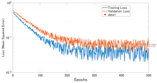
Figure 15. Loss curves for training and validation and best model (minimum validation loss).

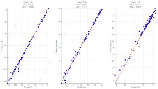
Figure 16. Comparison of GNN estimates and CFD results.

5. Experiments Using Student Formula Vehicle

5.1. Laboratory Validation Methodology for the Wing Unit

To validate the GNN model’s predictions, physical experiments were conducted in a controlled laboratory environment using a full–scale rear wing prototype. The prototype was modeled using 3D–CAD software and featured an aluminum pipe internal framework shaped with Styrofoam, finished with smooth wrapping sheets. Plywood was utilized for the wing end plates to ensure structural rigidity.

The experimental setup is illustrated in Figure 17. An electric fan was positioned 1 m away from the leading edge of the main wing element to provide a constant airflow of 10 m/s. In the experimental setup, the distance between the electric fan and the rear wing was carefully calibrated to ensure a consistent inflow condition. Specifically, the separation distance was adjusted such that the mean airflow velocity, measured at the plane of the wing’s leading edge, was maintained at a constant 10 m/s. This calibration accounted for the velocity fluctuations inherent near the fan exit, ensuring a stable area–averaged velocity for the duration of the tests. Aerodynamic vertical loads were measured using strain gauges mounted on four support pillars connecting the wing unit to the base. The pillars consisted of A6063 aluminum alloy tubes with a diameter of 10 mm and a wall thickness of 1.0 mm, characterized by a Young’s modulus of 68.3 GPa. Data acquisition was performed using a TML DC–204R dynamic strain meter. Strain levels were measured at four distinct locations using a quarter–bridge (1–gauge) method at a sampling frequency of 100 Hz. The recorded strain values were converted into vertical loads based on the pillar’s material properties and summed to calculate the total downforce. A moving average filter was applied to the raw data to mitigate experimental noise, establishing a rigorous methodology for comparing the measured aerodynamic forces with the coefficients predicted by the GNN model.

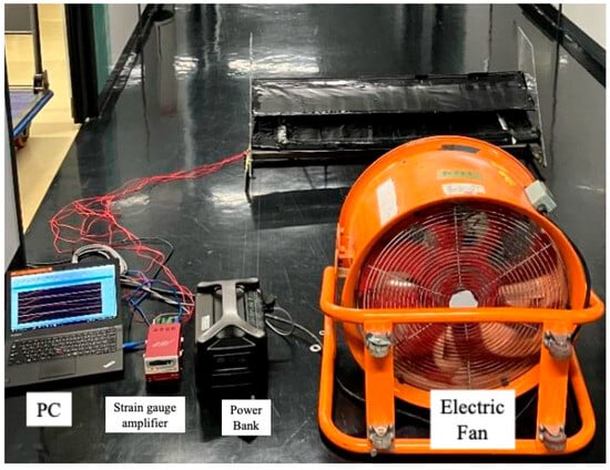
Figure 17. Laboratory experimental setup for aerodynamic force measurement.

Following the laboratory unit validation, the optimized sliding DRS mechanism was implemented on a Formula SAE vehicle to verify its operational functionality. The sliding DRS was realized by actuating the framework at the leading edge of the upper wing, allowing its rear end to move along dedicated rails integrated into the wing end plates (Figure 18).

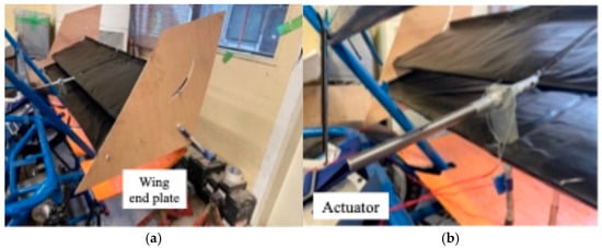
Figure 18. Wing end plate and DRS actuator.

The integration strategy focused on the synergy between mechanical performance and electronic control. The mechanical actuators were interfaced with the vehicle’s electronic control unit (ECU) to enable rapid and reliable transitions between high–downforce and low–drag configurations during dynamic operation. Functional testing on the actual vehicle was conducted to verify that the mechanism maintained its structural integrity and operational reliability under aerodynamic loads during vehicle maneuvers. This multi–stage approach—from laboratory validation of the standalone unit to integration with the vehicle’s control systems—ensures that the GNN–driven design meets the practical requirements of a competitive racing environment.

5.2. Measured Experimental Results

The rear wing, including the sliding DRS mechanism, was subjected to experimental testing to validate the CFD analysis and evaluate its real–world performance. Key metrics such as downforce, drag, and the lift–to–drag ratio were measured at various speeds, both with DRS on and off. The results were compared to the predictions from the simulations, and any discrepancies were analyzed to understand the behavior of the wing under actual driving conditions.

The maximum relative error between the analysis results and the actual measured values was 8.14%, indicating a satisfactory level of analysis accuracy. Factors contributing to this error include the instability of the fan–generated wind, the manufacturing precision of the rear wing, and the slight up–and–down oscillation of the rear wing, which affected the reaction values. Table 2 presents a comparison between the experimental data measured by strain gauges and the CFD analysis results for both “DRS off” and “DRS on” conditions. The measured aerodynamic force decreased from 14.35 N to 10.64 N when the DRS was activated. The relative errors between the experimental and numerical results were 8.14% and 6.40%, respectively, showing a good correlation between the two methods.

Table 2. Experimental results using strain gauges.

	DRS Off	DRS ON
Experimental Results	14.35 N	10.64 N
CFD Analysis Results	13.37 N	10.0 N
Relative Error	8.14%	6.40%

The operational states of the Drag Reduction System (DRS) in this study are categorized into “DRS Off” and “DRS On” modes. As illustrated in Figure 13a, the DRS Off configuration maintains the wing in a fully closed state across the entire velocity range to prioritize maximum downforce. In contrast, the DRS On configuration dynamically adjusts the upper wing element according to the vehicle’s speed. Specifically, the wing begins to translate and change its angle of attack (AOA) once the velocity exceeds 33.3 km/h. As the speed increases, the flap moves progressively toward the open position, reaching the fully open state shown in Figure 13b at a velocity of 66.6 km/h.

The performance of the rear wing with DRS was further evaluated on a student formula car. Tests were conducted by entering the starting point at 20 km/h, with DRS both on and off, and measuring the maximum speed and acceleration time over a 50 m straight–line sprint. The experimental results are summarized in Table 3. These findings confirm that the primary objectives of the DRS—improving acceleration in straight sections and increasing maximum speed—were successfully achieved using the sliding mechanism developed in this study.

Table 3. Experimental results using student formula car.

	DRS Off	DRS ON	Improvement
50 m acceleration time	5.735 s	5.470 s	4.6%
Maximum speed	77.0 km/h	81.5 km/h	5.8%

6. Conclusions

This research successfully demonstrated a high–fidelity optimization framework for a sliding Drag Reduction System (DRS) by using Graph Neural Network (GNN) surrogate models. To overcome the high computational costs of conventional CFD, a GNN-based approach was implemented to directly learn from the geometric graph structure of the multi-element wing. This allowed for the accurate modeling of complex aerodynamic couplings between the sliding upper wing, the main element, and the ducktail guide, facilitating an efficient exploration of the design space.

The optimization achieved through the GNN model results in significant drag reduction primarily through two mechanisms. First, the reduction in the projected area S leads to a direct decrease in pressure drag (form drag). Second, the optimized relative positioning of the second flap element influences the circulation of the main element. By optimizing the gap and overlap, the high–velocity flow passing through the slot delays flow separation on the flap’s suction side. Furthermore, the GNN identified a configuration that suppresses the strength of trailing–edge vortices, effectively reducing induced drag during high–speed operation.

The key outcomes of this study are as follows:

• GNN Surrogate Model Efficacy: The GNN model effectively captured the complex geometric relationships of the DRS, achieving an R² value exceeding 0.99 for both lift and drag coefficients. With a Mean Squared Error for downforce of 7.39, the model proved to be a robust, low–latency alternative to traditional CFD for iterative design optimization.
• Aerodynamic Performance Optimization: Through the GNN–facilitated optimization, a sliding mechanism was finalized that reduces drag from 82.68 N to 25.51 N upon activation. This resulted in a significant improvement in the lift–to–drag ratio from 1.67 to 2.67, confirming the efficiency of the biplane–like configuration in the “DRS on” state.
• Experimental Validation of the AI Framework: Physical measurements via strain gauges corroborated the GNN–predicted trends with a maximum relative error of 8.14%. This high degree of correlation validates the reliability of using graph–based neural networks for predicting real–world aerodynamic forces in racing applications.
• Operational Success: Field testing of the KFR–20 Student Formula vehicle confirmed the practical utility of the optimized design. The implementation of the DRS resulted in a 4.6% reduction in 50 m acceleration time and a 5.8% increase in maximum speed (from 77.0 km/h to 81.5 km/h).

The study concludes that GNNs are capable of approximating CFD results with high precision while significantly reducing the time required for aerodynamic optimization. By capturing the intricate physical influences within the DRS assembly, this framework enables a more comprehensive design exploration than traditional methods. Ultimately, the integration of GNN-based surrogates offers a robust and scalable solution for the rapid development of high-performance aerodynamic components in automotive engineering.

Although the current GNN architecture demonstrates significant potential in capturing geometric dependencies, further investigation is required to quantitatively assess its relative superiority over conventional methods. As a primary direction for future research, we intend to conduct a comprehensive comparative analysis of the proposed GNN model against traditional surrogate modeling techniques, such as Multi–Layer Perceptrons (MLP) and Polynomial Regression (PR). This investigation will focus on identifying the trade–offs between predictive precision and computational costs, specifically regarding training duration and inference latency.

This research successfully demonstrated a high-fidelity optimization framework for a sliding Drag Reduction System (DRS) by employing Graph Neural Network (GNN) surrogate models. The primary bottleneck in aerodynamic development—the high computational cost of CFD and the complexity of physical testing—was addressed by utilizing a GNN that directly learns from the geometric graph structure of the multi-element wing. This approach allowed for the faithful modeling of physical influences and aerodynamic couplings between the sliding upper wing, the main element, and the ducktail guide. The study concludes that GNNs are not only capable of approximating CFD results with high precision but also enable a more comprehensive exploration of the design space, leading to an optimized DRS configuration that significantly enhances vehicle performance.

References

- Coiro, D.; Nicolosi, F.; Amendola, A.; Barbagallo, D. Experiments and Numerical Investigation on a Multi–Component Airfoil Employed in a Racing Car Wing; SAE Technical Paper 970411; SAE International: Warrendale, PA, USA, 1997. [Google Scholar] [CrossRef]
- Garry, K.P. Some effects of ground clearance and ground plane boundary layer thickness on the mean base pressure of a bluff vehicle type body. J. Wind. Eng. Ind. Aerodyn. 1996, 62, 1–10. [Google Scholar] [CrossRef]
- Jasinski, W.; Selig, M. Experimental Study of Open–Wheel Race–Car Front Wings; SAE Technical Paper 983042; SAE International: Warrendale, PA, USA, 1998. [Google Scholar] [CrossRef]
- Guerrero, A.; Castilla, R.; Eid, G. A Numerical Aerodynamic Analysis on the Effect of Rear Underbody Diffusers on Road Cars. Appl. Sci. 2022, 12, 3763. [Google Scholar] [CrossRef]
- Zhang, X.; Toet, W.; Zerihan, J. Ground Effect Aerodynamics of Race Cars. Appl. Mech. Rev. 2006, 59, 33–49. [Google Scholar] [CrossRef]
- Yudianto, A.; Susanto, H.A.; Suyanto, A.; Adiyasa, I.W.; Yudantoko, A.; Fauzi, N.A. Aerodynamic performance analysis of open–wheel vehicle: Investigation of wings installation under different speeds. J. Phys. Conf. Ser. 2020, 1700, 012086. [Google Scholar] [CrossRef]
- Katz, J. Aerodynamic Model for Wing–Generated Down Force on Open–Wheel–Racing–Car Configurations; SAE Paper 860218; SAE International: Warrendale, PA, USA, 1986. [Google Scholar] [CrossRef]
- Ahangarnejad, A.H.; Melzi, S.; Ahmadian, M. Integrated Vehicle Dynamics System through Coordinating Active Aerodynamics Control, Active Rear Steering, Torque Vectoring and Hydraulically Interconnected Suspension. Int. J. Automot. Technol. 2019, 20, 903–915. [Google Scholar] [CrossRef]
- Mears, A.P.; Dominy, R.G.; Sims–Williams, D.B. The Air Flow About an Exposed Racing Wheel; SAE Technical Paper 2002–01–3290; SAE International: Warrendale, PA, USA, 2002. [Google Scholar] [CrossRef]
- Ranzenbach, R.; Barlow, J. Cambered Airfoil in Ground Effect—An Experimental and Computational Study; SAE Technical Paper 960909; SAE International: Warrendale, PA, USA, 1996. [Google Scholar] [CrossRef]
- Loução, R.; Duarte, G.; Mendes, M.J. Aerodynamic Study of a Drag Reduction System and Its Actuation System for a Formula Student Competition Car. Fluids 2022, 7, 298. [Google Scholar] [CrossRef]
- Kajiwara, S. Passive variable rear–wing aerodynamics of an open–wheel racing car. Automot. Engine Technol. 2017, 2, 107–117. [Google Scholar] [CrossRef]
- Nath, S.D.; Pujari, P.C.; Jain, A.; Rastogi, V. Drag reduction by application of aerodynamic devices in a race car. Adv. Aerodyn. 2021, 3, 4. [Google Scholar] [CrossRef]
- Bleeker, M.; Dorfer, M.; Kronlachner, T.; Sonnleitner, R.; Alkin, B.; Brandstetter, J. Neuralcfd: Deep learning on high–fidelity automotive aerodynamics simulations. arXiv 2025, arXiv:2502.09692. [Google Scholar]
- Dube, P.; Hiravennavar, S. Machine Learning Approach to Predict Aerodynamic Performance of Underhood and Underbody Drag Enablers; SAE Technical Paper 2020–01–0684; SAE International: Warrendale, PA, USA, 2020. [Google Scholar] [CrossRef]
- Bekemeyer, P.; Hariharan, N.; Wissink, A.M.; Cornelius, J. Introduction of Applied Aerodynamics Surrogate Modeling Benchmark Cases. In Proceedings of the AIAA SCITECH 2025 Forum, Orlando, FL, USA, 6–10 January 2025. [Google Scholar]
- Guo, X.; Li, W.; Iorio, F. Convolutional Neural Networks for Steady Flow Approximation. In Proceedings of the 22nd ACM SIGKDD International Conference on Knowledge Discovery and Data Mining (KDD’16), San Francisco, CA, USA, 13–17 August 2016; pp. 481–490. [Google Scholar] [CrossRef]
- Thuerey, N.; Weissenow, K.; Prantl, L.; Hu, X.Y. Deep Learning Methods for Reynolds–Averaged Navier–Stokes Simulations of Airfoil Flows. AIAA J. 2018, 58, 25–36. [Google Scholar] [CrossRef]
- Sekar, V.; Zhang, M.; Shu, C.; Khoo, B.C. Inverse Design of Airfoil Using a Deep Convolutional Neural Network. AIAA J. 2019, 57, 993–1003. [Google Scholar] [CrossRef]
- Kashefi, A.; Rempe, D.; Guibas, L.J. A Point–Cloud Deep Learning Framework for Prediction of Fluid Flow Fields on Irregular Geometries. arXiv 2020, arXiv:2010.09469. [Google Scholar] [CrossRef]
- Raissi, M.; Perdikaris, P.; Karniadakis, G.E. Physics–Informed Neural Networks: A Deep Learning Framework for Solving Forward and Inverse Problems Involving Nonlinear Partial Differential Equations. J. Comput. Phys. 2019, 378, 686–707. [Google Scholar] [CrossRef]
- Zhang, C.; Hu, Z.; Shi, Y.; Xu, G. Fast Aerodynamic Prediction of Airfoil with Trailing Edge Flap Based on Multi–Task Deep Learning. Aerospace 2024, 11, 377. [Google Scholar] [CrossRef]
- Bouhlel, M.A.; He, S.; Martins, J.R.R.A. Scalable Gradient–Enhanced Artificial Neural Networks for Airfoil Shape Design in the Subsonic and Transonic Regimes. Struct. Multidiscip. Optim. 2020, 61, 1363–1376. [Google Scholar] [CrossRef]
- Chen, W.; Chiu, K.; Fuge, M.D. Airfoil Design Parameterization and Optimization Using Bézier Generative Adversarial Networks. AIAA J. 2020, 58, 4723–4735. [Google Scholar] [CrossRef]
- Jacob, S.J.; Mrosek, M.; Othmer, C.; Köstler, H. Benchmarking Convolutional Neural Network and Graph Neural Network Based Surrogate Models on a Real–World Car External Aerodynamics Dataset. Comput. Fluids 2025, 300, 106760. [Google Scholar] [CrossRef]
- Pozdnyakov, S.N.; Ceriotti, M. Incompleteness of Graph Neural Networks for Point Clouds in Three Dimensions. arXiv 2022. [Google Scholar] [CrossRef]
- Sun, L.; Gao, H.; Pan, S.; Wang, J.–X. Surrogate Modeling for Fluid Flows Based on Physics Constrained Deep Learning Without Simulation Data. Comput. Methods Appl. Mech. Eng. 2020, 361, 112732. [Google Scholar] [CrossRef]
- Kashinath, K.; Mustafa, M.; Albert, A.; Wu, J.L.; Jiang, C.; Esmaeilzadeh, S.; Azizzadenesheli, K.; Wang, R.; Chattopadhyay, A.; Singh, A.; et al. Physics Informed Machine Learning: Case Studies for Weather and Climate Modelling. Philos. Trans. R. Soc. A Math. Phys. Eng. Sci. 2021, 379, 20200093. [Google Scholar] [CrossRef]
- Zhu, L.; Zhang, W.; Kou, J.; Liu, Y. Machine Learning Methods for Turbulence Modeling in Subsonic Flows Around Airfoils. Phys. Fluids 2019, 31, 015105. [Google Scholar] [CrossRef]
- Catalani, G.; Agarwal, S.; Bertrand, X.; Tost, F.; Bauerheim, M.; Morlier, J. Neural Fields for Rapid Aircraft Aerodynamics Simulations. Sci. Rep. 2024, 14, 25496. [Google Scholar] [CrossRef] [PubMed]
Disclaimer/Publisher’s Note: The statements, opinions and data contained in all publications are solely those of the individual author(s) and contributor(s) and not of MDPI and/or the editor(s). MDPI and/or the editor(s) disclaim responsibility for any injury to people or property resulting from any ideas, methods, instructions or products referred to in the content. |
© 2026 by the authors. Licensee MDPI, Basel, Switzerland. This article is an open access article distributed under the terms and conditions of the Creative Commons Attribution (CC BY) license.