Abstract
Turbulence is a complex and challenging concept, often simplified for students through the use of the Reynolds Number (Re), used to indicate when flow transitions from laminar to turbulent occurs. However, the Re number focus on the ratio of inertial to viscous forces limits its ability to explain the physical mechanisms driving turbulence, particularly in cases involving different flow boundaries or two-phase stratified flows including flows with phase change. This article presents the development and reasoning of the Shear number (Sn) as a new turbulence indicator, based on the ratio of shear to viscous forces, which provides a more intuitive and accurate representation of turbulence initiation. By comparing Sn to Re, this study demonstrates how the Sn number enhances the understanding of turbulent flow and offers a more accessible tool for both teaching and practical applications in fluid dynamics.
1. Introduction
Many teachers tell students that turbulence is a very complex topic. Even the famous physicist R. Feynman [1] said it is “the most important unsolved problem of classical physics”. This might make some students feel that understanding turbulence is impossible, so they just memorize some numbers for tests: turbulence occurs when the Reynolds number (Re) is over 4000 and does not occur if it is below 2000. However, the definition of the Reynolds number as the “ratio of inertial forces to viscous forces” is not very helpful. It is easier to think about ratios that are just above or below one, as these can be interpreted as “stronger” or “weaker”. However, a ratio where one force is 4000 times bigger than the other is hard to imagine, making it tough to understand why a fluid flow would change so much when this ratio goes below 2000. The well-known Reynolds number (Re) remains one of the most important concepts in both practice and history of science, but it has some limitations, such as surface roughness evaluation, two-phase separated flow application, and especially when it comes to teaching its physical meaning to students. Summarized Reynolds numbers in parallel shear flows are provided in the review by [2]. Key points include energy stability at Re = 81.5; appearance of critical state near Re = 773; experimental indication of turbulence near Re ≈ 1600; critical Re ≈ 2040 from splitting and decay balance; weak slug spreading above Re ≈ 2250; strong spreading near Re = 2900. However, the review notes that for developing flows, local Reynolds variations must be considered.
Other significant studies of turbulence in fluid flow within a pipe will be discussed next. Wygnanski et al. [3,4] identified two distinct turbulent states, termed “puffs” and “slugs”. A puff was described as a turbulent region with a sharp upstream boundary and a blurred downstream edge that gradually dissipates. These were observed for 2000 < Re < 2700, typically spanning 20–30 pipe diameters in length. Puffs propagate downstream, either decaying back to laminar flow or splitting to form new puffs. In contrast, slugs were characterized by well-defined upstream and downstream boundaries enclosing turbulence across the entire pipe cross-section. Slugs appeared at Re > 3200 and did not relaminarize. Wygnanski et al. considered only the slugs to be associated with the transition from laminar to turbulent flow. The investigation of “puffs” and “slugs” structures in transitional flows using direct numerical simulation (DNS) has been conducted by many researchers [5,6,7,8,9,10]. Their studies demonstrate that numerical solutions of the Navier–Stokes equations now qualitatively replicate experimental observations of these turbulent structures. Darbyshire and Mullin [11] employed impulsive perturbations to determine the stability curve for finite-amplitude disturbances, defining amplitude as the perturbation mass injection rate to total mass flux ratio. Transitions occurred when disturbances surpassed this threshold amplitude, while disturbances with subcritical amplitude decayed downstream. Later investigations by Draad et al. [12] demonstrated that the threshold amplitude exhibits a strong dependence on perturbation frequency. However, research focus shifted from turbulence initiation mechanisms to understanding its self-sustenance. Jimenez and Moin [13] introduced the concept of a minimal channel flow unit—reducing spanwise and streamwise dimensions to the smallest scale capable of maintaining turbulence in DNS. Notably, Waleffe [14,15,16] developed a numerical continuation method transforming fragmented analyses into a unified framework, producing precise nonlinear steady state and traveling wave solutions in plane Poiseuille and Couette flows. These states combine three flow structures—streamwise vortices (rolls), streaks, and instability waves (streak instabilities)—that mutually sustain each other against viscous dissipation. Termed exact coherent structures (ECS), these solutions act as organizing centers for turbulence quasi-cycles by encapsulating the self-reinforcing cycle of streak instability triggering vortices that regenerate streaks. This symbiotic interaction mirrors the self-sustaining process observed in minimal flow units, where turbulence persists through nonlinear feedback between streak breakdown and vortex formation.
With new advanced techniques, the initiation and intensity of turbulence in the “transition region” are attracting more research attention. We presented these attempts extensively in reference [17]. For some types of flows, it is not an adequate indicator for the laminar-to-turbulent flow transition, this is documented in our recent studies of stratified vapor-liquid flow regimes [17,18]. The studies show that for flows during which phase change occurs, the transition from laminar to turbulent can occur at significantly different values of the Re number. The underlying physical mechanism responsible for this phenomenon can be attributed to the fact that the initiator of turbulence is not the inertial force of the fluid itself, but rather the shear force generated by transverse velocity gradients. If the boundaries of the flow are different, these gradients are also different at each individual wall or interface. Among others, C. Liu [19] also proposed a different theory on turbulence generation, which negates the classical concept of vortex breakdown. According to their direct numerical simulation (DNS) observations, all small length scales (it is y+=1–10 in their simulation) are generated by “shear layer instability” rather than vortex breakdown. This shear layer instability is produced by a large vortex structure with multiple level vortex rings, sweeps, ejections, and positive and negative spikes near the laminar sub-layers.
Since the classic Reynolds number does not apply well to all flow cases, it was modified to suit specific needs. When describing wall-bounded turbulence—i.e., the flow of a viscous fluid in a boundary layer close to a wall—the frictional Reynolds number is the preferred choice [20]. It uses friction velocity, and the characteristic dimension is typically taken as the thickness of the boundary layer or half the channel height. The friction velocity, also known as shear velocity, is defined as u* = (τ/ρ)½, where τ represents the shear stress at the boundary. Its application became widespread in turbulent flows with significant wall influence, especially in DNS calculations [21,22]. The critical values of the frictional Reynolds number differs from the classical one. According to Tsukahara et al. [22], Wu and Moin [23], and Duggleby et al. [24], the transitional flow regime begins when Reτ = 60–80, and the turbulent regime begins at approximately Reτ = 180 [21].
In single-phase flow within a circular channel, the boundary around the flowing fluid is uniform. The definitions of the classic Re number are presented in Equations (1) and (3):
The Re number is expressed using standard approximations and notation. Here, m, a, A, and V represent the mass, acceleration, unit area of cross-section, and volume of the fluid element, respectively. L is the characteristic linear dimension, u is the velocity component in the x direction, and A represents the unit area of the cross-section in the numerator and the lateral surface in the denominator. For steady flow, which is mainly in the x direction, du/dt can be written as follows:
where du/dx is velocity change with position, and dx/dt is flow velocity u [25]. Fluid element volume, V, is proportional to characteristic linear dimension L and unit area of cross-section A, the velocity u in the flow field is proportional to bulk velocity U, and du/dx and du/dy are proportional to U/L. Then,
For flows where the fluid boundaries are not the same, the velocity gradients will be different, leading to different shear forces, initiating the turbulence. A suitable indicator for the transition from laminar to turbulent flow should account for these variations. This consideration resulted in the introduction of the “Shear number” (Sn):
In this context, corresponds to shear force at the boundary j, while denotes the related viscous forces. The flow from different sides may be restricted by different surfaces, i.e., the roughness of the different walls may be different, or one of them may be a gas–liquid interface (in the case of an open channel or stratified two-phase flow). For example, Equation (4) outlines the Sn number with an extension for two-phase stratified channel flows, which is discussed in more detail in our work [17].
The concept of the Sn number is not without precedent in the scientific literature. Indeed, related endeavors have been undertaken with the Boundary layer number [26], which serves as a useful point of comparison:
where τw is the shear at the wall, U∞ is the flow velocity far from the boundary layer, and δ is the thickness of the boundary layer. The Boundary layer number, N, is presented in the dimensionless physical quantities handbook [26], but its application has not been widely adopted. The application of this criterion focuses on the flow in the boundary layer, so the characteristic dimension is the thickness of the boundary layer.
The analysis of flows in channels with different boundary characteristics is a more advanced topic, typically addressed in advanced courses. The Sn number is suggested as a teaching tool in introductory courses because it directly relates to the cause of turbulence, making it simpler to explain and comprehend.
2. Development of Shear Number
While the Sn number has a multitude of potential applications, this chapter will limit its scope to the most straightforward case. In the single-phase flows within channels that have uniform boundaries, the shear force at the wall is determined by the bulk velocity and the relevant friction factor, f (Ref. [27] for laminar flow and Ref. [28] for turbulent). This leads to the formulation of the Sn number as follows:
Substituting “shear force” for “inertial force” in a turbulence indicator means using a “direct cause” instead of something that is proportional to turbulence. Table 1 provides an example at room temperature, showing that a moderate improvement can still be achieved even when using an approximate version of Sn’, where the viscous force term is the same as the one used for the Re number.

Table 1.
Approximate Sn’ number for water flow in a pipe, evaluated at T = 25 °C and D = 0.02 m.
The initial two velocities in Table 1 correspond to laminar flow, while the third velocity results in turbulent flow. Ideally, if the nature of the flow remains unchanged, the flow regime indicator should also remain unchanged. A change should indicate that a transition in the flow regime has occurred. As demonstrated, the approximate Sn’ version meets this requirement by staying steady for laminar flows and rising when the flow turns turbulent.
Re and Sn’ both express a ratio of forces, but a critical ratio of 8 is easier to understand and interpret compared to a ratio of 2000, making the Sn’ number more preferable in this regard. However, there is potential for improvement. The students are taught that “laminar” flow suggests order, meaning forces are balanced. The ratio of the shear force that initiates turbulence to the viscous force that dampens it should be 1. So why is it equal to 8 then?
The shear force is determined using the experimentally validated friction factors of Fanning. Therefore, the reason why the Sn’ ratio deviates from 1 is due to the viscous force at the boundary wall being underestimated. This is expected, as the accurate formula for the viscous force is as follows:
where U(r) denotes velocity as a function of the radius. However, in the case of Sn’, the velocity gradient at the boundary is estimated as (U/D). The practice of using D to calculate an approximate linear velocity gradient originates from the 19th century, but utilizing the radius R would yield a more precise estimate for laminar flow, reducing the Sn’ number to 4.
While this is an improvement, the term of viscous force remains underestimated. Fortunately, the equilibrium velocity profile for laminar flow within a pipe is known and can be described as a function of the radius, r:
The derivative of U(r) is then expressed as follows:
At the pipe boundary, Umax is approximately 2Uav, with r equal to R. The terms Umax and Uav denote the maximum and average velocities, respectively. By substituting these values, we find that for laminar flow in a pipe, the gradient at the wall is as follows:
By substituting (10) into (7) and then (7) into (5), the final form of the Sn number can be derived as follows:
At this stage, the Sn number for laminar flow is reduced to 1. To demonstrate this, we utilize the Fanning friction factor, which is defined as 16/Re for laminar flow. Substituting this expression into Equation (11) yields the following:
The claim that the Sn number represents “the ratio of shear to viscous forces” now carries a verifiable physical interpretation—for laminar flow, these forces must be perfectly balanced, meaning the Sn number should be equal to 1.
3. Sn Number Application for Pipe Flow
The generalized Sn expression can be written as follows:
We calculate the components of Sn at various boundaries and sum them by applying the proportionality coefficient, which is based on the ratio of the partial perimeter where shear forces act. The flow cross-section perimeter is P = Pin + Pwj, Pin is the interface perimeter, and Pwj is the wetted wall perimeter at different walls with different roughness.
For fluid flow in a circular pipe with uniform walls (see Figure 1a), the Sn expression in Equation (13) simplifies significantly:
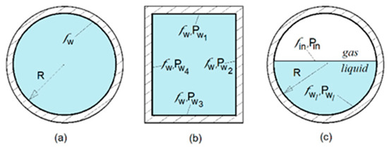
Figure 1.
Flow cross-section: (a) circular pipe; (b) rectangular pipe; (c) circular pipe, gas–liquid flow.
Here are three examples of Sn applications for single-phase and two-phase flow in both circular and rectangular pipes (see Figure 1).
For fluid flow in a rectangular pipe with walls of different roughness (see Figure 1b), the shear at each wall must be evaluated separately, and the Sn components should be summed based on the ratio of partial perimeter:
Here, Req represents the equivalent radius of the rectangular pipe cross-section, while fw1 denotes the friction factor associated with a particular wall.
A more complicated scenario involves separated liquid–gas flow (Figure 1c), which incorporates an interfacial shear estimation component on the liquid side. This additional component estimates friction at the interface fin and gas velocity Ul influence:
Here, the total perimeter of the liquid side is expressed as Pl = Pin + Pw,l, where Pin denotes the perimeter of the interface and Pw,l represents the perimeter of the wetted wall within the liquid. This equation can also be applied to the gas side.
4. Sn Number for Smooth and Rough Pipe Flow
In laminar flow, shear force and viscous force are balanced. The turbulent transition begins when the shear force at the boundary surpasses the viscous force, which is directly proportional to the molecular viscosity and relevant velocity gradient. When this happens, the molecule-to-molecule energy transfer rate is not able to dissipate the energy generated by the shear force, as a result, local eddies are formed. The effective dissipation rate then increases; however, the denominator of the Sn number is evaluated using the molecular viscosity, causing the Sn number to exceed 1. For instance, at liquid velocities of 0.04 and 0.08 m/s, the Sn number is 1, but it increases to 2.3 as the bulk velocity reaches 0.16 m/s.
Figure 2 illustrates the relationship between turbulence indexes and fluid velocity. The figure demonstrates that Sn number provides additional information about flow regime character and transition. While the dependence of the Re number on velocity remains constant during the transition from laminar to turbulent flow, the Sn number clearly reflects the differences between these regimes. Furthermore, as illustrated in Figure 2, the Re number remains unaffected by surface roughness, whereas this influence is evident in the Sn number trend and magnitude. Examples of surface roughness for “smooth” and “very rough” pipes are also provided.
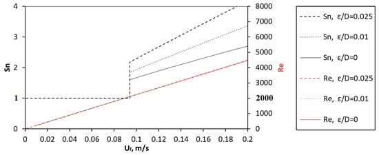
Figure 2.
Sn vs. Re number depending on water bulk velocity in a pipe with a surface roughness of 0, 0.2, 0.5 mm (D = 0.02 m).
The differences between the Re and Sn numbers presented are sufficient to recommend the Sn number for students in introductory courses. The Sn number offers different physical character for laminar and turbulent flow regimes, helps to understand better the physical reasons for the transition to turbulence, and does not require memorizing some critical values.
5. Sn and Turbulence Issues
For more advanced courses that venture deeper into turbulence issues, the Sn number has some additional advantages. For example, it can provide a connecting link between two of the most important historical insights into the nature of turbulence. This is illustrated in the figures that follow, Figure 3 shows a schematic of the “turbulence energy cascade” [29] (based on Richardson (1922)), which is used to explain the Kolmogorov theory (1941) [30], so the actual historical sequence is reversed.
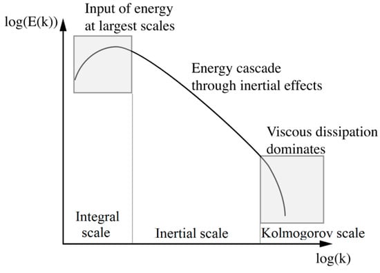
Figure 3.
Schematic representation of energy cascade.
Where E(k) is the turbulent energy of eddies, k is the eddy wave number, which is inversely proportional to eddy size. Kolmogorov recognized that turbulence is a dynamic process in which the kinetic energy of macro-size eddies in the first stage is distributed by inertial interactions to ever smaller eddies and is finally dissipated as thermal energy by molecular viscosity. Indeed, the experimental and DNS findings [31] show that the spectral structure of small-scale fluctuations is governed by the Kolmogorov small-scale hypothesis. It confirms that this phenomenological theory of turbulence may truly be universal.
For flow in a pipe, shear at the wall converts a fraction of the axially directed kinetic energy of the fluid into the three-dimensional turbulent energy of macro-size eddies, by inertial interactions, these eddies split up and their energy is redistributed to ever smaller eddies. The “inertial” subregion can extend over many orders of magnitude. When the eddy size approaches the size of inter-molecular distances their kinetic energy becomes part of the thermal energy of the fluid.
From this simplified description it can be inferred that the Sn number represents the ratio of the rate of turbulent energy generation in the first subregion and its dissipation rate in the final, third subregion. The “inertial” subregion, though not included in the definition of Sn, does influence it by introducing a time element. Redistribution of turbulent kinetic energy from the macro scale eddies to ever smaller eddies requires a very large number of inertial interactions. This takes time, for a flowing fluid this time can be interpreted in terms of distance in the flow direction. With this in mind, consider the drawing in the original 1883 publication by O. Reynolds [32], which defined the relationship between the transition to turbulence and the property ratio that later became known as the Re number.
The historical Figure 4 is a reminder that Reynolds introduced the marking dye, which allowed visualization of turbulence in the center of the test pipe. Reynolds recognized that the transition to turbulent flow depends also on such factors as entrance effects and wall roughness, to account for the resulting uncertainty, he specified a Re number “transition range” from 2000 to 4000. The empirical database has expanded considerably; however, the bracketing Re number values specifying that somewhere within this range transition to turbulent flow occurs have endured. Usually, no additional qualification of what is meant by “transition to turbulent flow” is required, and the marking dye was introduced exactly in the center of the pipe and, therefore, turbulence could be observed only when flow in the entire pipe has become turbulent. Usually, this is taken as a given, it is noted at this point because the physical interpretation of the Sn number is different. A precise definition in terms of the Kolmogorov turbulent energy diffusion schematic shown in Figure 3 is as follows: the Sn number is the ratio of the rate of turbulent energy generation at the boundary (sub-region 1) to its eventual dissipation rate somewhere within the flow field (sub-region 3).
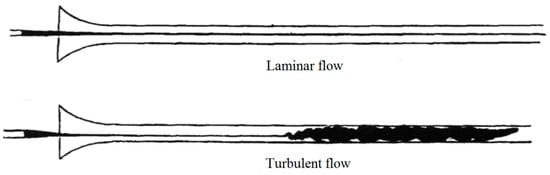
Figure 4.
Representation of turbulent and laminar flow in the original 1883 paper by O. Reynolds [32].
The Sn number is defined by two distinct groups of parameters in the equation shown in Equation (11). The first group involves physical and geometric properties of the flow field, such as ρ, μ, R, and U, which also appear in the Re number. The second group consists of the friction factor, which is not present in the Re number. The friction factor differs for laminar and turbulent flows. In laminar flow, it follows a theoretically determined relationship, while in turbulent flow, it is derived from empirical data. As a result, the friction factor reflects both the knowledge and uncertainties of the empirical database and fitting method. For instance, in Figure 2 and Figure 5, Sn is calculated using a friction factor from Refs. [27,28]. The uncertainties regarding the onset and intensity of turbulence in the transition region have been thoroughly studied through analytical and experimental approaches since the time of Reynolds. The friction factor used in this work is just one of approximately 50 found in the literature. Improved measurement techniques have renewed interest in this issue; the examples of such studies are presented in [33,34]. The growing use of computational fluid dynamics (CFD) for flow simulation allows for the calculation of shear at the wall directly from simulated velocity gradients, thereby transforming the Shear number into a readily utilized parameter for flow regime assessment.
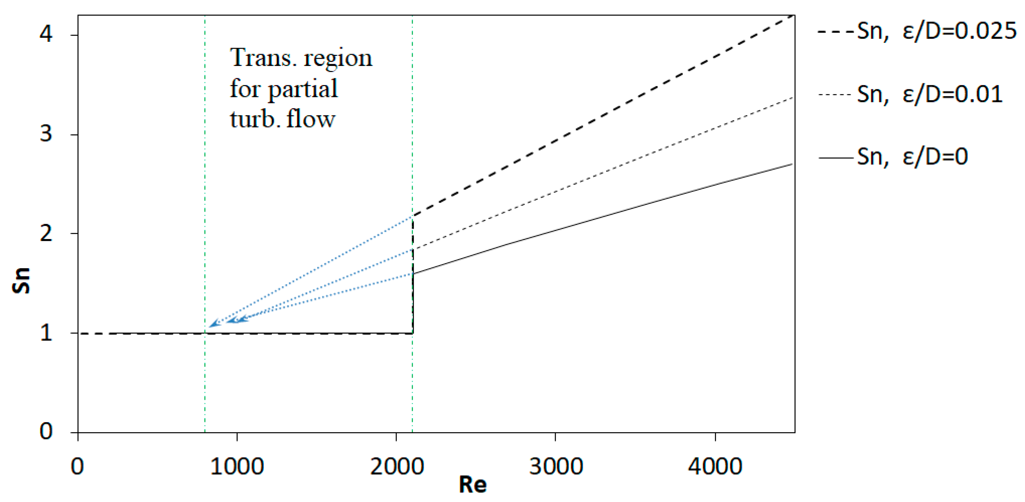
Figure 5.
Turbulent flow transition regions for the Sn.
Using the Sn number as a turbulence indicator in lieu of the Re number does not remove the inherent uncertainties. This is shown by the “Transition region for partial turbulent flow” marked in Figure 5.
Referring to Figure 4, Reynolds noted that turbulence does not appear instantaneously. Somewhere in the pipe, it is initiated and eventually spreads throughout the flow field. This behavior is reflected in the trend of the Sn number. Before the jump in the Sn number shown in Figure 5, turbulence is caused by shear forces near the boundaries but dissipates before reaching the center of the pipe. To assess the Sn number in this transition region, a local effective friction factor is needed. Although it is generally not available, approximate values can be derived by extrapolating trends from existing databases, as illustrated by the blue lines in Figure 5. This illustrates two advantages of the Sn number. First, it relies on the physical mechanism that initiates turbulence and can be used to predict when and where this initiation occurs. Second, the friction factor employed in evaluating the Sn number reflects the state of knowledge represented by a specific database. To enhance the predictive accuracy of the Sn, it is necessary to improve this state of knowledge. However, by employing CFD tools, the shear at the wall can be directly estimated from simulated velocity gradients. This, in turn, allows for the straightforward identification of the transition region using Sn as a quantitative indicator of the flow regime.
6. Conclusions
The Shear number (Sn) is a useful alternative to the Reynolds number (Re) for understanding and predicting turbulent flow. It is especially beneficial in scenarios with different boundaries and two-phase flows. By focusing on the physical causes of flow transitions, Sn simplifies the teaching of turbulence, making it a valuable tool for both educational and practical applications.
The Sn number excels as an indicator of turbulence initiation and development. Since it is derived from the physical mechanisms that trigger turbulence, it provides more precise predictions about when and where turbulence will occur. Additionally, the friction factor in Sn calculations is determined based on specific databases, meaning that as these databases improve, so does the predictive accuracy of the Sn number.
In certain contexts, the Sn number demonstrates greater versatility. It does not solely rely on average fluid velocity and can account for variations in turbulence intensity due to factors like surface roughness or velocity differences at interfaces. These capabilities are particularly advantageous in two-phase or microchannel flows, where the onset of turbulence occurs significantly earlier than would be predicted by the Reynolds number.
Beyond indicating the onset of turbulence, the Sn number also provides a deeper physical explanation of the transition process. In laminar flow, turbulence-generating shear forces and turbulence-dissipating viscous forces are balanced, giving Sn a meaningful value of 1. Turbulence emerges when shear forces exceed the damping ability of molecular viscosity, causing Sn to exceed 1.
While Sn offers clearer explanations and improved predictive capabilities, uncertainties about the initiation and intensity of turbulence remain. Databases of empirical friction coefficients should be refined to increase the accuracy of Sn calculations. However, CFD tools can effectively use Sn as a quantitative indicator of the flow regime, as the shear at the wall can be directly estimated from the simulated velocity gradients. This approach is particularly useful in complex flow optimization analyses.
Author Contributions
Conceptualization, K.A., S.G., M.Š. and R.P.; Methodology, K.A.; Writing—Original Draft, K.A. and S.G.; Validation, S.G.; Data Curation, S.G.; Visualization, S.G.; Writing—Review and Editing, M.Š. and R.P. All authors have read and agreed to the published version of the manuscript.
Funding
This research received no external funding.
Data Availability Statement
The original contributions presented in this study are included in the article. Further inquiries can be directed to the corresponding author.
Conflicts of Interest
The authors declare no conflicts of interest.
Nomenclature
| A | area [m] |
| D | diameter of the channel [m] |
| f | friction factor (by Fanning) |
| L | characteristic linear dimension [m] |
| N | Boundary layer number |
| P | perimeter of cross-section [m] |
| r, R | radius of the channel [m] |
| Req | equivalent radius (1/2 Deq) [m] |
| Re | Reynolds number |
| Sn | Shear number |
| u | velocity component in the flow field [m/s] |
| U | velocity [m/s] |
| U∞ | velocity far from the boundary layer [m/s] |
| V | volume of the fluid element [m3] |
| x | axial coordinate |
| y | vertical coordinate |
| y+ | nondimensional distance away from the wall in a normal direction |
| δ | thickness of the boundary layer [m] |
| ε | measure of the roughness of the pipe wall |
| τ | shear stress [Pa] |
| ρ | density [kg/m3] |
| μ | dynamic viscosity [Pa·s] |
| Subscripts | |
| av | average |
| g | gas |
| in | interface |
| j | jth wall |
| l | liquid |
| sh | shear |
| vi | viscous |
| w | wall |
References
- Feynman, R. The Feynman Lectures on Physics; Addison-Wesley: Boston, MA, USA, 1964. [Google Scholar]
- Eckhardt, B. Transition to turbulence in shear flows. Phys. A Stat. Mech. App. 2018, 504, 121–129. [Google Scholar] [CrossRef]
- Wygnanski, I.J.; Champagne, F.H. On transition in a pipe. Part 1. The origin of puffs and slugs and the flow in a turbulent slug. J. Fluid Mech. 1973, 59, 281. [Google Scholar] [CrossRef]
- Wygnanski, I.J.; Sokolov, M.; Friedman, D. On transition in a pipe. Part 2. The equilibrium puff. J. Fluid Mech. 1975, 69, 283. [Google Scholar] [CrossRef]
- Leonard, A.; Reynolds, W.C. Turbulence research by numerical simulation. In Perspectives in Fluid Mechanics, Proceedings of a Symposium Held on the Occasion of the 70th Birthday of Hans Wolfgang Liepmann, Pasadena, CA, USA, 10–12 January 1985; Lecture Notes in Physics; Springer: Berlin, Germany, 1985; Volume 320, pp. 113–142. [Google Scholar]
- O’Sullivan, P.L.; Breuer, K.S. Transient growth in a circular pipe flow. II Nonlinear development. Phys. Fluids 1994, 6, 3652. [Google Scholar] [CrossRef]
- Nikitin, N.V. Direct numerical modeling of three-dimensional turbulent flows in pipes of circular cross section. Fluid Dyn. 1994, 29, 749. [Google Scholar] [CrossRef]
- Priymak, V.G.; Miyazaki, T. Accurate Navier–Stokes investigation of transitional and turbulent flows in a circular pipe. J. Comput. Phys. 1998, 142, 370. [Google Scholar] [CrossRef]
- Shan, H.; Ma, B.; Zhang, Z.; Nieuwstadt, F.T.M. Direct numerical simulation of a puff and a slug in transitional cylindrical pipe flow. J. Fluid Mech. 1999, 387, 39. [Google Scholar] [CrossRef]
- Reuter, J.; Rempfer, D. Analysis of pipe flow transition. Part 1. Direct numerical simulation. Theor. Comput. Fluid Dyn. 2004, 17, 273. [Google Scholar] [CrossRef]
- Darbyshire, A.G.; Mullin, T. Transition to turbulence in constant-mass-flux pipe flow. J. Fluid Mech. 1995, 289, 83. [Google Scholar] [CrossRef]
- Draad, A.A.; Kuiken, G.D.C.; Nieuwstadt, F.T.M. Laminar-turbulent transition in pipe flow for Newtonian and non-Newtonian fluids. J. Fluid Mech. 1998, 377, 267. [Google Scholar] [CrossRef]
- Jimenez, J.; Moin, P. The minimal flow unit in near-wall turbulence. J. Fluid Mech. 1991, 225, 213. [Google Scholar] [CrossRef]
- Waleffe, F. Three-dimensional coherent states in plane shear flows. Phys. Rev. Lett. 1998, 81, 4140. [Google Scholar] [CrossRef]
- Waleffe, F. Exact coherent structures in channel flow. J. Fluid Mech. 2001, 435, 93. [Google Scholar] [CrossRef]
- Waleffe, F. Homotopy of exact coherent structures in plane shear flows. Phys. Fluids 2003, 15, 1517–1534. [Google Scholar] [CrossRef]
- Gasiūnas, S.; Seporaitis, M.; Almenas, K. Turbulence predicting criterion based on shear forces at the boundaries in a two-phase flow. Int. J. Therm. Sci. 2019, 135, 61–71. [Google Scholar] [CrossRef]
- Laurinavicius, D.; Seporaitis, M. Initiation of Water Turbulence in Concurrent Two-phase Flow. In Facile Preparation of Concentrated Silver and Copper Heat Transfer Nanocolloids, Proceedings of the 12th International Conference on Heat Transfer, Fluid Mechanics and Thermodynamics (HEFAT 2016), Costa del Sol, Spain, 11–13 July 2016; American Society of Thermal and Fluids Engineers: Danbury, CT, USA, 2016; ISBN 978-1-77592-124-0. [Google Scholar]
- Liu, C.; Yan, Y.; Lu, P. Physics of turbulence generation and sustenance in a boundary layer. Comput. Fluids 2014, 102, 353–384. [Google Scholar] [CrossRef]
- Kim, J.; Moin, P.; Moser, R. Turbulence statistics in fully developed channels flows at low Reynolds numbers. J. Fluid Mech. 1987, 177, 133–166. [Google Scholar] [CrossRef]
- Ahn, J.; Lee, J.H.; Jang, S.J.; Hyung, J.S. Direct numerical simulations of fully developed turbulent pipe flows for Reτ = 180, 544 and 934. Int. J. Heat Fluid Flow 2013, 44, 222–228. [Google Scholar] [CrossRef]
- Tsukahara, T.; Seki, Y.; Kawamura, H.; Tochio, D. DNS of turbulent channel flow at very low Reynolds numbers. In Proceedings of the 4th International Symposium on Turbulence and Shear Flow Phenomena, Williamsburg, VA, USA, 27–29 June 2005; pp. 935–940. [Google Scholar]
- Wu, X.; Moin, P. Direct numerical simulation of turbulence in a nominally zero-pressure-gradient flat-plate boundary layer. J. Fluid Mech. 2009, 630, 5–41. [Google Scholar] [CrossRef]
- Duggleby, A.; Ball, K.S.; Schwaenen, M. Structure and dynamics of low Reynolds number turbulent pipe flow. Phil. Trans. R. Soc. A. 2009, 367, 473–488. [Google Scholar] [CrossRef]
- Schlichting, H.; Gersten, K. Boundary-Layer Theory; Springer: Berlin/Heidelberg, Germany, 2000; ISBN 3-540-66270-7. [Google Scholar]
- Kuneš, J. Dimensionless Physical Quantities in Science and Engineering; Elsevier: Cambridge, MA, USA, 2012. [Google Scholar]
- Fanning, J.T. A Practical Treatise on Hydraulic and Water-Supply Engineering; Van Nostrand, D., Ed.; Nabu Press: New York, NY, USA, 1896; ISBN 978-5-87581-042-8. [Google Scholar]
- Colebrook, C.F. Turbulent Flow in Pipes, with Particular Reference to the Transition Region between the Smooth and Rough Pipe Laws. J. Inst. Civ. Eng. 1939, 11, 133–156. [Google Scholar] [CrossRef]
- Berselli, L.C.; Iliescu, T.; Layton, W.J. Mathematics of Large Eddy Simulation of Turbulent Flows; Springer: Berlin/Heidelberg, Germany, 2006. [Google Scholar] [CrossRef]
- Kolmogorov, A.N. Dissipation of energy under locally isotropic turbulence. Proc. R. Soc. Lond. 1991, 434, 15–17. [Google Scholar] [CrossRef]
- Rory, C.; Chien-chia, L.; Gustavo, G.; Pinaki, C. Small-scale universality in the spectral structure of transitional pipe flows. Sci. Adv. 2020, 6, eaaw6256. [Google Scholar] [CrossRef]
- Reynolds, O. An experimental investigation of the circumstances which determine whether the motion of water shall be direct or sinuous, and of the law of resistance in parallel channels. Philos. Trans. 1883, 174, 935–982. [Google Scholar]
- Taylor, J.B.; Carrano, A.; Kandlikar, S.G. Characterization of the effect of surface roughness and texture on fluid flow—Past, present and future. Int. J. Therm. Sci. 2006, 45, 962–968. [Google Scholar] [CrossRef]
- Allen, J.J.; Shockling, M.A.; Kunkel, G.J.; Smits, A.J. Turbulent flow in smooth and rough pipes. Phil. Trans. R. Soc. A. 2007, 365, 699–714. [Google Scholar] [CrossRef]

Disclaimer/Publisher’s Note: The statements, opinions and data contained in all publications are solely those of the individual author(s) and contributor(s) and not of MDPI and/or the editor(s). MDPI and/or the editor(s) disclaim responsibility for any injury to people or property resulting from any ideas, methods, instructions or products referred to in the content. |
© 2025 by the authors. Licensee MDPI, Basel, Switzerland. This article is an open access article distributed under the terms and conditions of the Creative Commons Attribution (CC BY) license (https://creativecommons.org/licenses/by/4.0/).