Figure 1.
Ventilation tunnel laboratory model. (a) Actual tunnel model of Zijin Mining, located in Shanxi province; (b) physical model of three-center arch sections; (c) physical model of tunnel; (d) schematic of smooth model; and (e) schematic of rough model.
Figure 1.
Ventilation tunnel laboratory model. (a) Actual tunnel model of Zijin Mining, located in Shanxi province; (b) physical model of three-center arch sections; (c) physical model of tunnel; (d) schematic of smooth model; and (e) schematic of rough model.
Figure 2.
Results of mesh independence verification: (a) smooth model and (b) rough model.
Figure 2.
Results of mesh independence verification: (a) smooth model and (b) rough model.
Figure 3.
Physical model of Ding’s experiments.
Figure 3.
Physical model of Ding’s experiments.
Figure 4.
Results of model validation.
Figure 4.
Results of model validation.
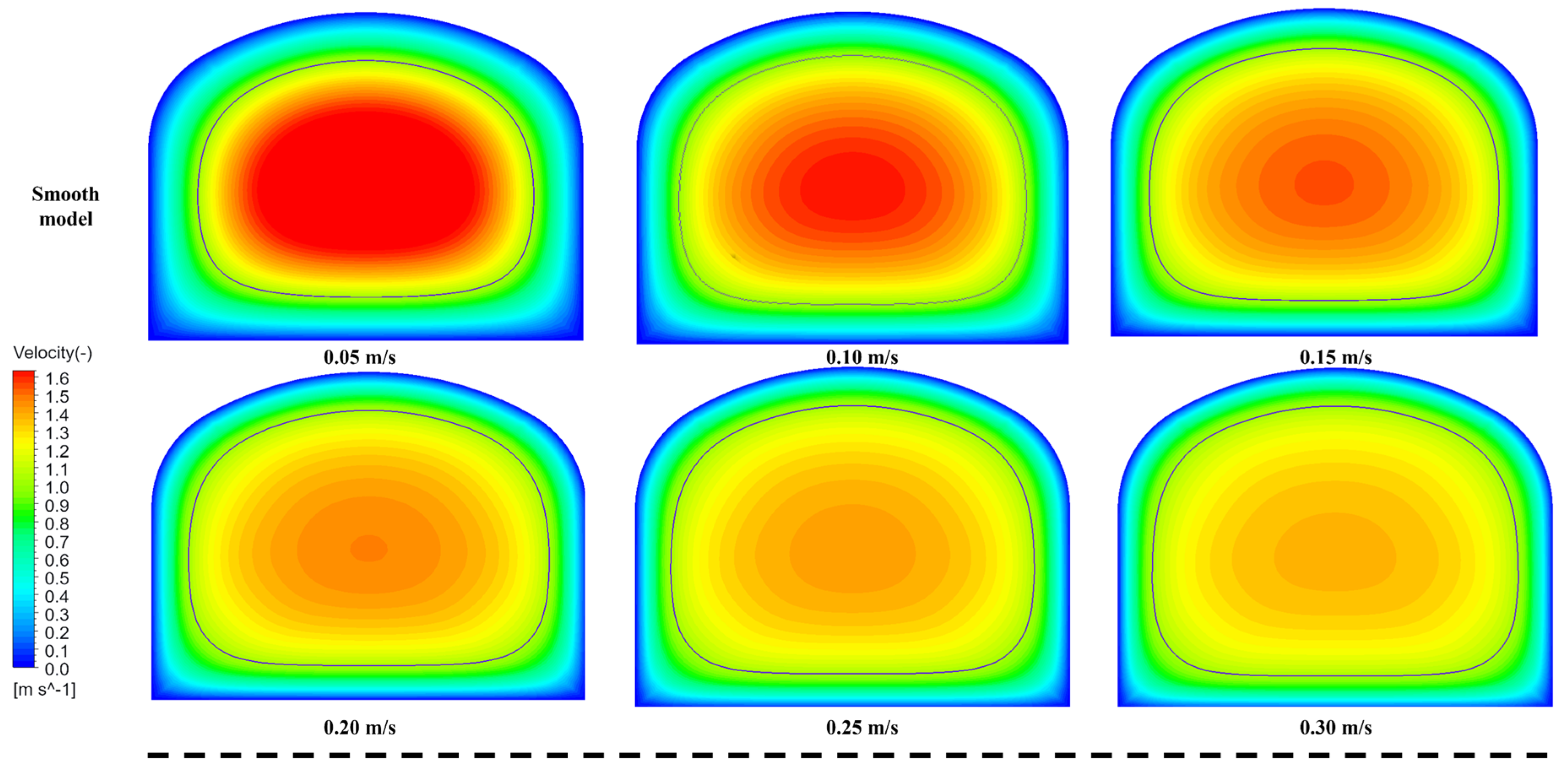
Figure 5.
Dimensionless velocity distribution under laminar regime (1 ).
Figure 5.
Dimensionless velocity distribution under laminar regime (1 ).
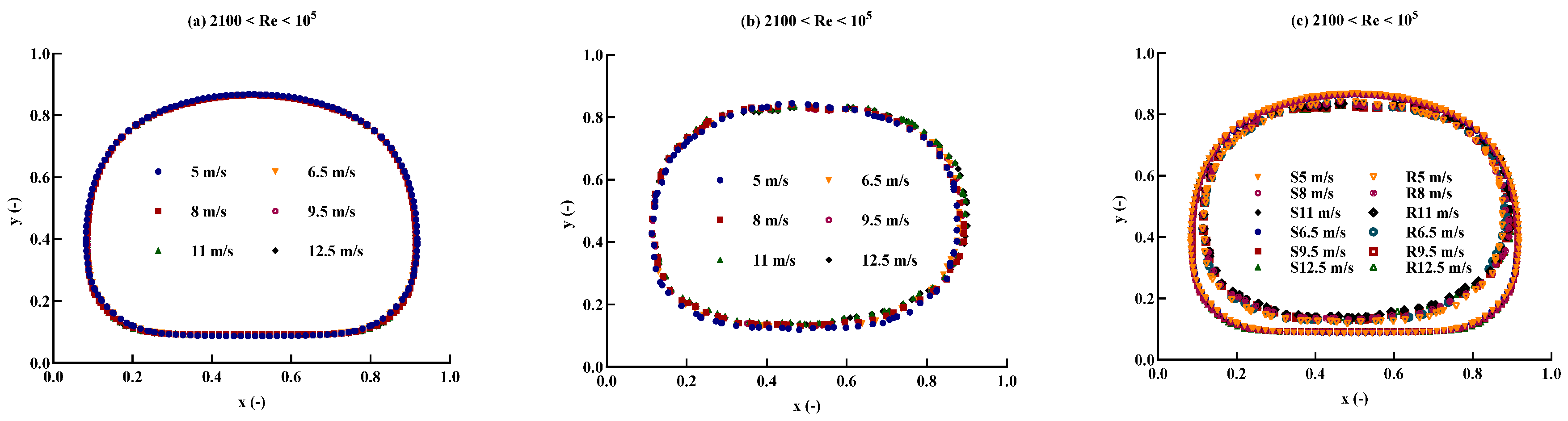
Figure 6.
Dimensionless average velocity distribution under laminar regime. (a) Smooth model, (b) rough model, and (c) their comparisons (S: smooth model, R: rough model).
Figure 6.
Dimensionless average velocity distribution under laminar regime. (a) Smooth model, (b) rough model, and (c) their comparisons (S: smooth model, R: rough model).
Figure 7.
Dimensionless velocity distribution of central velocity field at three-centered arch cross-section. (a) Smooth model, (b) rough model, and (c) their comparisons (S: smooth model, R: rough model).
Figure 7.
Dimensionless velocity distribution of central velocity field at three-centered arch cross-section. (a) Smooth model, (b) rough model, and (c) their comparisons (S: smooth model, R: rough model).
Figure 8.
Dimensionless velocity distribution under transition regime.
Figure 8.
Dimensionless velocity distribution under transition regime.
Figure 9.
Dimensionless average velocity distribution under transition regime. (a) Smooth model, (b) rough model, and (c) their comparisons (S: smooth model, R: rough model).
Figure 9.
Dimensionless average velocity distribution under transition regime. (a) Smooth model, (b) rough model, and (c) their comparisons (S: smooth model, R: rough model).
Figure 10.
Dimensionless velocity distribution of central velocity field at three-centered arch cross-section under transition regime. (a) Smooth model, (b) rough model, and (c) their comparisons (S: smooth model, R: rough model).
Figure 10.
Dimensionless velocity distribution of central velocity field at three-centered arch cross-section under transition regime. (a) Smooth model, (b) rough model, and (c) their comparisons (S: smooth model, R: rough model).
Figure 11.
Dimensionless velocity distribution under fully developed turbulence regime.
Figure 11.
Dimensionless velocity distribution under fully developed turbulence regime.
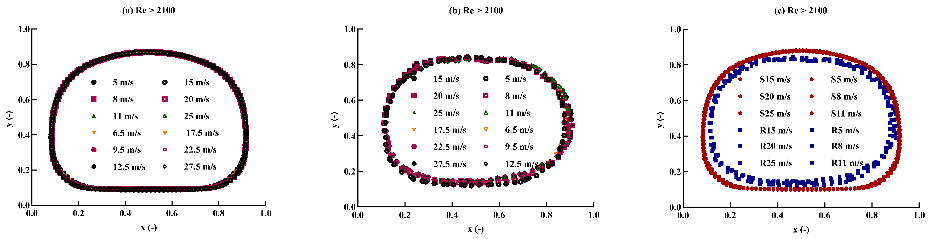
Figure 12.
Dimensionless average velocity distribution under fully developed turbulence regime. (a) Smooth model, (b) rough model, and (c) their comparisons (S: smooth model, R: rough model).
Figure 12.
Dimensionless average velocity distribution under fully developed turbulence regime. (a) Smooth model, (b) rough model, and (c) their comparisons (S: smooth model, R: rough model).
Figure 13.
Dimensionless velocity distribution of central velocity field at three-centered arch cross-section under fully developed turbulence regime. (a) Smooth model, (b) rough model, and (c) their comparisons (S: smooth model, R: rough model).
Figure 13.
Dimensionless velocity distribution of central velocity field at three-centered arch cross-section under fully developed turbulence regime. (a) Smooth model, (b) rough model, and (c) their comparisons (S: smooth model, R: rough model).
Figure 14.
Dimensionless average velocity distribution under turbulence regime. (a) Smooth model, (b) rough model, and (c) their comparisons (S: smooth model, R: rough model).
Figure 14.
Dimensionless average velocity distribution under turbulence regime. (a) Smooth model, (b) rough model, and (c) their comparisons (S: smooth model, R: rough model).
Figure 15.
Dimensionless velocity distribution of central velocity field at three-centered arch cross-section under turbulence regime. (a) Smooth model, (b) rough model, and (c) their comparisons (S: smooth model, R: rough model).
Figure 15.
Dimensionless velocity distribution of central velocity field at three-centered arch cross-section under turbulence regime. (a) Smooth model, (b) rough model, and (c) their comparisons (S: smooth model, R: rough model).
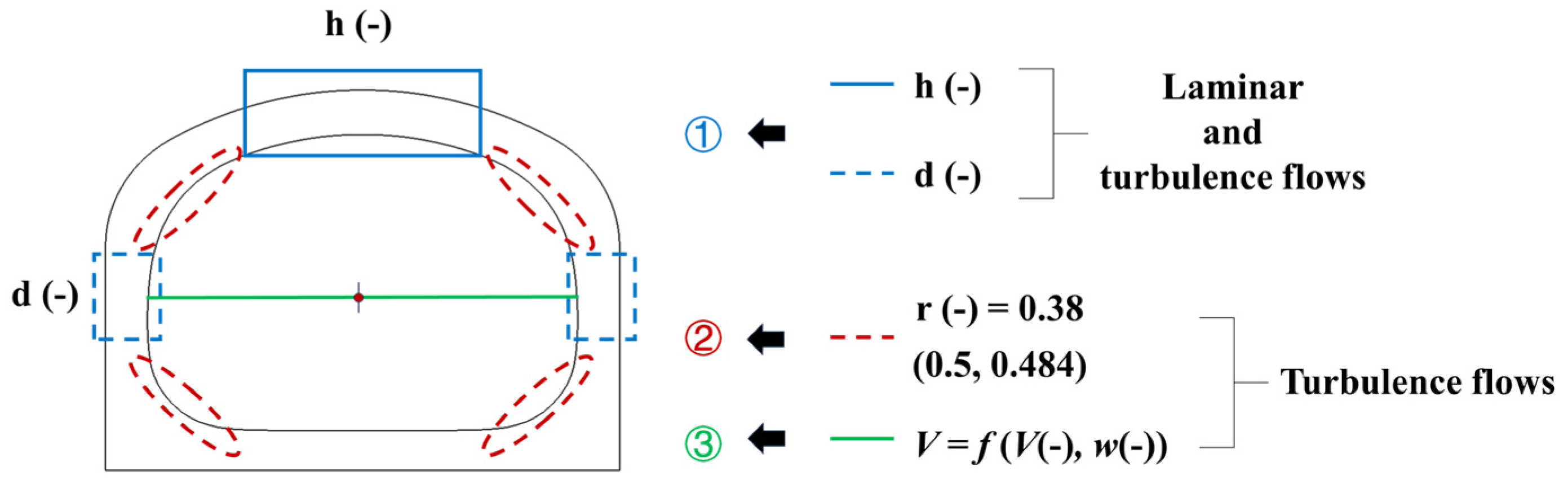
Figure 16.
Schematic of dimensionless average velocity ring with dimensionless cross-section. (The blue arrow represents , and the red one represents ).
Figure 16.
Schematic of dimensionless average velocity ring with dimensionless cross-section. (The blue arrow represents , and the red one represents ).
Figure 17.
distribution under different flow regimes. (a) Laminar regime, (b) transition regime, (c) fully developed turbulence regime, and (d) turbulence regime.
Figure 17.
distribution under different flow regimes. (a) Laminar regime, (b) transition regime, (c) fully developed turbulence regime, and (d) turbulence regime.
Figure 18.
distribution under different flow regimes. (a) Laminar regime, (b) transition regime, (c) fully developed turbulence regime, and (d) turbulence regime.
Figure 18.
distribution under different flow regimes. (a) Laminar regime, (b) transition regime, (c) fully developed turbulence regime, and (d) turbulence regime.
Figure 19.
Results of data fitting based on fitting model.
Figure 19.
Results of data fitting based on fitting model.
Figure 20.
Linear fit of and velocity.
Figure 20.
Linear fit of and velocity.
Figure 21.
Second-order polynomial fit of and velocity.
Figure 21.
Second-order polynomial fit of and velocity.
Figure 22.
The establishment of the installation location for the airflow measurement apparatus.
Figure 22.
The establishment of the installation location for the airflow measurement apparatus.
Table 1.
Operating conditions of three-center section tunnel.
Table 1.
Operating conditions of three-center section tunnel.
| Parameters | Value/Scheme | Comment |
|---|
| Inlet velocity/(m/s) | 0.05, 0.10, 0.15, 0.20, 0.25, 0.30 | 1 < Re < 2100 |
| 5.0, 6.5, 8.0, 9.5, 11.0, 12.5, | 2100 < Re < 105 |
| 15.0, 17.5, 20.0, 22.5, 25.0, 27.5 | 105 < Re |
| Outlet relative pressure/Pa | 0 | |
| Wall | No slip | |
| Wall function | Enhanced wall function | |
| Segregated algorithm | PISO | |
| Airflow iterations | 2500 | |
| Time step size | 10−5 | |
| Gradient solver scheme | Least Squares Cell-based Method | |
| Momentum and turbulence solver scheme | Second-Order Upwind | |
| Pressure solver scheme | PRESTO! | |
Table 2.
Geometric and operating conditions of three-center section tunnel.
Table 2.
Geometric and operating conditions of three-center section tunnel.
| Parameters | Value/Scheme |
|---|
| Large arch radius/mm | 366 |
| Small arch radius/mm | 132 |
| Width/mm | 520 |
| Wall height/mm | 226 |
| Length/m | 16 |
| Temperature/°C | 15 |
| Viscosity/(m2/s) | 14.4 × 10⁻⁶ |
| 1.44 |
| 1.92 |
| 0.09 |
| 1.0 |
| 0.85 |
Table 3.
R2 for different scale models (without considering heat transfer process).
Table 3.
R2 for different scale models (without considering heat transfer process).
| Model Scale | R2 of Smooth Models | R2 of Rough Models |
|---|
| 1 | 1.000 | 1.000 |
| 2 | 0.977 | 0.919 |
| 4 | 0.953 | 0.925 |
| 8 | 0.965 | 0.922 |
| 10 | 0.959 | 0.919 |
Table 4.
R2 for different scale and temperature models.
Table 4.
R2 for different scale and temperature models.
| Model Scale | R2 of Smooth Models/Rough Models |
|---|
| | 15 °C | 20°C | 25 °C | 30 °C | 35 °C |
| 1 | 0.993/0.956 | 0.981/0.945 | 0.982/0.951 | 0.976/0.944 | 0.973/0.939 |
| 2 | 0.966/0.944 | 0.969/0.935 | 0.970/0.939 | 0.958/0.940 | 0.959/0.935 |
| 4 | 0.959/0.938 | 0.951/0.932 | 0.950/0.932 | 0.949/0.942 | 0.949/0.939 |
| 8 | 0.960/0.933 | 0.952/0.933 | 0.949/0.935 | 0.959/0.940 | 0.946/0.930 |
| 10 | 0.946/0.932 | 0.944/0.930 | 0.941/0.932 | 0.949/0.938 | 0.945/0.929 |
Table 5.
R2 for different turbulence models.
Table 5.
R2 for different turbulence models.
| Model Scale | R2 of Smooth Models/Rough Models |
|---|
| | | | | Spalart–Allmaras | LES |
|---|
| 1 | 1.000/1.000 | 0.991/0.992 | 0.992/0.991 | 0.893/0.886 | 0.990/0.992 |
| 2 | 0.977/0.919 | 0.972/0.918 | 0.970/0.910 | 0.850/0.831 | 0.979/0.955 |
| 4 | 0.953/0.953 | 0.955/0.951 | 0.945/0.946 | 0.802/0.806 | 0.969/0.946 |
| 8 | 0.965/0.922 | 0.963/0.933 | 0.960/0.922 | 0.801/0.803 | 0.959/0.936 |
| 10 | 0.959/0.919 | 0.962/0.923 | 0.951/0.912 | 0.773/0.765 | 0.963/0.931 |
Table 6.
The distribution of the dimensionless vertical coordinates of the velocity cores under different velocities.
Table 6.
The distribution of the dimensionless vertical coordinates of the velocity cores under different velocities.
| Partition | Velocity (m/s) | of Smooth Models | of Rough Models | of Smooth Models | of Rough Models |
|---|
| Laminar regime | 0.05 | 0.469 | 0.486 | 0.453 | 0.467 |
| 0.10 | 0.459 | 0.471 |
| 0.15 | 0.454 | 0.476 |
| 0.20 | 0.448 | 0.466 |
| 0.25 | 0.448 | 0.456 |
| 0.30 | 0.438 | 0.446 |
| Transition regime | 5.0 | 0.474 | 0.481 | 0.462 | 0.484 |
| 6.5 | 0.464 | 0.486 |
| 8.0 | 0.448 | 0.486 |
| 9.5 | 0.469 | 0.486 |
| 11.0 | 0.454 | 0.481 |
| 12.5 | 0.464 | 0.486 |
| Fully developed turbulence regime | 15.0 | 0.464 | 0.476 | 0.468 | 0.484 |
| 17.5 | 0.474 | 0.481 |
| 20.0 | 0.469 | 0.481 |
| 22.5 | 0.469 | 0.486 |
| 25.0 | 0.470 | 0.491 |
| 27.5 | 0.459 | 0.486 |
Table 7.
Dimensions of three-center arch tunnels of Ding’s models.
Table 7.
Dimensions of three-center arch tunnels of Ding’s models.
| Large Arch Radius/mm | Small Arch Radius/mm | Width/mm | Wall Height/mm | Length/m |
|---|
| 183 | 66 | 260 | 113 | 8 |
| 366 | 132 | 520 | 226 | 16 |
| 549 | 198 | 780 | 339 | 24 |
| 732 | 264 | 1040 | 452 | 32 |
| 915 | 330 | 1300 | 565 | 40 |
Table 8.
Results of data fitting based on fitting model.
Table 8.
Results of data fitting based on fitting model.
| Velocity/(m/s) | | | |
|---|
| 5.0 | 1.224 | 0.0209 | 0.984 |
| 6.5 | 1.219 | 0.0188 | 0.985 |
| 8.0 | 1.220 | 0.0182 | 0.986 |
| 9.5 | 1.218 | 0.0177 | 0.988 |
| 11.0 | 1.212 | 0.0166 | 0.989 |
| 12.5 | 1.210 | 0.0157 | 0.990 |
| 15.0 | 1.200 | 0.0143 | 0.992 |
| 17.5 | 1.195 | 0.0141 | 0.990 |
| 20.0 | 1.186 | 0.0133 | 0.991 |
| 22.5 | 1.185 | 0.0133 | 0.990 |
| 25.0 | 1.180 | 0.0125 | 0.992 |
| 27.5 | 1.179 | 0.0124 | 0.991 |


