Performance of a Pharmaceutical Single-Use Stirred Tank Operating at Different Filling Volumes: Mixing Time, Fluid Dynamics and Power Consumption

Abstract

Single-use bioreactors (SUBs) are revolutionizing biotechnology and biopharmaceutical manufacturing by offering cost-efficient, flexible, and scalable alternatives to traditional reusable systems. These bioreactors, made from disposable and pre-sterilized materials, streamline cell cultivation for biological production while minimizing the need for complex cleaning and sterilization. A critical aspect of SUB performance lies in optimizing hydrodynamic parameters flow field, power consumption, mixing time, and energy efficiency, which directly influence process outcomes. This study investigates the hydrodynamic performance of an SUB system through stereo Particle Image Velocimetry (PIV) to analyze flow fields, Planar Laser-Induced Fluorescence (PLIF) for mixing time, and Electro Resistance Tomography (ERT) for further insights into mixing dynamics. The results, evaluated at varying impeller speeds and fill heights, provide a comprehensive understanding of flow behavior, mixing efficiency, and power requirements. This work highlights the importance of hydrodynamic characterization in optimizing SUB design and operation, contributing to more sustainable and efficient biopharmaceutical production.

1. Introduction

Single-use bioreactors (SUBs) represent a transformative innovation in biotechnology and biopharmaceutical manufacturing [1]. These systems are designed for single use, eliminating the need for the complex cleaning and sterilization associated with traditional reusable bioreactors. SUBs are primarily employed in the cultivation of cells to produce biopharmaceuticals, vaccines, and other biologics, offering significant advantages in terms of cost-efficiency, flexibility, and speed [2,3]. The growing demand for biologics has driven the need for more adaptable and scalable production methods [4]. Single-use systems are particularly beneficial in small to medium-scale operations, providing rapid deployment and reduced capital investment compared to traditional stainless-steel bioreactors. These bioreactors are made from disposable, pre-sterilized materials such as plastic bags and flexible tubing, designed to handle the complex and sensitive nature of biological processes. In addition to cost and time savings, SUBs contribute to enhanced product quality and the reduced risk of cross-contamination, as each batch is produced in a closed, single-use environment. These systems can be easily integrated into continuous manufacturing processes, offering a more sustainable approach to biomanufacturing. As the biotechnology industry continues to evolve, SUBs are poised to play a crucial role in streamlining production and advancing the development of life-saving biologics.

Hydrodynamic parameters, including flow field, power consumption, mixing time, and mixing energy, are crucial for describing the functionality and efficiency of bioreactors. Optimizing hydrodynamic conditions maximizes the yield of desired products. Power consumption measurements in stirred tank bioreactors are essential for optimizing bioprocesses, improving efficiency, and ensuring cost-effectiveness in industrial-scale bioprocessing. Power consumption provides direct insight into the efficiency of mixing within the bioreactor [5]. By monitoring the power required for stirring, operators can assess whether the mixing is adequate for cell growth or product formation. Over-mixing or under-mixing can lead to suboptimal growth conditions, affecting yield and product quality. Optimizing power usage leads to a more homogeneous environment for cells, improving process consistency and product quality, and is often used as a critical input parameter for scale-up [6]. Variations in power usage may signal changes in parameters like viscosity, cell density, or media composition, directly influencing metabolic activity rates or bioreactor efficiency. For example, higher than expected power consumption could indicate increased viscosity due to cell growth or by-product accumulation, prompting early intervention to adjust conditions and avoid process inefficiencies. In large-scale manufacturing, accurate power consumption measurements help scale up laboratory-scale processes to industrial levels. Scaling up typically involves changes in reactor geometry, impeller design, and agitation speed, all affecting power requirements [7,8]. By analyzing power consumption data at smaller scales [6], operators can predict and optimize power usage when moving to larger reactors, ensuring the scaling process does not compromise efficiency or product yield. Power consumption data are also essential for optimizing stirred tank bioreactor design. By analyzing how different designs (e.g., impeller type, size, and configuration) affect power usage, engineers can develop more efficient bioreactor systems [6]. This leads to better-performing reactors with lower energy consumption, beneficial both economically and environmentally. Comprehensive engineering characterization of the fluid dynamics in such systems helps understand the changes in flow features affecting power consumption and mixing time [7,9,10,11,12]. In this study, we compare results obtained using stereo PIV (Particle Image Velocimetry) to analyze the flow field of the investigated system. PLIF (Planar Laser-Induced Fluorescence) [13,14] and ERT (Electro Resistance Tomography) [15] were used to investigate the system’s mixing time. The acquired data are compared, and the overall performance of the SUB system, operating at a typical impeller speed and different filling heights, is examined. In this work, one of the single use bioreactor types, the Flexel Levmixer by Sartorius, is investigated.

2. Materials and Methods

2.1. Experimental Rig

In Figure 1a, the schematic of the rig used for this work is shown. A cubic vessel with a volume of 50 L and dimensions matching those of the Flexel Levmixer (square base of 395 mm × 395 mm, T × T, (IV)) was utilized for this study. Key differences from the original vessel include the use of plexiglass for the walls instead of disposable plastic, ensuring optical transparency, and a standard shaft connection to the motor (I) for accurate measurement of impeller power consumption, as opposed to a magnetic levitation system. For agitation, a 3D-printed version of the original impeller (III) with a diameter of 126 mm was installed. The 3D printer used was a Guider IIs (Flashforge, Hangzhou, China). The rig schematic is illustrated in Figure 1a. The motor (I) is linked to a variable frequency driver, enabling precise control of the impeller speed. It connects to the impeller via a detachable shaft, fitted with couplings for integrating the Kistler torque sensor (II) type 4502A0.5HA, which has a measurement range of 0.5 Nm. Detailed information about the theoretical background of the torque measurements and standard operating procedure can be found in the previous work by Alberini et al. [2].

2.2. Stereo-PIV Measurements

Stereo-PIV measurements were conducted in the region identified in Figure 1 (in green), at the bottom side of the vessel. The measurement area is positioned on a vertical plane halfway between the two lateral walls (Z direction) of the vessel. Image acquisition was carried out using two HiSenseMKII digital cameras (1344 × 1024 pixels CCD; Dantec Dynamics, Skovlunde, Denmark) mounted on Scheimpflug adapters. One camera was oriented perpendicular to the laser sheet (θ1), and the other was set at a 20° angle (θ2) relative to the first. Both cameras were equipped with optical filters to minimize ambient light interference. The laser sheet was generated by a pulsed Nd Litron laser (wavelength of 532 nm, frequency of 15 Hz, energy of 65 mJ/pulse), synchronized with the cameras using the Dantec Dynamics “Timer Box” system. Data acquisition and processing were performed using “Dynamics Studio 7.6” software. The same setup was used in the previous work by Alberini et al. [2].

2.3. PLIF Measurements

PLIF (Planar Laser-Induced Fluorescence) measurements were conducted in the region highlighted in Figure 1a,c (shown in purple) to measure the mixing time. The area of interest is located at the bottom side of the vessel, to the same region analyzed using stereo-PIV. The hardware setup for PLIF measurements was identical to that used for stereo-PIV, except for the use of rhodamine 6 G dye instead of seeding particles to monitor concentration changes in the system. The main difference in the setup was the camera filters (green filter, HOYA X1); for PLIF, orange filters (HOYA YA3) were employed (Kenko Tokina Co., Ltd., Tokyo, Japan). Although both cameras recorded data, only images from the frontal camera were used for analysis, as the results from both cameras were identical.

The raw PLIF data consisted of images in which pixel intensity varied according to the concentration of rhodamine 6 G. These images were post-processed using MATLAB 2023b with custom scripts developed in-house.

The experiments utilized a 10 mL syringe containing a concentrated rhodamine 6 G solution at a concentration of 250 mg/L. Injections were performed at the top of the liquid column (adjusted for the liquid height) by inserting the syringe needle 1 cm into the liquid (along the y-axis) to prevent air entry. The x-axis position corresponded to the vessel wall, while the z-axis position for all injections was set at the mid-point of the square base’s side length.

For each condition, three replicate injections were performed at each liquid height. Each injection increased the rhodamine 6 G concentration by approximately 0.05 mg/L, consistent with previous studies [15]. To ensure a linear relationship between rhodamine concentration and pixel intensity (as reported in [16]), water was replaced before the rhodamine concentration exceeded 1 mg/L.

Table 1. Injections volumes used for the different filling level mixing time experiments.

V(L)	H (cm)	R6G (mg)	mL
10.92	7	0.54	2.2
17.16	11	0.85	3.4
29.64	19	1.48	5.9
40.57	26	2.02	8.0
49.93	32	2.49	10.0

summarizes the injection volumes for various liquid heights. The injection volumes were adjusted to maintain a consistent increase in rhodamine concentration for each experiment. Given the volumes were different, zero time was considered when the injection was completed. This was evaluated by counting the images during the recording. Given the recording frequency of 15 Hz, the error is well within one second.

2.4. ERT Measurements

Electro-Resistance Tomography (ERT) measurements were conducted in the region highlighted in Figure 1a,c (shown in orange) to evaluate mixing time. Part of the area of interest overlapped with the region used for PLIF measurements. As will be discussed later, differences in the size of the measurement area can influence transient data but do not affect overall mixing time results. Theoretically, if a high level of mixing is achieved within a given volume, the location of the area of interest within the vessel should not impact the mixing time measurements.

For these experiments, a vertical plane was captured using a linear probe equipped (as shown in Figure 1d) with 16 electrodes and 2 grounding electrodes, with dimensions of 20 mm by 5.5 mm. The probe was connected to an ITS P2000 ERT system from Industrial Tomography Systems Ltd., Manchester, UK. The electrodes were linked to the data acquisition system (DAS) via coaxial cables.

The measurements were performed using the adjacent strategy, where electric current was injected through adjacent pairs of electrodes, and voltage differences were measured across all other electrode pairs. This process was repeated for every independent electrode pair. The injected current was fixed at 15 mA, and the frequency was set at 9600 Hz. Conductivity maps were reconstructed from the measured electric potential data using the linearized, non-iterative Modified Sensitivity Back Projection (MSBP) algorithm implemented in the ITS System p2+V9 software.

The raw ERT data consisted of rectangular conductivity maps, influenced by the electrode arrangement. The spatial resolution on the plane was determined by dividing the 160 conductivity values across horizontal lines, with 10 cells in the radial direction corresponding to the 16 electrodes. The vertical resolution was based on the distance between consecutive electrodes, measured as 5.5 mm, while the horizontal resolution was estimated to be approximately 6 mm, using the approach described by [17]. The ERT measurements utilized a 10 mL syringe containing a concentrated brine solution of approximately 200 g/L. Injections were performed at the top of the liquid column similarly to the PLIF measurement and as the PLIF a fixed increment of salt concentration was employed, hence same injections (same volume) were used.

In Figure 2, for a selected condition where the liquid height is 26 cm and N = 70 rpm, the normalized data are presented, respectively, for PLIF measurement (Figure 2a) and for ERT measurement (Figure 2b). In Figure 2c is an example of how the transient information of the tracer signal can change by just selecting a different area of interest. In this case, we have selected two different areas of a tomogram (full tomogram and bottom quarter) for the same time signal of Figure 2b. A similar trend was also observed for the PLIF measurements.

For the PLIF images, PI corresponds to the average pixel intensity value of the image in the instant in time. For the ERT tomograms, CND corresponds to the average non-dimensional conductivity value of the tomogram in the instant in time. While the normalized PI and CND correspond to general χ_i of Equation (1):

$${\chi }_i={\displaystyle \frac{f\left(i\right)-f\left(0\right)}{f\left(\infty \right)-f\left(0\right)}}$$

(1)

where f(i) is the PI or CND in the time instant i, while f(0) is the average PI or CND value of the image or tomogram before the injection of the Rhodamine 6 G or salt brine. f(∞) is average PI or CND value of the image or tomogram after the system is fully mixed. Both signals have been processed following the same procedure described in the work by Paglianti et al. [18].

The next step of the analysis is based on the Coefficient of Variation (CoV) on the measurement plane, applied for both signals obtained from PLIF and ERT. The CoV of the normalized local conductivity, χ_i(t), is obtained as follows:

$$CoV\left(t\right)=\sqrt{{\displaystyle \frac{\sum _{i=1}^{N_p}{(\frac{{\chi }_i\left(t\right)}{\widetilde{\chi \left(t\right)}}-1)}^2}{Np-1}}}$$

(2)

where Np is the number of pixels/non-dimensional conductivity values per plane.

Subsequently, the normalized CoV_norm can be calculated as follows:

$${CoV}_{Norm}={\displaystyle \frac{CoV\left(t\right)-CoV\left(\infty \right)}{CoV\left(t=0\right)-CoV\left(\infty \right)}}$$

(3)

where CoV(t = 0) is the averaged CoV value before the injection of the tracer, CoV(∞) corresponds to the complete homogenization condition at t = ∞.

Following the approach outlined by Paul et al. [19] in Chapter 4, the 95% mixing time was determined as the point where the base-10 logarithm of the mixing time signal reaches a value of −2.6 and remains below this threshold as showed in Figure 3.

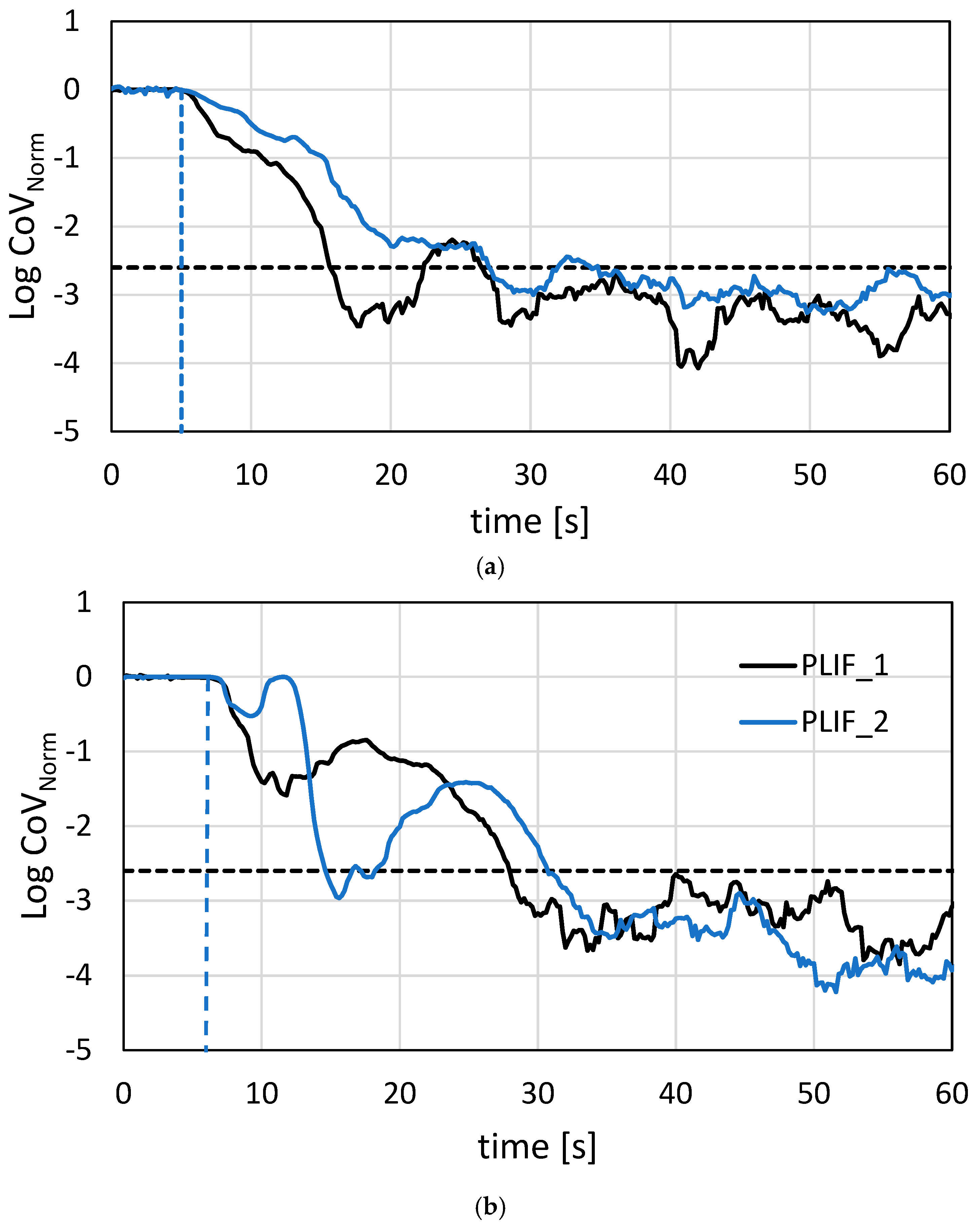
2.5. Repeatability of the PLIF Measurement

Figure 4 illustrates the repeatability of PLIF measurements for three selected liquid heights. Repeatability is evaluated by comparing the difference between the starting point (indicated by vertical dotted lines) and the point where the curves intersect and remain below the horizontal dotted line. This horizontal line represents the threshold for achieving 95% of the mixing time.

As previously noted, achieving identical transient information, even when using the same technique, is challenging. This variability arises primarily from the injection’s starting time, which is not always perfectly synchronized with the impeller’s position relative to the injection point. Nevertheless, the results demonstrate good repeatability across the three reported cases.

To enhance clarity, we have marked the different starting points on the graph. These differences are mainly attributed to the physical time required to initiate the injection. It is worth mentioning that the data recordings (for both PLIF and ERT) were always initiated before the injection began.

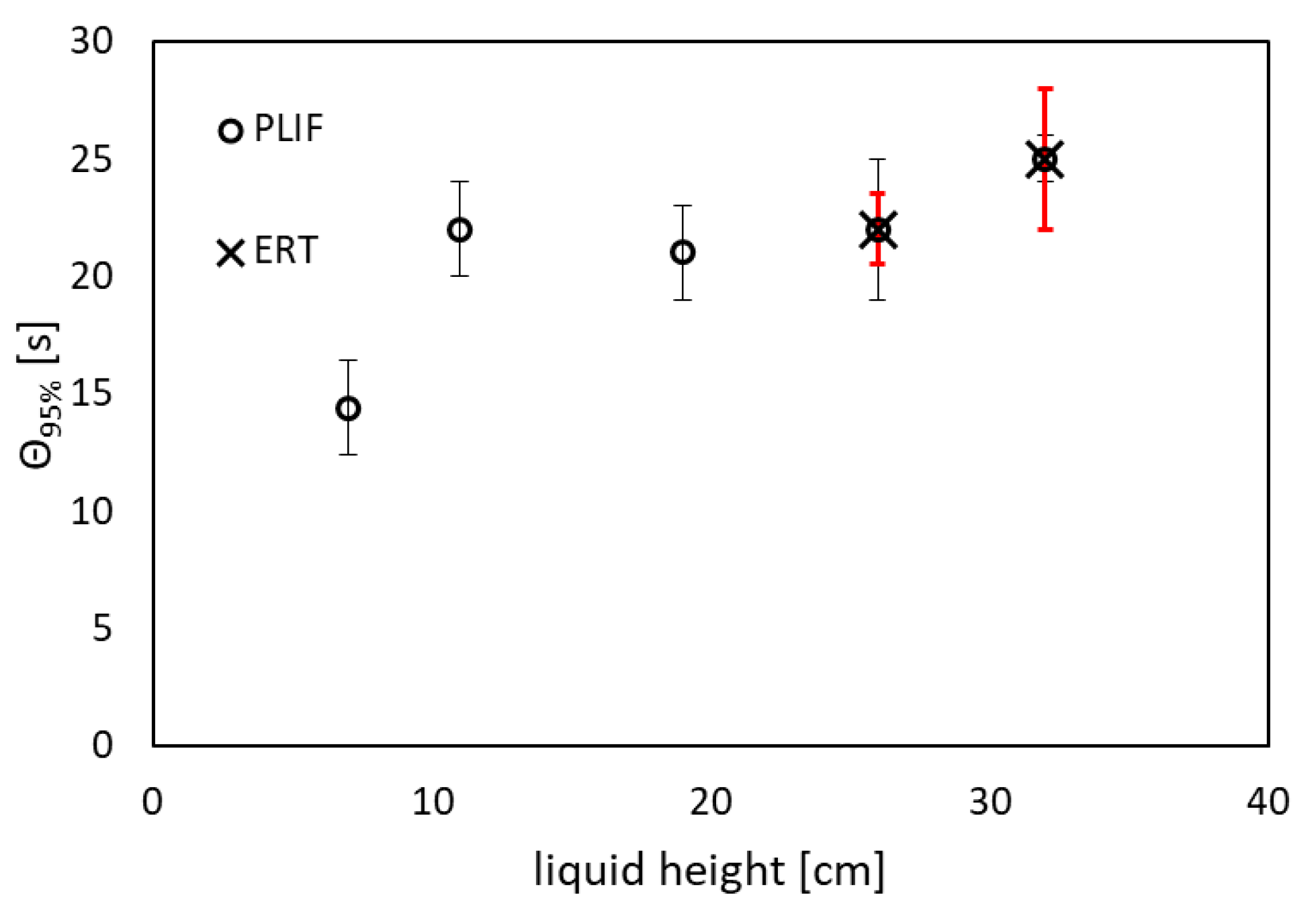
2.6. Congruency Between PLIF and ERT Measurements

The final step in our critical review of the dataset involved directly comparing the mixing time tracers obtained from the two techniques under similar conditions. Similar observations can be made when comparing the transient trends of PLIF and ERT, as illustrated in Figure 5 for liquid heights of 26 cm (a) and 32 cm (b). While the overall mixing time results are consistent between the two techniques, the transient signals show notable differences (as also showed by comparing different injections for the PLIF injections). This is mainly due to the injection timing and relative position of the impeller, which was a variable that could not be controlled. For this work we have evaluated the 95% mixing time; however, we can speculate that 90% mixing time across the different setup and technique showed an overall decrease in the error bar for both techniques, as expected. This comparison reinforces our confidence in the reliability of both techniques, as they produce comparable overall results, making them trustworthy for evaluating mixing time. For the transient mixing time, not only the timing of the injection but also the area of interest plays an important role in the time tracer trend. In fact, changing the area of interest, as shown in Figure 2c, shifted and changed the intensity of the peaks in the transient interval (from the injection to the 95% mixing time).

3. Results

The analysis of the results begins with the power consumption data obtained from torque measurements. Consistent with previous findings from Alberini et al., which were acquired at different impeller speeds, the power number (Po) and power per unit volume (P/V) data as a function of filling height (HL) at a fixed impeller speed of 70 rpm are presented in Figure 6. As previously shown, there is a significant increase in power consumption at the 19 cm filling height, which corresponds roughly to half the length of the base of the square vessel. This increase in power starts from the lower filling level, rises to a maximum, and then both P/V and Po decrease again, stabilizing at similar values for the 26 cm and 32 cm filling levels.

In Figure 7, the plots on the left in each row display the velocity distributions at different filling heights, with a color gradient indicating the intensity of the normalized tangential component (W/Wtip). The vectors represent the radial and tangential components. On the right, each plot presents the same flow field using streamlines, with the velocity vectors representing the radial and axial components, highlighting the flow patterns, direction, and circulation within the field.

In Figure 7a, the lowest filling level is considered. The color gradient reveals a relatively high-velocity region on the left side of the domain, closer to the impeller blade, with the tangential velocity gradually decreasing towards the tank wall. The streamline pattern (Figure 7b) shows complex flow structures, with distinct vortex formations suggesting recirculation zones induced by the interaction between the impeller and the liquid as it is pushed in the tangential direction.

In Figure 7c, the flow at the 11 cm filling level is studied. The color gradient is smoother compared to Figure 7a, with fewer intense gradients, indicating a more developed flow rather than next to the impeller. The streamline map (Figure 7d) here shows a dominant, larger vortex structure, suggesting a major recirculation region.

In Figure 7e, the 19 cm filling level is studied. The color distribution is more uniform than in previous cases, and the overall velocity intensity has changed, with a broad green-to-yellow area indicating a reduction in the tangential component. This suggests a decrease in the solid-body rotation of the fluid. Meanwhile, the other components show an overall increase in intensity, indicating better mixing. The streamline map (Figure 7f) reveals a more organized flow pattern, likely with fewer vortices and a more directional flow.

Figure 7g,i show the flow at the 26 cm and 32 cm filling levels, respectively. The color distributions for these two cases are similar, and as seen in the corresponding streamline maps (Figure 7h,j), the flow structure does not change significantly compared to the previous filling levels.

Finally, Figure 7k shows the distribution of the tangential component for a fixed axial position at Y = 20 mm at different radial positions. Interesting trends can be depicted from the plot. At lower filling levels (7 and 11 cm), the profiles exhibit a declining trend from the impeller tip (on the left side of the plot) towards the tank wall (on the right side of the plot). Meanwhile, for other filling levels, the trend is similar to the ones observed in previous works for the un-baffled stirred tank [20,21,22,23].

Overall, it is evident that the filling height has a significant effect on the structure of vortices and recirculation zones. The presence of vortices in the right-hand plots, especially in the first two rows, highlights areas of recirculation that can both enhance and hinder mixing. While vortices can improve local mixing by circulating the fluid repeatedly, they can also trap portions of fluid, creating dead zones that increase mixing time. In terms of mixing efficiency, the decreasing intensity of the gradients and the evolution of the flow structure from multiple vortices to a more streamlined pattern suggest that mixing efficiency can be significantly affected by changes in the filling height. This analysis shows that the flow patterns significantly influence mixing time, as the flow structure evolves into a more stable pattern with increasing filling height, aiding in a more even distribution of mixing across the domain.

Focusing on the differences in the flow field between the 11 cm and 19 cm filling levels (Figure 7c vs. Figure 7e and Figure 7d vs. Figure 7f), the velocity distributions for all three components are extracted and plotted in Figure 8. In all experiments, the impeller speed is kept constant at N = 70 rpm. From Figure 8a, it is evident that the radial velocity (U) shifts towards higher positive values as the filling level increases from 11 cm to 19 cm. Similarly, for the axial component (V, Figure 8c), the shift between the two filling heights is clearly visible (as also shown in Figure 7c,e), with the velocity distribution moving to the left. This shift is attributed to the down-pumping action of the impeller. The transition from 11 cm to 19 cm corresponds to a change from a “pure” radial impeller flow to a mixed axial-radial flow (Figure 7d,f). This trend is further highlighted by the shift in the tangential component distribution (W, Figure 8b), where solid-body rotation is more pronounced at the lower filling level compared to when the impeller operates in an axial-radial mode.

In Figure 9, the cumulative density functions (CDFs) of the velocity distribution for the radial (U), axial (V), and tangential (W) velocity components are presented for all the different filling heights studied in this work. Each velocity component is normalized by the corresponding tip speed, denoted by Uₜᵢp, Vₜᵢp, and Wₜᵢp, all of which are equal to πND. For the radial component (Figure 9a), starting from the lowest filling height (7 cm), an increase in the liquid level shifts the distribution to the right, indicating that the flow increasingly favors radial motion while reducing velocities close to zero. This trend reaches its maximum at a filling height of 19 cm, where the highest radial velocity is observed. Further increases in the volume (or filling height) cause the distribution to shift back to the left, with the maximum absolute radial velocity decreasing. In contrast, for the axial component (Figure 9b), where negative velocities dominate, the overall trend is opposite: the distribution shifts to the left, starting from the lowest filling height. The maximum absolute (negative) velocity is again reached at 19 cm. As explained in the previous work by Alberini et al. [2], such high axial velocities correspond to a high pumping capacity of the impeller, which leads to maximum values of both Po and P/V. Finally, for the tangential component (Figure 9c), the trend mirrors that of the axial component. This shift is primarily due to the change in flow structure, which transitions from a solid-body rotation at low volume (7 cm filling height) to an axial flow at high volume (32 cm filling height), as clearly shown in Figure 7b,d,f,h.

Turbulent flow is characterized by the temporal fluctuations in fluid velocity at any given point. For flows that are steady on average in any coordinate system, the instantaneous velocity signal can be decomposed into two components: an ensemble-averaged mean component and a fluctuating component (i.e., deviation from the mean) [24]. The fluctuating component includes both true turbulent velocity fluctuations and a periodic component caused by the position of the impeller. Since the fluctuating component can take both positive and negative values, it is common practice to characterize it using the root mean square (RMS). Figure 10 presents the RMS values for the radial and axial components at two selected filling heights (11 and 19 cm) in a parity plot for comparison. In Figure 10, approximately 4800 data points are shown for each filling height, corresponding to the number of PIV cells, the same number of cells used in Figure 7, except for the lower filling height. Thus, the comparison presented in Figure 10 is made on a cell-by-cell basis.

The reported fluctuating components do not exclusively represent true turbulent velocity fluctuations, as they also include the periodic component. However, since the impeller rotates at a constant RPM, the differences between the two filling heights are significant. This suggests that not only the mean flow (as shown previously) but also the temporal fluctuations change with the different filling heights. This is particularly relevant when such mixing systems are used to handle shear-sensitive materials, which can be damaged by the stress induced by velocity fluctuations [25]. Moreover, these findings further demonstrate that the fluid dynamics of the system, both in the mean and time domains, can result in the observed variations in power consumption as also shown in previous work [26]. Interestingly, the RMS for the axial component is higher at the 19 cm filling height, while the RMS for the radial component is higher at the 11 cm height. In the first case, the higher RMS values correspond to overall higher absolute velocity values (Figure 9b), whereas this correlation does not remain in the second case (Figure 9a).

The flow structure in a mixing system can be translated into flow macro-instabilities [27]. This not only impacts power consumption but also significantly affects mixing time [28]. It determines how quickly and efficiently materials are distributed throughout the fluid. Assuming our system always operates in a turbulent regime, it is evident from the flow field analysis that the flow structure changes drastically with the filling height, thereby affecting the rate of mass transfer as shown in previous work [29]. The presence of recirculation zones is another important aspect to consider. As evident from Figure 7, these regions where fluid circulates in loops change in size and location. These zones can aid mixing by redistributing the fluid over specific regions; however, if too many or too large recirculation zones form, they can create dead zones where mixing stagnates, increasing the mixing time. In sum, the flow structure generated by the impeller design, tank configuration, and operating conditions directly influences the mixing time [30,31].

Thus, in the next part of this work, we investigate the mixing time under the same conditions studied for the analysis of power consumption and flow field. As anticipated in Materials and Methods, two different measurement techniques are used to evaluate the mixing time, and one methodology is employed to cross-validate the two techniques. The summary results are presented in Figure 11, showing the changes in the 95% mixing time over the different filling heights. Generally, as expected, the mixing time increases with the volume (filling height). Interestingly, there is an inflection point at 19 cm, which is clearly related to higher power consumption at this filling height (shown in terms of Po and P/V in Figure 6). Higher power results in faster mixing compared to the previous volume of reference (~17 L at 11 cm filling height). Then, with further increases in the volume of liquid, the trend of increasing mixing time follows the increase in the volume of processed fluid.

Comparing the last two cases (26 and 32 cm) where mixing time has been evaluated with both experimental techniques, there is agreement between the two techniques, further validating the overall results for the mixing time. The source of error for both techniques comes from the injection of the dye/brine, which is difficult to synchronize perfectly with the same position of the impeller, hence generating some discrepancy between runs. However, despite the error bars (black for PLIF, red for ERT) showing different variations from the mean values for the two techniques, the average values agree perfectly. Moreover, the reason only 26 and 32 cm are used for comparison is simply due to the length of the linear probe. Below 26 cm, one or more electrodes were not effectively covered by the conductive fluid, hence measurement with ERT was not possible.

The overall trend observed in Figure 11 suggests that similar patterns may hold true for other impeller speeds. This is indicated by the torque data at 90 and 110 rpm from previous work by Alberini et al. [2], which follows the same trend as shown in Figure 6. This speculation arises from the understanding that variations in impeller speed can influence the dynamics of mixing, potentially impacting both mixing time and power consumption. Therefore, it is reasonable to assume that the relationships observed between filling height, mixing time, and power per unit volume at N = 70 rpm may generalize to other impeller speeds within the experimental range.

To determine whether the obtained data could be explained by existing theories in the literature, we examined how the data might correlate with the Grenville correlation specifically. This correlation is known for standard cylindrical vessels as described in [19]:

$${Po}^{1/3}N{\theta }_{95}{\displaystyle \frac{D^2}{T^{1.5}{H}^{0.5}}}=5.20$$

(4)

where the key parameters of interest for our purpose are Po and H (filling height), while other parameters such as D, N, and T (tank diameter) are constant in our data and hence less relevant for the characterization of the 95% mixing time (θ₉₅). Considering that this correlation is valid for a cylindrical tank, the constant used may not be relevant for our system, and the exponents used for the different parameters are neither optimal for our system. Moreover, this correlation generally has a 10% standard deviation on the predicted data for the 95% mixing time.

With all this in mind, we attempted to understand if a correlation was present between our results (focusing only on the PLIF for simplicity) and the two key parameters of interest (Po and H) while keeping the same exponents.

In Figure 12, the comparison is presented between the experimental data and the correlation (dashed line) for θ₉₅ on the y-axis and the contribution of the two selected key parameters on the x-axis. Most of the data fall within the ±10% standard deviation (identified by the dotted line). Considering the assumption that the exponents are the same as for the cylindrical system, the overall fitting can be considered satisfactory.

Finally as shown in Figure 13, by combining the results obtained from the mixing time data and the data from the power consumptions, the energy per unit volume required to reach 95% mixing time is presented for the different filling levels. From the graph, the filling height of 26 cm appears to be the optimal spot for the most efficient condition for this system. In fact, considering energy instead of power, both mixing time and power consumption are considered in parallel. Interestingly, at 19 cm, the energy consumption is 4 to 5 times higher than at the optimal point.

4. Conclusions

The results of this study provide a comprehensive analysis of the effects of filling height on the flow structure, power consumption, and mixing efficiency in a stirred tank system. Several key observations and conclusions can be drawn from the analysis:

The power consumption data, represented by the power number (Po) and power per unit volume (P/V), reveal a significant increase in power consumption at a filling height of 19 cm. This increase is associated with a change in the impeller’s flow behavior, transitioning from a more radial flow at lower filling heights to a mixed axial-radial flow at higher filling heights. As the filling height increases beyond 19 cm, power consumption decreases and stabilizes at higher filling levels (26 cm and 32 cm). This trend highlights the critical impact of filling height on power efficiency and flow dynamics.

The flow field analysis, based on velocity distributions and streamline patterns, demonstrates a notable evolution of the flow structure with increasing filling height. At lower filling heights (7 and 11 cm), the flow is characterized by complex vortex structures and recirculation zones, which can both enhance and hinder mixing efficiency.

The analysis of velocity fluctuations, represented by the root mean square (RMS) values for the radial and axial components, reveals significant differences between the 11 cm and 19 cm filling heights. The higher RMS values at 19 cm suggest stronger fluctuations in the axial component, which are linked to higher absolute velocities and increased power consumption.

The mixing time results show a clear correlation with filling height. As the filling height increases, the mixing time generally increases, due to the larger volume of fluid to be mixed. However, a notable inflection point occurs at 19 cm, where higher power consumption leads to faster mixing compared to lower filling heights. Beyond 19 cm, mixing time continues to increase, following the volume increase. The experimental techniques used to measure mixing time (PLIF and ERT) provide consistent results, confirming the reliability of the data.

A comparison with the Grenville correlation, traditionally used for cylindrical vessels, suggests that the experimental data align reasonably well with the predicted values for the 95% mixing time, within the standard deviation limits.

References

1. Bernemann, V.; Fitschen, J.; Leupold, M.; Scheibenbogen, K.-H.; Maly, M.; Hoffmann, M.; Wucherpfennig, T.; Schlüter, M. Characterization Data for the Establishment of Scale-Up and Process Transfer Strategies between Stainless Steel and Single-Use Bioreactors. Fluids 2024, 9, 115. [Google Scholar] [CrossRef]
2. Alberini, F.; Albano, A.; Singh, P.; Christodoulou, C.; Montante, G.; Maluta, F.; Paglianti, A. Fluid dynamics and power consumptions in a single use stirred tank adopted in the pharmaceutical industry. Chem. Eng. Res. Des. 2024, 204, 159–171. [Google Scholar] [CrossRef]
3. Jacquemart, R.; Vandersluis, M.; Zhao, M.; Sukhija, K.; Sidhu, N.; Stout, J. A Single-use Strategy to Enable Manufacturing of Affordable Biologics. Comput. Struct. Biotechnol. J. 2016, 14, 309–318. [Google Scholar] [CrossRef] [PubMed]
4. Algorri, M.; Abernathy, M.J.; Cauchon, N.S.; Christian, T.R.; Lamm, C.F.; Moore, C.M.V. Re-Envisioning Pharmaceutical Manufacturing: Increasing Agility for Global Patient Access. J. Pharm. Sci. 2022, 111, 593–607. [Google Scholar] [CrossRef]
5. Busciglio, A.; Montante, G.; Paglianti, A. Flow field and homogenization time assessment in continuously-fed stirred tanks. Chem. Eng. Res. Des. 2015, 102, 42–56. [Google Scholar] [CrossRef]
6. Montes-Serrano, I.; Komuczki, D.P.; Dürauer, A. A modelling approach for volumetric power input in the microscale and its utilization for the scale-up of solid-liquid mixing systems. Chem. Eng. Process.-Process Intensif. 2023, 184, 109303. [Google Scholar] [CrossRef]
7. Govara, S.; Hosseinalipour, S.M.; Soleimani, M. Design, experimental optimization, and flow analysis of a novel bioreactor for dynamic mammalian cell culture at laboratory scale using Box-Behnken design. Chem. Eng. Res. Des. 2024, 211, 202–211. [Google Scholar] [CrossRef]
8. Schembri, L.; Caputo, G.; Ciofalo, M.; Grisafi, F.; Lima, S.; Scargiali, F. CFD simulations of the transition between non-aerated and aerated conditions in uncovered unbaffled stirred tanks. Chem. Eng. Sci. 2025, 302, 120824. [Google Scholar] [CrossRef]
9. Li, Y.; Ducci, A.; Micheletti, M. Mixing Time in Intermediate-Sized Orbitally Shaken Reactors with Small Orbital Diameters. Chem. Eng. Technol. 2019, 42, 1611–1617. [Google Scholar] [CrossRef]
10. Rodriguez, G.; Anderlei, T.; Micheletti, M.; Yianneskis, M.; Ducci, A. On the measurement and scaling of mixing time in orbitally shaken bioreactors. Biochem. Eng. J. 2014, 82, 10–21. [Google Scholar] [CrossRef]
11. Delbridge, J.N.; Barrett, T.A.; Ducci, A.; Micheletti, M. Power, mixing and flow dynamics of the novel AllegroTM stirred tank reactor. Chem. Eng. Sci. 2023, 271, 118545. [Google Scholar] [CrossRef]
12. Atanasova, G.G.; Ducci, A.; Micheletti, M. Fluid dynamics and mixing in a novel intermittently rotating bioreactor for CAR-T cell therapy: Spin-down from incomplete spin-up. Chem. Eng. Res. Des. 2024, 205, 486–497. [Google Scholar] [CrossRef]
13. Stamatopoulos, K.; Alberini, F.; Batchelor, H.; Simmons, M.J.H. Use of PLIF to assess the mixing performance of small volume USP 2 apparatus in shear thinning media. Chem. Eng. Sci. 2016, 145, 1–9. [Google Scholar] [CrossRef]
14. Megue Kamkeng, L.; Loubière, C.; Dufaud, O.; Marchal, P.; Le Creurer, B.; Olmos, E. Anaerobic digester scale-down study: Particle Image Velocimetry and Computational Fluid Dynamics scaling criteria validation. Chem. Eng. Sci. 2024, 298, 120299. [Google Scholar] [CrossRef]
15. Forte, G.; Albano, A.; Simmons, M.J.H.; Stitt, H.E.; Brunazzi, E.; Alberini, F. Assessing Blending of Non-Newtonian Fluids in Static Mixers by Planar Laser-Induced Fluorescence and Electrical Resistance Tomography. Chem. Eng. Technol. 2019, 42, 1602–1610. [Google Scholar] [CrossRef]
16. Alberini, F.; Simmons, M.J.H.; Ingram, A.; Stitt, E.H. Use of an areal distribution of mixing intensity to describe blending of non-newtonian fluids in a kenics KM static mixer using PLIF. AIChE J. 2014, 60, 332–342. [Google Scholar] [CrossRef]
17. Zak, A.; Alberini, F.; Maluta, F.; Moucha, T.; Montante, G.; Paglianti, A. Liquid mixing time and gas distribution in aerated multiple-impeller stirred tanks. Chem. Eng. Res. Des. 2022, 184, 501–512. [Google Scholar] [CrossRef]
18. Paglianti, A.; Carletti, C.; Busciglio, A.; Montante, G. Solid distribution and mixing time in stirred tanks: The case of floating particles. Can. J. Chem. Eng. 2017, 95, 1789–1799. [Google Scholar] [CrossRef]
19. Paul, E.L.; Atiemo-Obeng, V.A.; Kresta, S.M. (Eds.) Handbook of Industrial Mixing; John Wiley & Sons, Inc.: Hoboken, NJ, USA, 2003; Available online: https://onlinelibrary.wiley.com/doi/book/10.1002/0471451452 (accessed on 24 September 2024).
20. Armenante, P.M.; Luo, C.; Chou, C.C.; Fort, I.; Medek, J. Velocity profiles in a closed, unbaffled vessel: Comparison between experimental LDV data and numerical CFD predictions. Chem. Eng. Sci. 1997, 52, 3483–3492. [Google Scholar] [CrossRef]
21. Nagata, S. Mixing Principles and Applications; John Wiley & Sons Halstead Press: Tokyo, Japan, 1975; Available online: https://www.scirp.org/reference/referencespapers?referenceid=1185590 (accessed on 14 January 2025).
22. Mahmud, T.; Haque, J.N.; Roberts, K.J.; Rhodes, D.; Wilkinson, D. Measurements and modelling of free-surface turbulent flows induced by a magnetic stirrer in an unbaffled stirred tank reactor. Chem. Eng. Sci. 2009, 64, 4197–4209. [Google Scholar] [CrossRef]
23. Alcamo, R.; Micale, G.; Grisafi, F.; Brucato, A.; Ciofalo, M. Large-eddy simulation of turbulent flow in an unbaffled stirred tank driven by a Rushton turbine. Chem. Eng. Sci. 2005, 60, 2303–2316. [Google Scholar] [CrossRef]
24. Gabriele, A.; Nienow, A.W.; Simmons, M.J.H. Use of angle resolved PIV to estimate local specific energy dissipation rates for up- and down-pumping pitched blade agitators in a stirred tank. Chem. Eng. Sci. 2009, 64, 126–143. [Google Scholar] [CrossRef]
25. Šrom, O.; Šoóš, M.; Kuschel, M.; Wucherpfennig, T.; Fitschen, J.; Schlüter, M. Study of hydrodynamic stress in cell culture bioreactors via lattice-Boltzmann CFD simulations supported by micro-probe shear stress method. Biochem. Eng. J. 2024, 208, 109337. [Google Scholar] [CrossRef]
26. Eilts, F.; Labisch, J.J.; Orbay, S.; Harsy, Y.M.J.; Steger, M.; Pagallies, F.; Amann, R.; Pflanz, K.; Wolff, M.W. Stability studies for the identification of critical process parameters for a pharmaceutical production of the Orf virus. Vaccine 2023, 41, 4731–4742. [Google Scholar] [CrossRef]
27. Kilander, J.; Svensson, F.J.E.; Rasmuson, A. Flow instabilities, energy levels, and structure in stirred tanks. AIChE J. 2006, 52, 4039–4051. [Google Scholar] [CrossRef]
28. Bai, H.; Stephenson, A.; Jimenez, J.; Jewell, D.; Gillis, P. Modeling flow and residence time distribution in an industrial-scale reactor with a plunging jet inlet and optional agitation. Chem. Eng. Res. Des. 2008, 86, 1462–1476. [Google Scholar] [CrossRef]
29. Parra-Santos, T.; Gutkowski, A.N.; Mendoza, V.; Szasz, R.Z.; Rodriguez, M.A.; Castro, F.; Perez, J.R. Swirl Influence on Mixing and Reactive Flows. In Proceedings of the ASME 2016 Fluids Engineering Division Summer Meeting Collocated with the ASME 2016 Heat Transfer Summer Conference and the ASME 2016 14th International Conference on Nanochannels, Microchannels, and Minichannels, Washington, DC, USA, 10–14 July 2016; American Society of Mechanical Engineers: New York, NY, USA, 2016. [Google Scholar] [CrossRef]
30. Nikiforaki, L.; Montante, G.; Lee, K.C.; Yianneskis, M. On the origin, frequency and magnitude of macro-instabilities of the flows in stirred vessels. Chem. Eng. Sci. 2003, 58, 2937–2949. [Google Scholar] [CrossRef]
31. Nikiforaki, L.; Yu, J.; Baldi, S.; Genenger, B.; Lee, K.C.; Durst, F.; Yianneskis, M. On the variation of precessional flow instabilities with operational parameters in stirred vessels. Chem. Eng. J. 2004, 102, 217–231. [Google Scholar] [CrossRef]
Figure 1. (a) Schematic rig of Single Use Stirred Tank. The measurement areas are identified for the different measurement techniques used in this work: green for Stereo-PIV (Particle Image Velocimetry), purple for PLIF (Planar Laser-Induced Fluorescence), and orange for ERT (Electro Resistance Tomography). (b) A picture of the rig, motor (I), torque sensor (II), impeller (III) and (IV) square tank (c) a picture to show the location of the ERT and PLIF measurement in the real system without the impeller. (d) ERT setup.
Fluids 10 00064 g001aFluids 10 00064 g001b
Figure 2. Example of raw data for the liquid height 26 cm and N = 70 rpm: (a) PLIF normalized data (Ci’); (b) ERT normalized data (Ci’); (c) effect of change of area of interest for the ERT tomogram.
Fluids 10 00064 g002
Figure 3. Example of how the 95% mixing time has been determined from the CoVNorm for the PLIF experiments at 7 cm and 19 cm at N = 70 rpm.
Fluids 10 00064 g003
Figure 4. Repeatability of PLIF measurements: (a) filling height 19 cm; (b) filling height 11 cm; (c) filling height 7 cm ERT. Dashed line is the −2.6 threshold.
Fluids 10 00064 g004aFluids 10 00064 g004b
Figure 5. Consistency between ERT and PLIF measurements: (a) filling height 26 cm and N = 70 rpm; (b) filling height 32 cm N = 70 rpm. Dashed line is the -2.6 threshold.
Fluids 10 00064 g005
Figure 6. Po and P/V versus HL at constant N = 70 and corresponding P/V.
Fluids 10 00064 g006
Figure 7. Three-dimensional PIV results: radial and tangential components are used for the vectors and a tangential component is used for the scalar map (Left); vectors represent axial and radial components and from them streamlines are obtained for different liquid levels (Right): 7 cm (a,b), 11 cm (c,d), 19 cm (e,f), 26 cm (g,h), and 32 cm (i,j) at the same impeller speed of N = 70 rpm. For a better visualization, only one for every 10 vectors is represented. (k) profile plot for the tangential component (W) at Y = 20 mm for all the filling levels.
Fluids 10 00064 g007aFluids 10 00064 g007bFluids 10 00064 g007c
Figure 8. Comparison of the velocity distribution for two selected filling heights (11 and 19 cm) at the same impeller speed of N = 70 rpm for the three components, U (a), V (b) and W (c).
Fluids 10 00064 g008aFluids 10 00064 g008b
Figure 9. Cumulative density function distributions for the three normalized components of the velocity for all cases investigated. the three components are reported U (a), V (b) and W (c).
Fluids 10 00064 g009
Figure 10. Parity plot of RMS for the radial and axial velocity for the 11 and 19 cm filling heights. Dashed line correspond to parity line.
Fluids 10 00064 g010
Figure 11. 95% Mixing time vs. filling height at N = 70 rpm obtained for PLIF and ERT measurements. Grey error bar, PLIF measurements; red error bar, ERT measurements.
Fluids 10 00064 g011
Figure 12. Experimental mixing time data vs. selected parameters from Grenville’s correlation (dashed line). Dotted lines correspond to ± 10% standard deviation.
Fluids 10 00064 g012
Figure 13. Energy per unit volume to reach 95% of the perfect mixing at different filling heights.
Fluids 10 00064 g013