Abstract
In this work, a high-order modal discontinuous Galerkin (dG) method is employed to solve the Euler equations using entropy variables. Entropy conservation and stability are ensured at the spatial semi-discrete level through entropy-conserving/stable numerical fluxes and the over-integration technique. For time integration, linearly implicit Rosenbrock-type Runge–Kutta schemes are used. However, since these schemes are not provably entropy-conserving/stable, their use to predict unsteady flows may lead to solutions that lack the desired entropy properties. To address this issue, a relaxation technique is applied to enforce entropy conservation or stability at the fully discrete level. The accuracy, conservation/stability properties and robustness of the fully-discrete scheme equipped with the relaxation technique are assessed through the following numerical experiments: (1) the isentropic vortex, (2) the Kelvin-Helmholtz instability, (3) the Taylor–Green vortex.
1. Introduction
In computational physics, ensuring the preservation of fundamental physical properties is a crucial challenge. Failure to preserve invariants can lead to non-physical solutions or can cause the numerical solution to blow-up [1,2]. Additionally, conservative methods tend to control error growth over time more effectively compared to non-conservative approaches, making them indispensable for achieving reliable results in long-time simulations [3,4].
Over the last decade, substantial efforts have been devoted to developing high-order spatial approximations that ensure, at the semi-discrete level, the correct physical entropy evolution, a feature that provides enhanced robustness to the solver [5]. However, in unsteady problems, the discretization in time plays an equally crucial role. In the method of lines framework, where spatial derivatives are first approximated and the resulting system is then integrated in time, entropy conservation or stability is preserved only if the time integrator is designed accordingly, or if the time step is sufficiently small to limit temporal errors. As shown in [6], a high-order modal discontinuous Galerkin (dG) method employing entropy variables [7], entropy-conserving/stable fluxes [8,9,10], and over-integration preserves entropy in space. Nevertheless, without a time integration scheme that maintains the same property, the solution may still experience non-physical entropy variations, ultimately compromising its physical accuracy and robustness. To address this issue, a second-order accurate ‘generalized’ entropy-conserving Crank-Nicolson scheme was proposed in [11], which allows the extension of entropy conservation/stability to the fully discrete level.
An alternative and promising approach to using time integration methods specifically designed to preserve the desired entropy properties is the relaxation technique [12], which preserves the scheme’s temporal order of accuracy. This technique enforces conservation or dissipation with respect to any convex functional by computing a relaxation parameter at each time step, which scales the difference between successive solutions to produce a relaxed solution that preserves the desired entropy properties. In particular, the Relaxation Runge-Kutta (RRK) method has been adopted and used successfully in many contexts [12,13]. This technique has been extended in [14] to multistep methods and many other classes of schemes for initial-value problems, in [15] to the arbitrarily high order Deferred Correction (DeC) time integration method, in [16] to Implicit-Explicit (IMEX) RK methods [17], and in [18] to implicit schemes. It has been shown in [19] that applying this technique to enforce energy conservation in the integration of Hamiltonian systems results in solutions that more closely approximate the exact solution, with the error growing more slowly in time. Finally, this technique has been recently extended to ensure local entropy inequalities and the preservation of multiple invariants [20,21].
Building on the promising results of the relaxation technique reported in the literature and its ease of implementation, this work aims to extend the technique to high-order linearly implicit Rosenbrock-type Runge–Kutta schemes. To this end, we follow the approach proposed in [14], which introduces a general relaxation strategy that estimates a global invariant, such as entropy, at the next time step using a dense output formula combined with a positive quadrature rule. The estimated invariant satisfies the desired stability or conservation properties. In particular, Hermite interpolation is employed to construct the dense output formula, as it is straightforward to implement and allows for output formulas up to third order. We will show that, by using a high-order discontinuous Galerkin (dG) method that ensures entropy conservation/stability in space and relaxed Rosenbrock schemes, it is possible to preserve entropy in a fully discrete sense. The approach adopted here to ensure the correct physical behavior of entropy at the spatial discretization level is a modal discontinuous Galerkin method that employs entropy variables, entropy-consistent numerical fluxes, and the over-integration technique. The time discretization is carried out using second and third order accurate Rosenbrock schemes, whose performance for compressible and incompressible flows has been assessed in [22].
The remainder of the paper is organized as follows. Section 2 presents the governing Euler equations. Section 3 introduces the key components of the spatial (discontinuous Galerkin) and temporal (Rosenbrock) discretization methods, with a focus on applying the relaxation technique to time integration. Finally, Section 4 presents numerical experiments with the relaxation technique and compares its performance to the baseline method, which uses the same spatial and temporal discretizations but advances the solution in time without using the relaxation technique.
2. Governing Equations
The Euler equations for inviscid compressible flows are written in index notation as:
where is the fluid density, is the component of the velocity vector , p is the pressure, is the total energy per unit mass, is the Kronecker delta, and d is the number of velocity components. For a perfect gas, , where is the ratio of specific heats of the gas, which is equal to in this work. The system (1) can be written in compact form as:
where is the vector of the conservative variables, with , and is the inviscid flux, with .
If we consider the entropy variables , with s that denotes the physical entropy, i.e., , Equation (2) can be written as:
where is the symmetric positive-definite Jacobian matrix accounting for the change of variables. As shown in [7], the use of entropy variables ensures that the global entropy S over the spatial domain is non-increasing in time:
where:
This property is also preserved at the discrete level when a properly designed discretization is employed.
3. Numerical Framework
This section provides a brief overview of the methods used for the spatial and temporal discretizations of Equation (3). The spatial discretization is discussed in Section 3.1 and Section 3.2, while the temporal discretization is presented in Section 3.3. Finally, Section 3.4 discusses the relaxation technique, originally proposed in [12], which is applied here to linearly implicit Rosenbrock schemes.
3.1. The Discontinuous Galerkin Method
To define the dG discrete setting, we consider an approximation of the domain , such that , where is a set of non-overlapping elements K. We denote by the set of faces belonging to the boundary of the discrete approximation, by the set of internal faces, and define . The discrete function space is defined as:
where denotes the space of polynomial functions of degree at most k, without any global continuity requirement, i.e., they are continuous only within each element K but discontinuous across .
To derive the dG formulation of Equation (3), we multiply it by an arbitrary smooth test function and integrate by parts, leading to the weak form:
where the symbols denote the inner, outer and double inner products respectively, denotes the boundary of the physical domain, and is its outward unit normal vector. Replacing and with their discrete counterparts and restricting the formulation to a single element K, the discrete dG formulation reads:
where and are the numerical fluxes at interior and boundary faces, respectively, introduced to uniquely define the flux at element interfaces and to weakly impose the boundary conditions. In this work, the numerical flux is computed using the entropy-conservative flux of Ismail and Roe [8] and the exact Riemann solver of Gottlieb and Groth [10], which has been shown to be entropy-stable [23].
3.2. Quadrature Rules and the Over-Integration Technique
A key technique in dG methods involves mapping integrals over the physical domain to a reference element using a polynomial function. Specifically, for each element , we consider a reference element , and define a polynomial mapping , where and m is a positive integer, such that . This transformation enables the use of numerical quadrature on the reference element , for which standard quadrature rules can be applied.
The integral of a function over the physical element K is then expressed as:
where x and represent the coordinates in the physical and reference spaces, respectively, and is the Jacobian of the mapping . In entropy conserving/stable dG schemes, the accurate evaluation of integrals is especially important to ensure that the entropy conservation/stable property is preserved at the discrete level. Specifically, to accurately capture the strong non-linearity of the mapping between conservative and entropy variables, it is essential to employ quadrature rules of sufficiently high order for both volume and surface integrals [6]. This requirement leads to the concept of over-integration.
3.3. The Rosenbrock-Type Schemes
Numerical integration of Equation (8) over all elements yields the global system:
where is the global mass matrix, is the global vector of DOFs, and is the global residual vector that assembles all contributions arising from the spatial discretization. To integrate Equation (10) in time, two linearly implicit Rosenbrock-type Runge–Kutta schemes are employed: ROS22 and ROS33. The ROS22 scheme was originally proposed in [24] and consists of two stages with second-order accuracy. The ROS33 scheme, first introduced in [25], consists of three stages and is third-order accurate.
Following the formulation proposed by Hairer and Wanner [26] and adopted in [22], the time integration with a general s-stage Rosenbrock scheme can be written as:
where
The real coefficients , , , and , required for the implementation of Rosenbrock schemes, can be found in [22], which also provides a comprehensive discussion on their performance and their efficient implementation with different sets of working variables.
The linear system arising at each stage is solved using the GMRES algorithm with a convergence tolerance in the range – for all numerical experiments. The iterative solver is preconditioned using the block Jacobi method, where each process handles a single block solved with ILU(0). The GMRES algorithm, the block Jacobi preconditioner and the ILU(0) solver for each block are provided by the PETSc library [27], which is also used to handle parallel distributed arrays and inter-process communication.
3.4. Relaxation Technique
The relaxation method consists of determining the value of the relaxation coefficient by solving an additional non-linear equation after each Rosenbrock time step. This coefficient scales the difference between the solution at the next time step and the current solution, thereby producing a relaxed solution that preserves entropy conservation or stability. It also defines the corresponding relaxed time at which this solution is evaluated.
We define the relaxed solution as:
where the superscripts n and denote the solutions at the previous and next time steps, respectively. Furthermore, we consider the time corresponding to given by:
The value of the relaxation parameter is based on the following equation:
where is an estimate of constructed to guarantee that the discrete rate of change of S satisfies the desired inequality, i.e.:
As demonstrated in [14], there exists a unique positive value of that solves Equation (16). This value of is around 1 and satisfies , where is the order of the time integration scheme. Under these conditions, the relaxed solution computed with Equation (14) is of order p. It is also worth noting that indicates a locally dissipative baseline scheme, while indicates a locally anti-dissipative baseline scheme [14].
The relaxation parameter is practically determined by substituting Equation (14) into Equation (16) and solving for . can be determined using a dense output formula, of at least order , and a positive quadrature rule, as suggested in [14]. Specifically, we estimate as:
where is the number of Gauss points, and are the Gauss weights and the coordinates of the Gauss points in the interval , respectively, and . This approach adds a non-positive term to , satisfying Equation (17). To determine the solution at the quadrature points a dense output formula is derived using Hermite interpolation [28]:
This Hermite interpolation provides a straightforward approach to obtain a dense output formula up to order 3, matching the maximum order of the Rosenbrock schemes used in this study.
4. Numerical Results
The following sections present several test cases comparing the performance of the relaxation technique with that of the baseline method, which uses the same spatial and temporal discretizations but advances the solution without relaxation.
Section 4.1 is devoted to the well-known inviscid isentropic vortex, which has an exact solution. This section demonstrates that all the entropy variables of the entropy-conserving/stable fully-discrete scheme achieve the theoretical temporal convergence rate, and it discusses the conservation properties and their convergence behavior. The second test-case, presented in Section 4.2, is primarily devoted to assessing the robustness of the relaxation method by solving the Kelvin–Helmholtz instability (KHI). Finally, in Section 4.3, the results for the inviscid Taylor–Green vortex (TGV) are presented to explore the capability of the relaxation technique to simulate under-resolved turbulent flows while preserving conservation and stability properties. We also note that, from a computational standpoint, the relaxation technique has a limited impact on the overall computational cost, as the dominant computational cost is the solution of the linear systems via the preconditioned GMRES solver and, when used, the over-integration technique. In our numerical experiments, the resulting overhead ranged from only a few percent up to a maximum of about 8%.
To numerically assess the performance of the relaxation technique, two error indicators are used, defined as:
where ∘ and denote the numerical solution and the –projection of the initial condition onto the dG polynomial space, respectively, the latter being used as the reference state. The errors will be computed for the entropy variables, while the errors will be computed for , , , , where is the kinetic energy.
The simulations are performed using various dG approximations, ROS22 and ROS33 time integration schemes, the entropy-stable (ES) Godunov flux [10] and the entropy-conserving (EC) flux of Ismail and Roe [8]. All simulations were executed in parallel using up to 256 cores for the most demanding test-case (the 3D TGV), leveraging both local computational resources and external high-performance computing facilities.
4.1. The Inviscid Vortex
We consider here the convection of an inviscid isentropic vortex [29,30,31]. This benchmark is widely used in the literature to assess the numerical accuracy and convergence of computational methods, as it has a simple analytical solution corresponding to the initial flow field advected at the free-stream velocity [32]. Taking advantage of this exact solution, an extensive assessment has been performed to evaluate the influence of the relaxation technique on the accuracy of the solution and its ability to preserve the conservation properties.
The computational domain is , with , which is discretized with a uniform Cartesian grid composed of elements. All boundary conditions are periodic and the simulations are performed using several time-step sizes , where is the number of iterations required to complete one vortex revolution and is the corresponding final time. Note that, in this setup, the exact solution at coincides with the initial flow field. The dG approximations used are and .
The initial flow conditions are:
where are the free-stream non-dimensional velocity components, resulting in a Mach number , is the distance of any point of the computational domain of coordinates with respect to the vortex centre, placed in the middle of the grid, i.e., . The and values are set equal to 5 and , respectively.
Figure 1 presents the results of a temporal refinement study performed with the EC flux and over-integration. It demonstrates that the convergence rates of the relaxation method match the designed orders of convergence of the baseline methods, as expected. Furthermore, it can be observed that for ROS22, the relaxed simulations exhibit a negligible improvement in accuracy compared to the baseline methods, while for ROS33 the use of the relaxation technique slightly enhances accuracy compared to the baseline method. This behaviour is confirmed by the plots of Figure 2 that show the results of a temporal refinement study performed with the ES flux and without over-integration. Furthermore, the results of both the previous time refinement studies highlight the better accuracy achieved by the ES flux compared to the EC flux, which is consistent with what is reported in [6]. This is evident by looking at the plateau values related to the simulations performed with dG approximation shown in Figure 1 and Figure 2, that, for reader convenience and to better quantify their values, have been reported in Table 1.
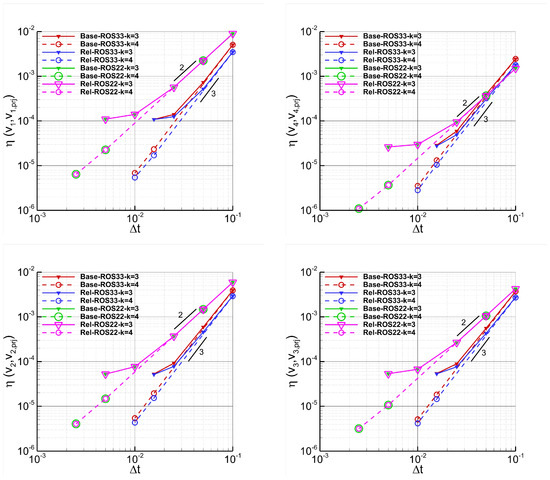
Figure 1.
Vortex–Time refinement study. Simulations performed with (Rel) and without (Base) relaxation, the EC flux, ROS22 and ROS33, dG approximations, and . The plots show the errors of the entropy variables , with , as a function of the time step sizes.
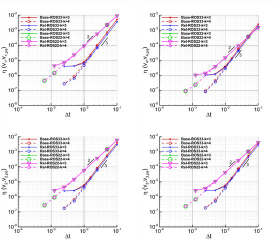
Figure 2.
Vortex–Time refinement study. Simulations performed with (Rel) and without (Base) relaxation, the ES flux, ROS22 and ROS33, dG approximations, and without over-integration. The plots show the errors of the entropy variables , with , as a function of the time step sizes.

Table 1.
Vortex–Lower error bound of the entropy variables , with . Simulations performed with ES and EC fluxes, dG approximation and a “small enough” time step size. Note that, since these values depend solely on spatial accuracy, the choice between the baseline and relaxation methods, as well as the use of ROS33 or ROS22, has no impact.
In Figure 3 the convergence of is shown for both EC and ES fluxes, where is the average value of the relaxation parameters over time. Since this is a simple transport problem, the values of computed at each time level are very close to their mean value, which is why was selected for representation. It can be observed that the theoretical convergence order of is satisfied for the ROS33 scheme, while for the ROS22 scheme the convergence order exceeds the theoretical value, approaching 2 for sufficiently small . Additionally, since for ROS22 is at least one order of magnitude smaller than for ROS33, ROS22 better preserves entropy. This could explain why for ROS22 the accuracy of the entropy variables is roughly the same with or without relaxation, whereas for ROS33 the relaxation technique leads to a slight improvement in accuracy compared to the baseline method, as shown in Figure 1 and Figure 2.
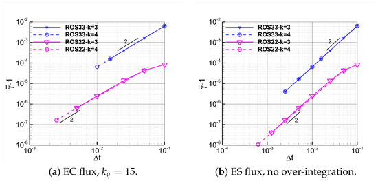
Figure 3.
Vortex–Time refinement study. Simulations performed with relaxation, ROS22 and ROS33 and dG approximations. The plots show the values as a function of the time step sizes.
Figure 4 and Figure 5 report the absolute values of for several variables computed with the EC and ES fluxes, respectively. It is worth noting that the sudden drops observed at some points are due to sign changes in the corresponding variables, and that the error of is shown without the absolute value, when the ES flux is used, to highlight that the entropy stability property is preserved. As expected, the plots show that the relaxation method achieves errors for equal to machine precision when the EC flux is used (see Figure 4), and that this error reaches the spatial accuracy limit even for large values of when the ES flux is used (see Figure 5). The ROS33 scheme achieves the expected order of convergence, while the ROS22 scheme has an order of convergence close to 3 for all variables, except for , for which a second-order convergence is observed. Furthermore, the results show that the ROS33 scheme equipped with the relaxation technique leads to a reduction of the error for with respect to the baseline method for both EC and ES fluxes, whereas no significant improvement is observed for the ROS22 scheme. For both time integration schemes and numerical fluxes, the relaxation method yields smaller errors for and compared to the baseline method, with the improvement being more pronounced for ROS33 than for ROS22, particularly for . Finally, it is worth noting that for both EC and ES fluxes, the ROS22 scheme, despite its lower order of accuracy relative to ROS33, produces smaller errors for and with the baseline method, and for when applied with either the baseline or relaxation methods.
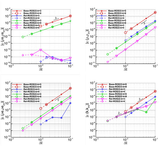
Figure 4.
Vortex–Time refinement study. Simulations performed with (Rel) and without (Base) relaxation, the EC flux, ROS22 and ROS33, dG approximations, and . The plots show the absolute values of the errors of several variables as a function of the time step sizes.
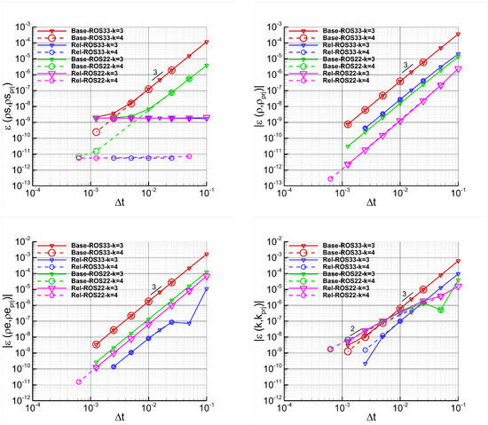
Figure 5.
Vortex–Time refinement study. Simulations performed with (Rel) and without (Base) relaxation, the ES flux, ROS22 and ROS33, dG approximations, and without over-integration. The plots show the absolute values of the errors of several variables as a function of the time step sizes. The entropy error is reported without absolute value.
4.2. The Kelvin-Helmholtz Instability
The Kelvin-Helmholtz instability (KHI) is a well-known phenomenon in fluid dynamics that occurs when there is a velocity shear between two fluid layers [33,34,35]. These simulations involve non-smooth flows featuring sharp discontinuities in velocity and density fields, alongside instabilities that drive the development of turbulence. The resulting turbulent flow is characterized by small structures that become progressively finer with increased spatial or temporal numerical resolution. This makes the numerical solution of the flow field highly sensitive to these parameters, as well as to small perturbations [36], which explains the significant variations observed in the results reported in the literature.
The initial flow field of this test-case is defined as follows:
where , and , a function designed to avoid flow field discontinuities.
The periodic computational domain is discretized using a uniform Cartesian grid, and the simulations are integrated in time up to . The simulations are performed using the ROS22 and ROS33 time integration schemes, different dG polynomial approximations, and several time step sizes. Furthermore, to evaluate the properties of the relaxation method under progressively more challenging conditions, the Atwood number has been varied in the range , where . Note that the Atwood number governs the driving force of the instability: small Atwood numbers indicate minimal density differences between the two fluids ( implies ), while higher Atwood numbers signify an increasing density imbalance ( implies ). As the Atwood number rises, the increasing density contrast amplifies shear at the interface, leading to stronger vortex formations, finer turbulent structures, and sharper velocity discontinuities, raising the risk of non-physical results, particularly in under-resolved simulations.
Table 2 and Table 3 present the simulation results obtained with the ES flux and without the use of over-integration technique, for and dG approximations, respectively. Overall, it is evident that, as the Atwood number increases, all discretizations, regardless of the dG approximations, time integration schemes or the use of the relaxation technique, exhibit reduced robustness. Furthermore, independently of the Atwood number, time integration or the use of the relaxation technique, by raising the dG approximation the method’s robustness decreases. Comparing the relaxed results with those obtained using the baseline method, it is evident that the relaxation technique does not lead to an overall improvement in robustness. This suggests that, in Kelvin–Helmholtz simulations without over-integration, its practical effect is limited, as the dominant source of instability arises from aliasing errors inherent in the spatial discretization. When over-integration is applied, as shown in Table 4 for dG approximations and , the robustness of both methods improves. These findings indicate that robustness is primarily governed by the accuracy of the quadrature rule, rather than by the relaxation technique.
Table 2.
KHI–Time refinement study performed with ROS33 and ROS22, dG approximation and different Atwood numbers. The simulations were carried out using the ES flux and without over-integration. The table reports the end time of the simulations. The blue color denotes the times that correspond to simulations which did not crash and ran to completion, the red color denotes simulations which did crash.
Table 3.
KHI–Time refinement study performed with ROS33 and ROS22, dG approximation and different Atwood numbers. The simulations were carried out using the ES flux and without over-integration. The table reports the end time of the simulations. The blue color denotes the times that correspond to simulations which did not crash and ran to completion, the red color denotes simulations which did crash.
Table 4.
KHI–Time refinement study performed with ROS33 and ROS22, dG approximation and different Atwood numbers. The simulations were carried out using the ES flux and over-integration with . The table reports the end time of the simulations. The blue color denotes the times that correspond to simulations which did not crash and ran to completion, the red color denotes simulations which did crash.
It is also worth noting that, even when both simulations, with and without relaxation, are run to completion, the resulting solutions exhibit noticeable differences. As an illustrative example, Figure 6 presents the density fields obtained without (Baseline) and with (Relaxed) the relaxation technique at . The simulations were performed with ROS33 with , a dG approximation and without over-integration. Both schemes capture the expected flow features of the instability, including the main vortices and the two mixing layers. However, clear differences arise in the two plots. In particular, the spatial position of the vortices clearly differs between the two formulations, a discrepancy consistent with the high sensitivity of compressible Kelvin–Helmholtz dynamics to small changes in numerical dissipation. In the baseline solution, the regions surrounding the vortices appear more irregular, while the relaxed solution exhibits a clearer separation between the vortical structures and the surrounding flow. Moreover, the density inside the vortex cores differs: the relaxed solution exhibits a stronger rarefaction, while in the baseline case the density drop is partially smeared out, indicating the presence of stronger numerical diffusion. In the central region between the two shear layers, the relaxed solution exhibits sharper gradients and thinner filaments, whereas the baseline solution is overly smoothed, suggesting the presence of stronger numerical diffusion.
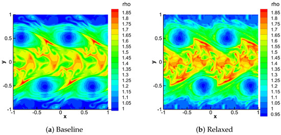
Figure 6.
KHI–Density fields at the final simulation time. Simulations performed at with the ES flux, ROS33 with , dG approximation, and without over-integration.
4.3. The Inviscid Taylor-Green Vortex
The relaxation method is here tested on the nearly incompressible inviscid Taylor-Green vortex (TGV). This is a very well-known test-case that has become a standard benchmark problem for high-order methods. In particular, the inviscid TGV is often used to assess the dissipative properties of the schemes, since at late enough simulation times, the flow will always be under-resolved. The interested reader can refer to [37,38] to better understand the fundamental mechanism involved in the laminar-turbulent transition of this flow.
The initial non-dimensional velocity components, pressure and density are given by:
where and . The free stream Mach number is equal to , which results in negligible compressibility effects.
The computational domain is a periodic cube with where , discretized with a uniform Cartesian grid composed by elements. The computations have been advanced in time up to .
Figure 7 and Figure 8 show, for the ROS33 and the ROS22 schemes, respectively, the evolution of the errors over time computed for , , and by using the EC flux and the over-integration technique. From the figures, it can be observed that the use of the relaxation technique not only ensures, as expected, a zero machine precision of , but also improves the conservation properties of all the other investigated quantities, especially when larger time step sizes are used and over longer time periods.
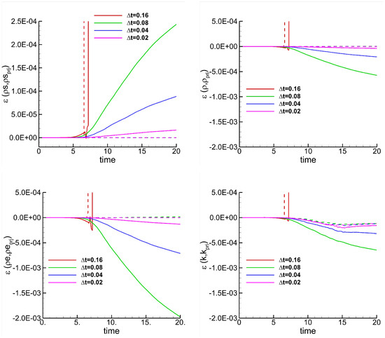
Figure 7.
TGV–Time refinement study. Simulations performed with (dashed line) and without (continuous line) relaxation, the EC flux, ROS33, dG approximation, and . The plots show the errors of several variables as a function of time for different time step sizes.
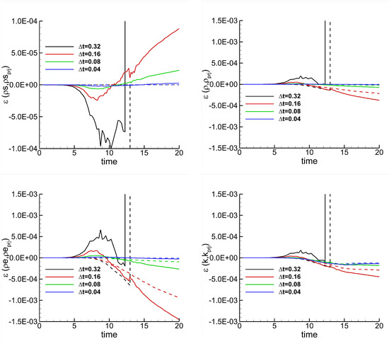
Figure 8.
TGV–Time refinement study. Simulations performed with (dashed line) and without (continuous line) relaxation, the EC flux, ROS22, dG approximation, and . The plots show the errors of several variables as a function of time for different time step sizes.
Table 5 presents the values of the errors of the same quantities reported in the figures at the final time . Overall, this table indicates that ROS22 exhibits greater robustness than ROS33, regardless of whether the relaxation technique is applied. Additionally, the values reported in the table demonstrate that, when the baseline scheme is used, ROS22 has better conservation properties with respect to ROS33. However, when the relaxation technique is used, the conservation properties of ROS33 scheme outperform those of ROS22.
Table 5.
TGV–Time refinement study. Simulations performed with and without relaxation (Baseline), the EC flux, ROS22 and ROS33, dG approximation, and . The table reports the errors of several variables at the end time of the simulations. The red cross symbol in the table indicates simulations that blow-up.
Figure 9 shows the temporal evolution of for two time steps obtained with ROS33 and ROS22. As illustrated in the plot and consistent with the behavior of the error shown in the previous figures, the ROS33 scheme, except for the very initial time steps, shows , indicating that the corresponding baseline scheme is dissipative at each time step, whereas for ROS22 fluctuates around 1, indicating a baseline scheme whose dissipative or anti-dissipative behavior varies over time. Furthermore, the correction introduced by the relaxation method is more pronounced for ROS33, which may explain why the relaxation technique has a greater impact on ROS33 than on ROS22, both in terms of solution accuracy and conservation properties.
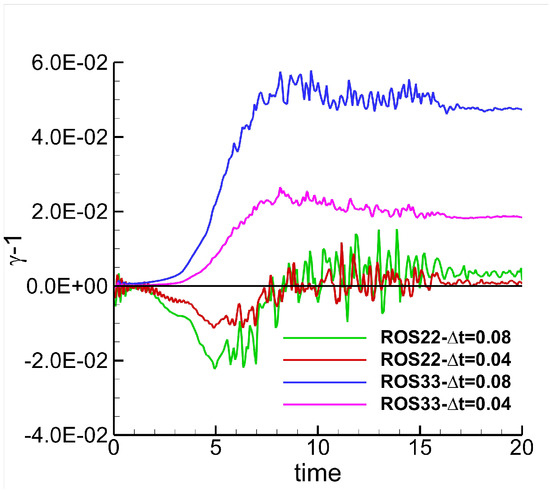
Figure 9.
TGV–Temporal evolution of . Simulations performed with EC flux, ROS22 and ROS33, dG approximation, and .
5. Conclusions
This work investigates the application of the relaxation technique to linearly implicit Rosenbrock-type Runge–Kutta schemes in the context of high-order entropy-conserving/stable discontinuous Galerkin (dG) discretizations of the compressible Euler equations. Originally developed to enforce entropy conservation or stability at the fully discrete level, the relaxation technique offers several advantages: it is straightforward to implement, requires no modifications to the time integration schemes, and preserves their theoretical convergence rates. The numerical results obtained for the isentropic convection problem indicate that the relaxation technique slightly improves the accuracy of the solution for ROS33. Another key finding is that, while entropy conservation or stability is guaranteed by construction, relaxed solutions also exhibit improved conservation of additional invariants. This improvement is evident not only in the inviscid isentropic vortex test case, but also in under-resolved flow regimes, such as those characterizing the Taylor–Green vortex. Regarding robustness, in the numerical experiments presented for the Taylor–Green vortex and the Kelvin-Helmholtz instability, the relaxation technique appears to have a limited impact, particularly when over-integration is not used. Nevertheless, in terms of accuracy, the Kelvin–Helmholtz tests show that the relaxation technique reduces numerical diffusion, producing clearer vortices and more detailed small-scale features.
Author Contributions
Conceptualization, A.N.; methodology, A.N.; software, E.C.; validation, A.N. and E.C.; writing—original draft preparation, A.N. and E.C.; writing—review and editing, A.N. All authors have read and agreed to the published version of the manuscript.
Funding
This research received no external funding.
Institutional Review Board Statement
Not applicable.
Informed Consent Statement
Not applicable.
Data Availability Statement
The data presented in this study are available from the corresponding author upon reasonable request.
Acknowledgments
We acknowledge CINECA for the availability of high-performance computing resources under the Italian Super-Computing Resource Allocation (ISCRA) initiative.
Conflicts of Interest
The authors declare no conflict of interest.
References
- Gear, C. Invariants and numerical methods for ODEs. Phys. Nonlinear Phenom. 1992, 60, 303–310. [Google Scholar] [CrossRef]
- Arakawa, A. Computational design for long-term numerical integration of the equations of fluid motion: Two-dimensional incompressible flow. Part I. J. Comput. Phys. 1966, 1, 119–143. [Google Scholar] [CrossRef]
- de Frutos, J.; Sanz-Serna, J.M. Accuracy and conservation properties in numerical integration: The case of the Korteweg-de Vries equation. Numer. Math. 1997, 75, 421–445. [Google Scholar] [CrossRef]
- Durán, A.; Sanz-Serna, J.M. The numerical integration of relative equilibrium solutions. Geometric theory. Nonlinearity 1998, 11, 1547. [Google Scholar] [CrossRef]
- Pazner, W.; Persson, P.O. Analysis and entropy stability of the line–based discontinuous Galerkin method. J. Sci. Comput. 2019, 80, 376–402. [Google Scholar] [CrossRef]
- Colombo, A.; Crivellini, A.; Nigro, A. On the entropy conserving/stable implicit DG discretization of the Euler equations in entropy variables. Comput. Fluids 2022, 232, 105198. [Google Scholar] [CrossRef]
- Hughes, T.J.; Franca, L.P.; Mallet, M. A new finite element formulation for computational fluid dynamics: I. Symmetric forms of the compressible Euler and Navier–Stokes equations and the second law of thermodynamics. Comput. Methods Appl. Mech. Eng. 1986, 54, 223–234. [Google Scholar] [CrossRef]
- Ismail, F.; Roe, P.L. Affordable, entropy–consistent Euler flux functions II: Entropy production at shocks. J. Comput. Phys. 2009, 228, 5410–5436. [Google Scholar] [CrossRef]
- Chandrashekar, P. Kinetic Energy Preserving and Entropy Stable Finite Volume Schemes for Compressible Euler and Navier-Stokes Equations. Commun. Comput. Phys. 2013, 14, 1252–1286. [Google Scholar] [CrossRef]
- Gottlieb, J.; Groth, C.P. Assessment of Riemann solvers for unsteady one–dimensional inviscid flows of perfect gases. J. Comput. Phys. 1988, 78, 437–458. [Google Scholar] [CrossRef]
- Colombo, A.; Crivellini, A.; Nigro, A. Entropy conserving implicit time integration in a Discontinuous Galerkin solver in entropy variables. J. Comput. Phys. 2023, 472, 111683. [Google Scholar] [CrossRef]
- Ketcheson, D.I. Relaxation Runge-Kutta methods: Conservation and stability for inner-product norms. SIAM J. Numer. Anal. 2019, 57, 2850–2870. [Google Scholar] [CrossRef]
- Ranocha, H.; Sayyari, M.; Dalcin, L.; Parsani, M.; Ketcheson, D.I. Relaxation Runge–Kutta Methods: Fully Discrete Explicit Entropy-Stable Schemes for the Compressible Euler and Navier–Stokes Equations. SIAM J. Sci. Comput. 2020, 42, A612–A638. [Google Scholar] [CrossRef]
- Ranocha, H.; Lóczi, L.; Ketcheson, D. General relaxation methods for initial-value problems with application to multistep schemes. Numer. Math. 2020, 146, 875–906. [Google Scholar] [CrossRef]
- Abgrall, R.; Le Mélédo, E.; Öffner, P.; Torlo, D. Relaxation Deferred Correction Methods and their Applications to Residual Distribution Schemes. SMAI J. Comput. Math. 2022, 8, 125–160. [Google Scholar] [CrossRef]
- Kang, S.; Constantinescu, E. Entropy–Preserving and Entropy–Stable Relaxation IMEX and Multirate Time–Stepping Methods. J. Sci. Comput. 2022, 93, 23. [Google Scholar] [CrossRef]
- Pareschi, L.; Russo, G. Implicit–Explicit Runge–Kutta Schemes and Applications to Hyperbolic Systems with Relaxation. J. Sci. Comput. 2005, 25, 129–155. [Google Scholar]
- Linders, V.; Ranocha, H.; Birken, P. Resolving entropy growth from iterative methods. BIT Numer. Math. 2023, 63, 45. [Google Scholar] [CrossRef]
- Ranocha, H.; Ketcheson, D. Relaxation Runge–Kutta Methods for Hamiltonian Problems. J. Sci. Comput. 2020, 84, 17. [Google Scholar] [CrossRef]
- Ranocha, H.; Dalcin, L.; Parsani, M. Fully discrete explicit locally entropy-stable schemes for the compressible Euler and Navier–Stokes equations. Comput. Math. Appl. 2020, 80, 1343–1359. [Google Scholar] [CrossRef]
- Biswas, A.; Ketcheson, D. Multiple-Relaxation Runge Kutta Methods for Conservative Dynamical Systems. J. Sci. Comput. 2023, 97, 4. [Google Scholar] [CrossRef]
- Bassi, F.; Botti, L.; Colombo, A.; Ghidoni, A.; Massa, F. Linearly implicit Rosenbrock-type Runge-Kutta schemes applied to the Discontinuous Galerkin solution of compressible and incompressible unsteady flows. Comput. Fluids 2015, 118, 305–320. [Google Scholar] [CrossRef]
- Chen, T.; Shu, C.W. Entropy stable high order discontinuous Galerkin methods with suitable quadrature rules for hyperbolic conservation laws. J. Comput. Phys. 2017, 345, 427–461. [Google Scholar] [CrossRef]
- Baker, A.J.; Iannelli, G.S. A stiffly-stable implicit Runge-Kutta algorithm for CFD applications. AIAA Paper 1988, 88, 416. [Google Scholar]
- Lang, J.; Verwer, J. ROS3P-An accurate third-order Rosenbrock solver designed for parabolic problems. BIT Numer. Math. 2001, 41, 731–738. [Google Scholar] [CrossRef]
- Hairer, E.; Wanner, G. Solving Ordinary Differential Equations II: Stiff and Differential-Algebraic Problems, 2nd ed.; Springer Series in Computational Mathematics; Springer: Berlin/Heidelberg, Germany, 1996; Volume 14. [Google Scholar]
- PETSc Web Page. Available online: https://petsc.org (accessed on 25 November 2025).
- Hairer, E.; Nørsett, S.P.; Wanner, G. Solving Ordinary Differential Equations I: Nonstiff Problems, 2nd Revised. ed.; Springer: Berlin/Heidelberg, Germany, 1993. [Google Scholar]
- Yee, H.C.; Sandham, N.D.; Djomehri, M.J. Low–dissipative high–order shock–capturing methods using characteristic–based filters. J. Comput. Phys. 1999, 150, 199–238. [Google Scholar] [CrossRef]
- Hu, C.; Shu, C.W. Weighted essentially non–oscillatory schemes on triangular meshes. J. Comput. Phys. 1999, 150, 97–127. [Google Scholar] [CrossRef]
- Nigro, A.; De Bartolo, C.; Bassi, F.; Ghidoni, A. Up to sixth-order accurate A-stable implicit schemes applied to the Discontinuous Galerkin discretized Navier–Stokes equations. J. Comput. Phys. 2014, 276, 136–162. [Google Scholar] [CrossRef]
- Spiegel, S.C.; Huynh, H.T.; DeBonis, J.R. A Survey of the Isentropic Euler Vortex Problem Using High-Order Methods. In Proceedings of the 22nd AIAA Computational Fluid Dynamics Conference, Dallas, TX, USA, 22–26 June 2015; pp. 1–21. [Google Scholar]
- Rueda-Ramírez, A.M.; Pazner, W.; Gassner, G.J. Subcell limiting strategies for Discontinuous Galerkin spectral element methods. Comput. Fluids 2022, 247, 105627. [Google Scholar] [CrossRef]
- Chan, J.; Ranocha, H.; Rueda-Ramírez, A.M.; Gassner, G.; Warburton, T. On the entropy projection and the robustness of high order entropy stable discontinuous Galerkin schemes for under–resolved flows. Front. Phys. 2022, 10, 898028. [Google Scholar] [CrossRef]
- Alberti, L.; Carnevali, E.; Colombo, A.; Crivellini, A. An entropy conserving/stable discontinuous Galerkin solver in entropy variables based on the direct enforcement of entropy balance. J. Comput. Phys. 2024, 508, 113007. [Google Scholar] [CrossRef]
- Schroeder, P.W.; John, V.; Lederer, P.L.; Lehrenfeld, C.; Lube, G.; Schöberl, J. On reference solutions and the sensitivity of the 2D Kelvin–Helmholtz instability problem. Comput. Math. Appl. 2019, 77, 1010–1028. [Google Scholar] [CrossRef]
- Brachet, M.E.; Meiron, D.; Orszag, S.; Nickel, B.; Morf, R.; Frisch, U. The Taylor-Green vortex and fully developed turbulence. J. Stat. Phys. 1984, 34, 1049–1063. [Google Scholar] [CrossRef]
- Shu, C.W.; Don, W.S.; Gottlieb, D.; Schilling, O.; Jameson, L. Numerical Convergence Study of Nearly Incompressible, Inviscid Taylor–Green Vortex Flow. J. Sci. Comput. 2005, 24, 1–27. [Google Scholar] [CrossRef]
Disclaimer/Publisher’s Note: The statements, opinions and data contained in all publications are solely those of the individual author(s) and contributor(s) and not of MDPI and/or the editor(s). MDPI and/or the editor(s) disclaim responsibility for any injury to people or property resulting from any ideas, methods, instructions or products referred to in the content. |
© 2025 by the authors. Licensee MDPI, Basel, Switzerland. This article is an open access article distributed under the terms and conditions of the Creative Commons Attribution (CC BY) license (https://creativecommons.org/licenses/by/4.0/).