
Mixed Recharge and Epikarst Role in a Complex Metamorphic Karst Aquifer: The Pollaccia System, Apuan Alps (Tuscany, Italy)


Abstract
:1. Introduction
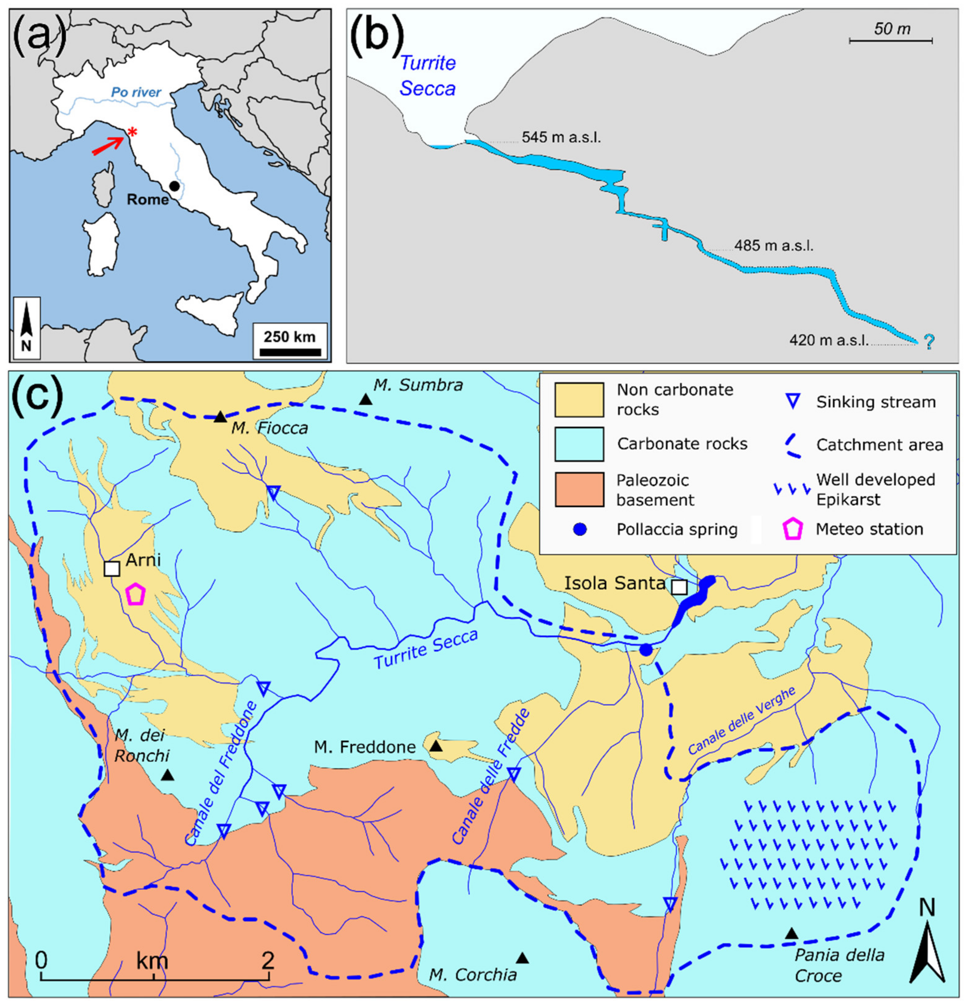
2. Study Area
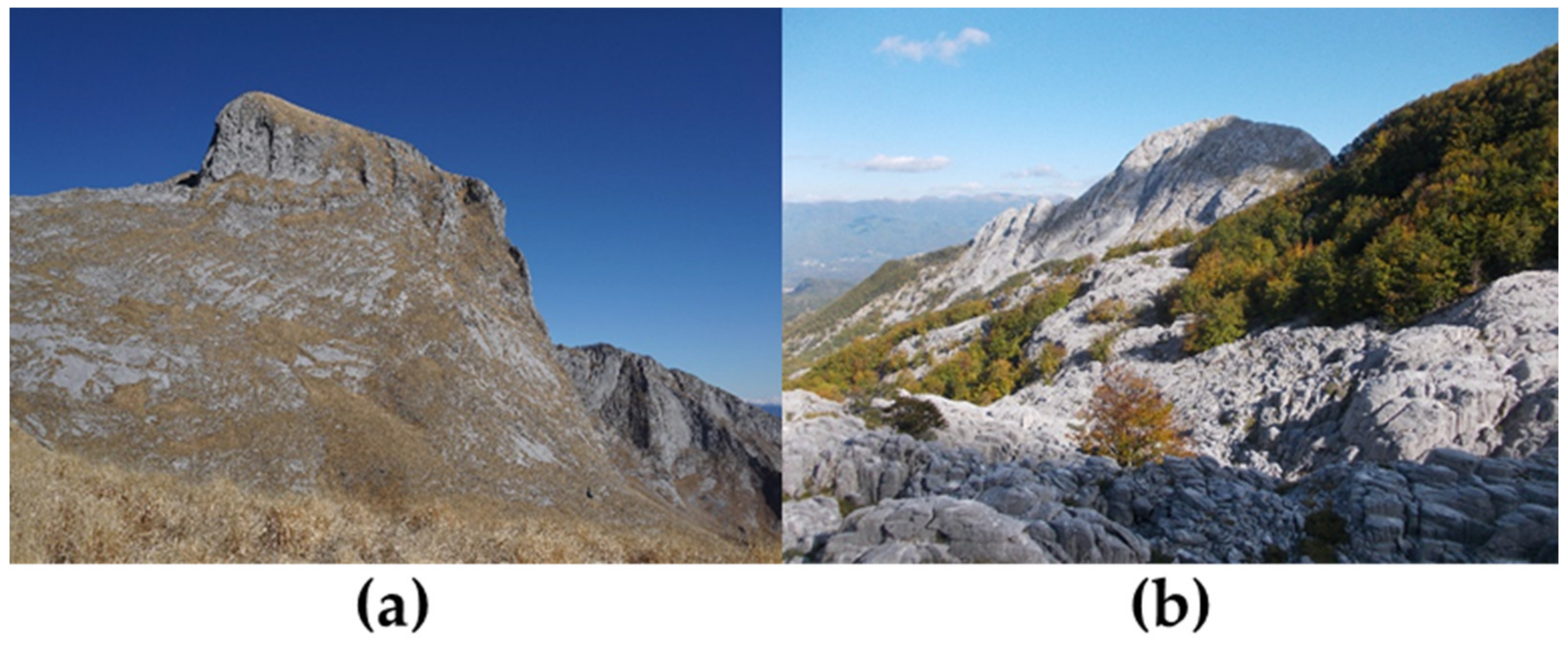
2.1. Geomorphological and Geological Setting
2.2. Hydrogeology
3. Methods
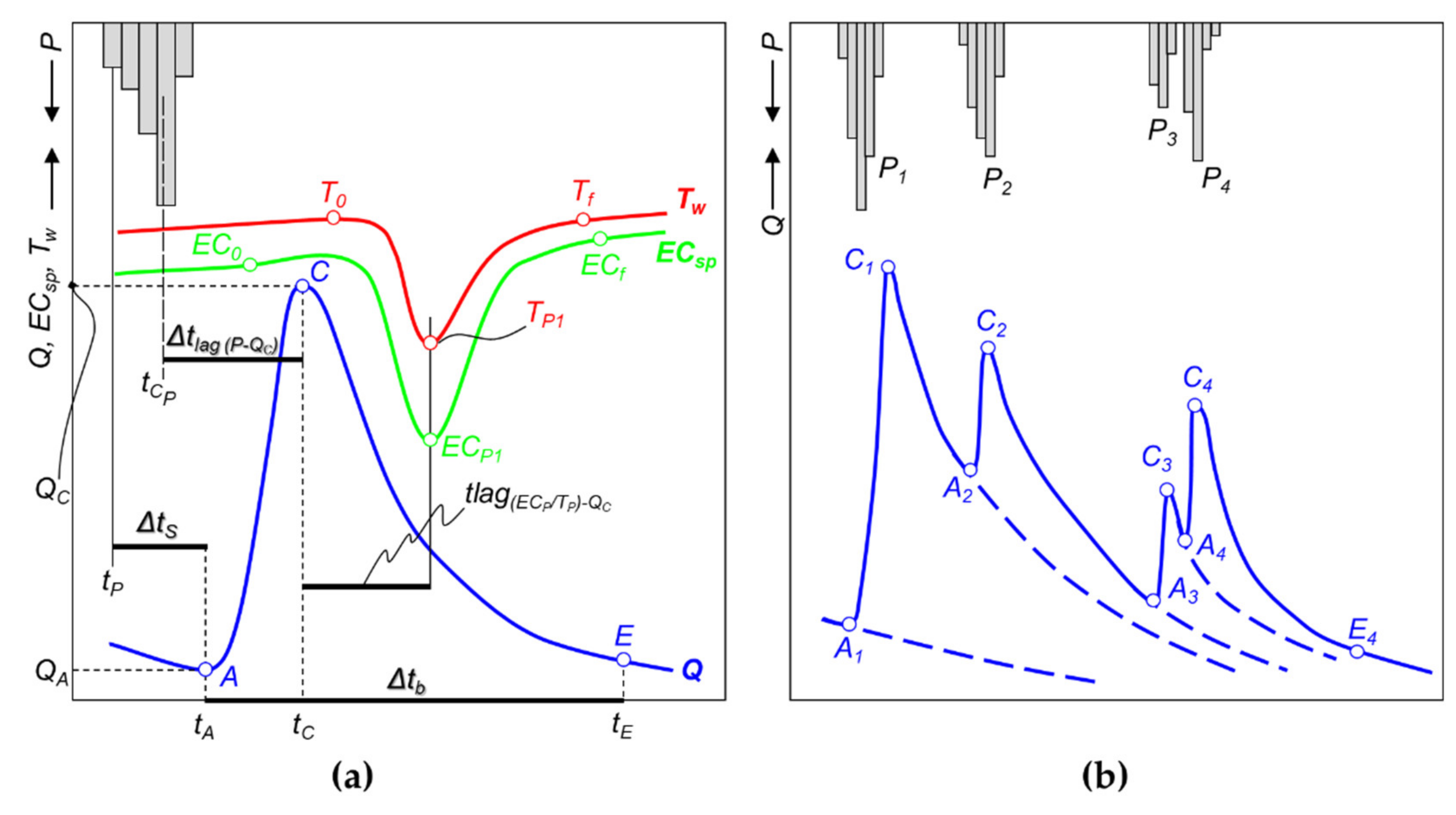
Storm Hydrographs and Lags Measurements
4. Results
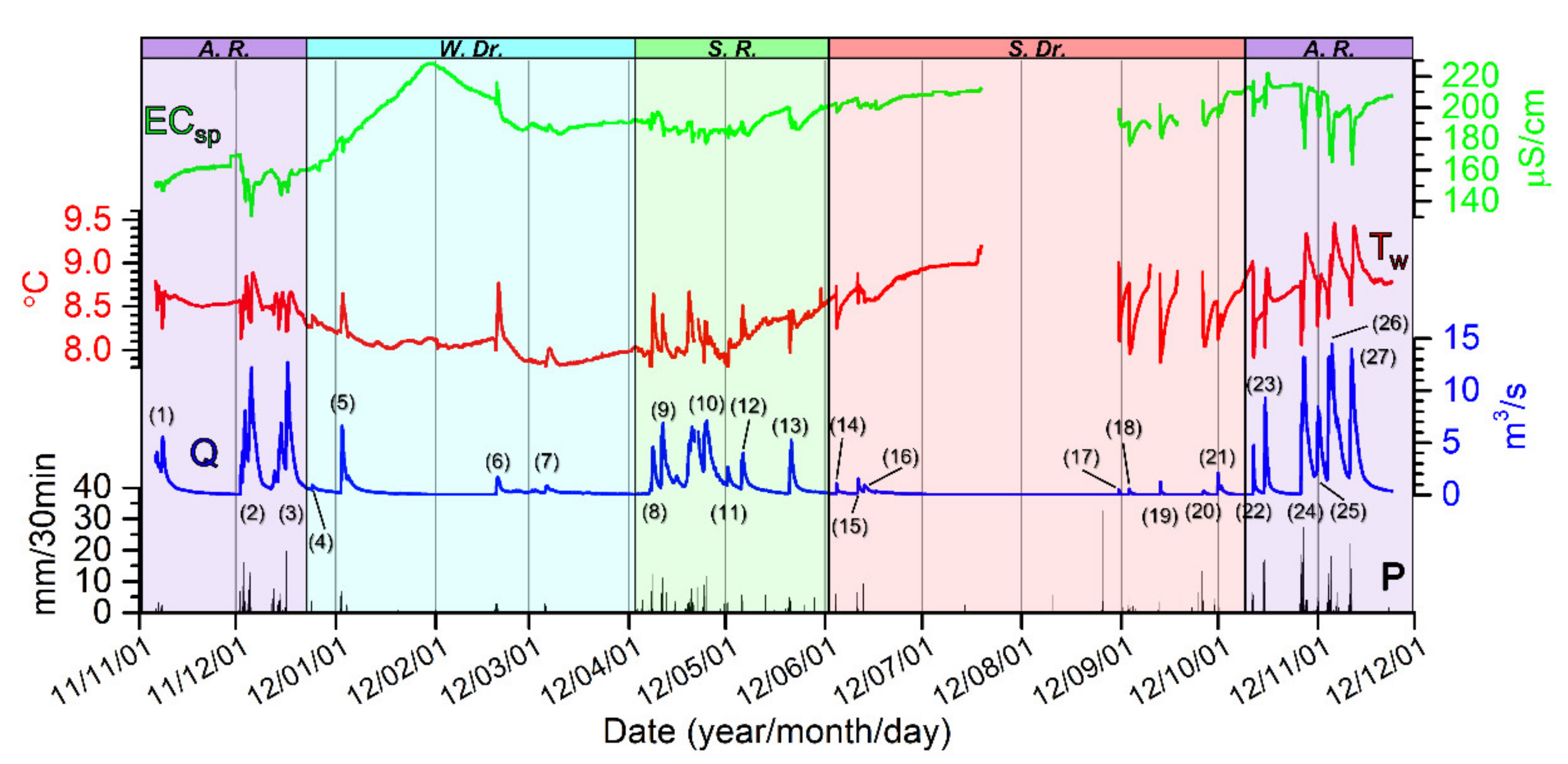
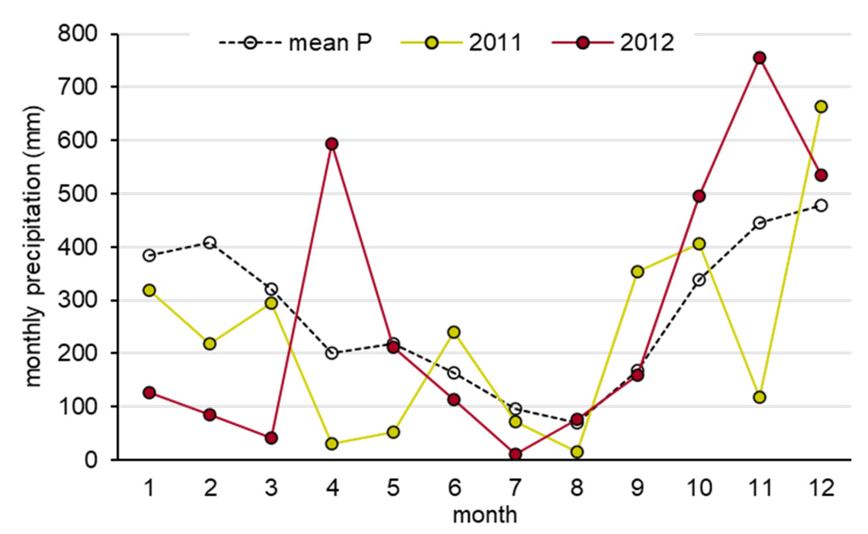
4.1. Hydrological Monitoring
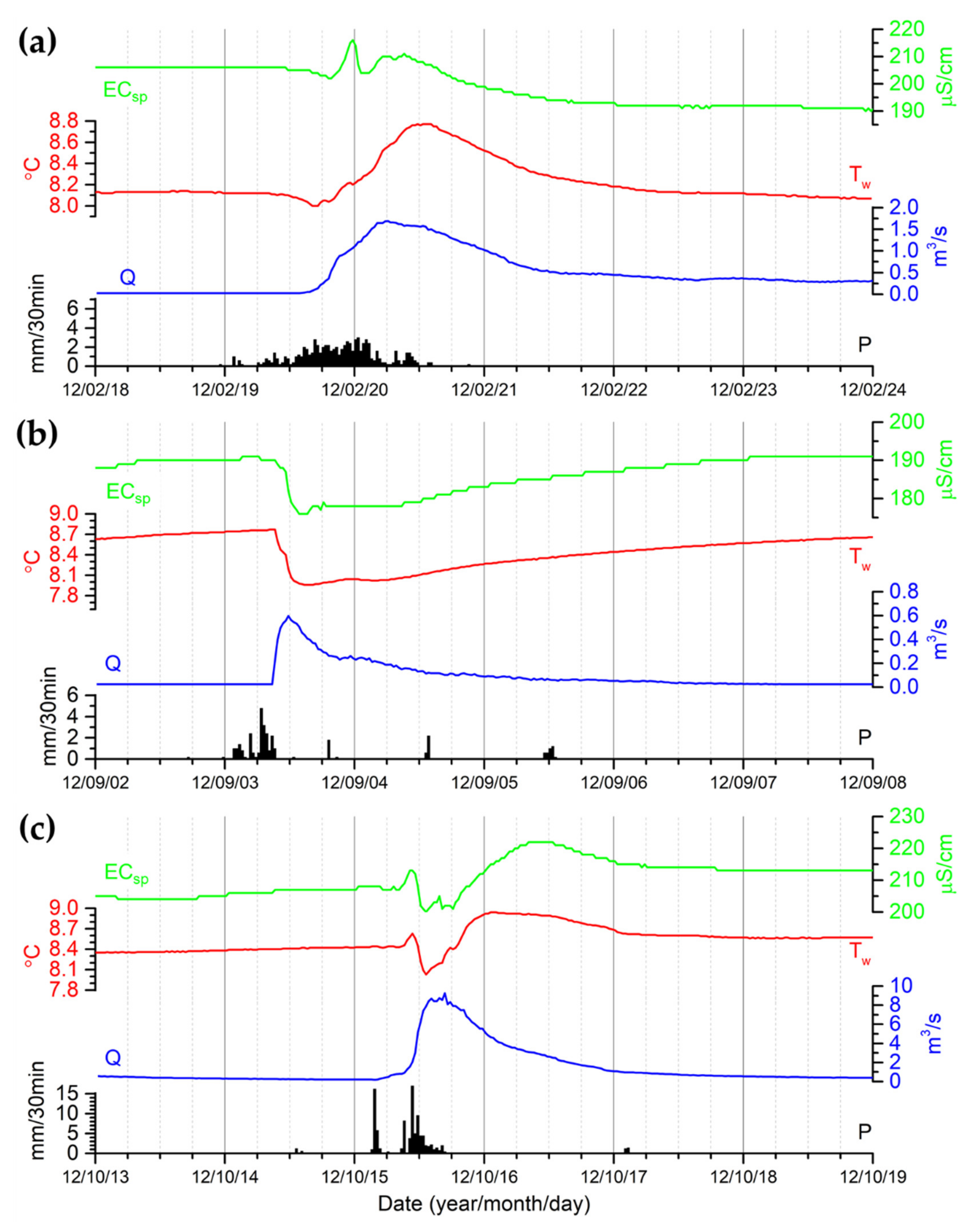
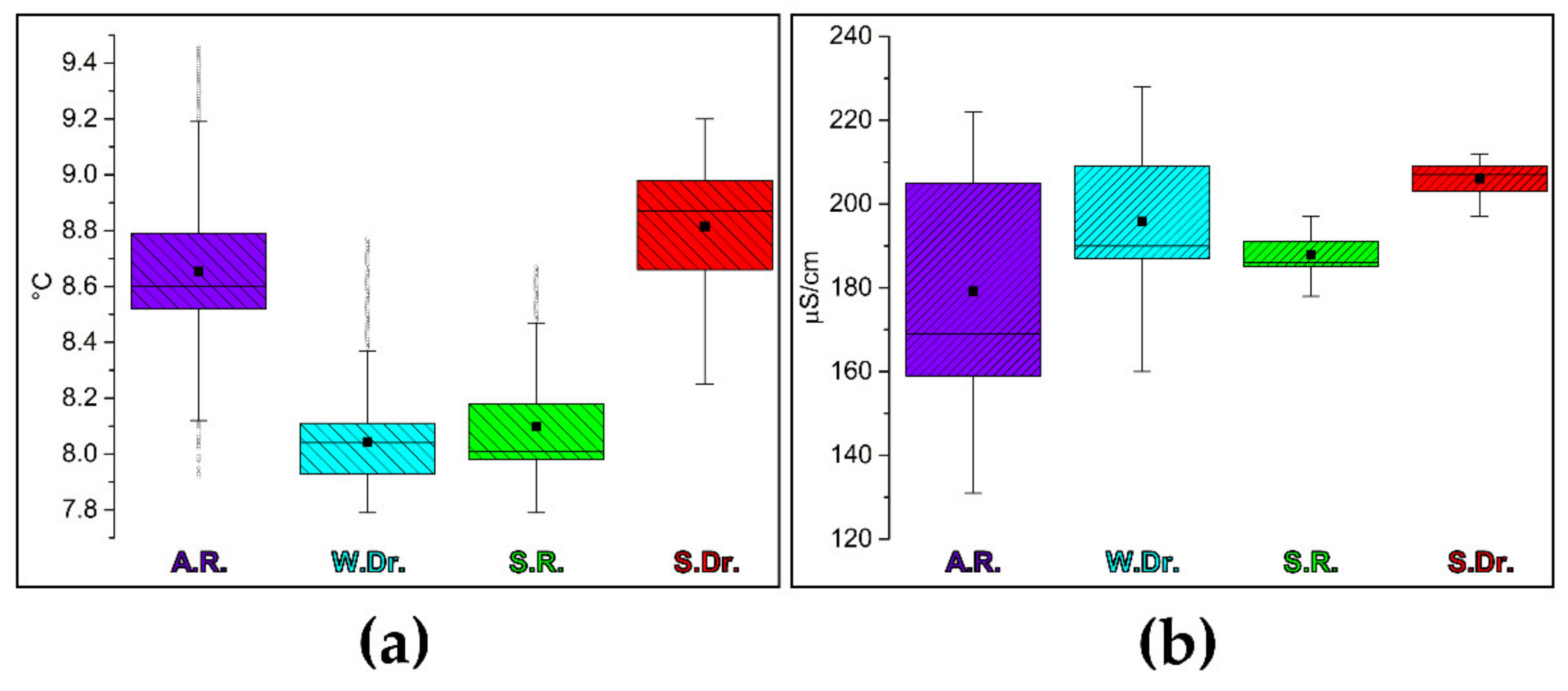
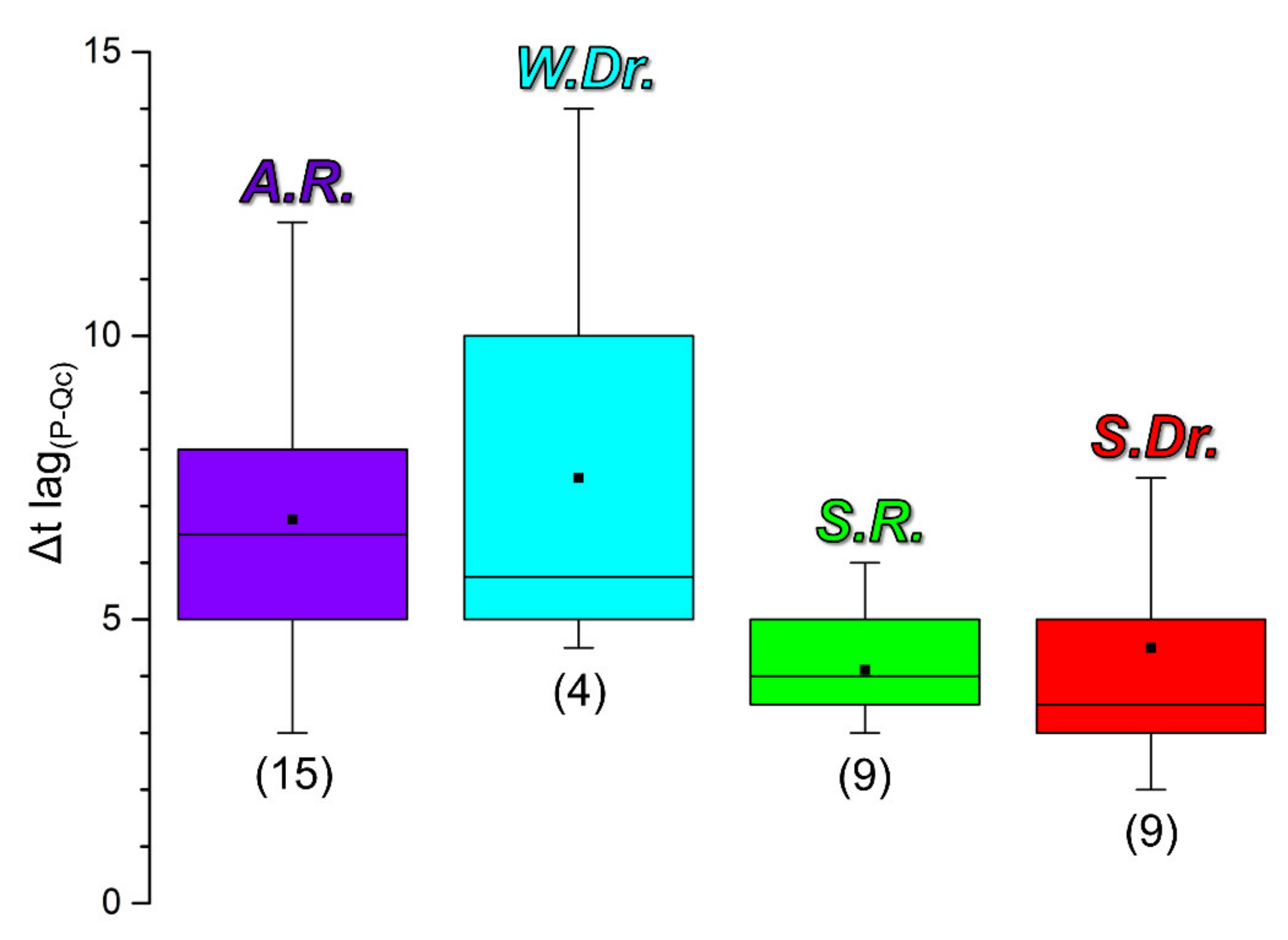
4.2. Storm HTC-Graph Analysis
5. Discussion
5.1. Spring Recharge/Discharge Hydrodynamics
5.2. Drought HTC-Graph Analysis
6. Conclusions
Supplementary Materials
Author Contributions
Funding
Data Availability Statement
Acknowledgments
Conflicts of Interest
References
- Ford, D.; Williams, P.D. Karst Hydrogeology and Geomorphology; John Wiley & Sons: Chichester, UK, 2007. [Google Scholar]
- Jukić, D.; Denić-Jukić, V. Groundwater balance estimation in karst by using a conceptual rainfall–runoff model. J. Hydrol. 2009, 373, 302–315. [Google Scholar] [CrossRef]
- Hartmann, A.; Goldscheider, N.; Wagener, T.; Lange, J.; Weiler, M. Karst water resources in a changing world: Review of hydrological modeling approaches. Rev. Geophys. 2014, 52, 218–242. [Google Scholar] [CrossRef]
- Bakalowicz, M. The epikarst, the skin of karst. In Epikarst, Special Publication, 9th ed.; Jones, W.K., Culver, D.C., Herman, J., Eds.; Karst Waters Institute: Leesburg, VA, USA, 2004; pp. 16–22. [Google Scholar]
- Williams, P.W. The role of the epikarst in karst and cave hydrogeology: A review. Int. J. Speleol. 2008, 37, 1–10. [Google Scholar] [CrossRef] [Green Version]
- Hartmann, A.; Baker, A. Modelling karst vadose zone hydrology and its relevance for paleoclimate reconstruction. Earth Sci. Rev. 2017, 172, 178–192. [Google Scholar] [CrossRef]
- Mangin, A. Karst Hydrogeology. In Groundwater Ecology; Gibert, J., Danielopol, D.L., Stanford, J.A., Eds.; Academic Press: New York, NY, USA, 1994; pp. 43–67. [Google Scholar]
- White, W.B. Karst hydrology: Recent developments and open questions. Engin. Geol. 2002, 65, 85–105. [Google Scholar] [CrossRef]
- Berglund, J.L. Karst Aquifer Recharge and Conduit Flow Dynamics from High-Resolution Monitoring and Transport Modeling in Central Pennsylvania Springs. Ph.D. Thesis, Temple University, Philadelphia, PA, USA, May 2019. [Google Scholar]
- Vigna, B.; Banzato, C. The hydrogeology of high-mountain carbonate areas: An example of some Alpine systems in southern Piedmont (Italy). Environ. Earth Sci. 2015, 74, 267–280. [Google Scholar] [CrossRef]
- Bonacci, O. Karst spring hydrographs as indicators of karst aquifers. Hydrol. Sci. J. 1993, 38, 51–62. [Google Scholar] [CrossRef]
- Goldscheider, N.; Drew, D. Methods in Karst Hydrogeology; IAH: International Contributions to Hydrogeology, 26; Taylor & Francis/Balkema: Leiden, The Netherlands, 2014. [Google Scholar]
- Desmarais, K.; Rojstaczer, S. Inferring source waters from measurements of carbonate spring response to storms. J. Hydrol. 2002, 260, 118–134. [Google Scholar] [CrossRef]
- Winston, W.E.; Criss, R.E. Dynamic hydrologic and geochemical response in a perennial karst spring. Water Resour. Res. 2004, 40, 05106. [Google Scholar] [CrossRef]
- Nannoni, A.; Vigna, B.; Fiorucci, A.; Antonellini, M.; De Waele, J. Effects of an extreme flood event on an alpine karst system. J. Hydrol. 2020, 590, 125493. [Google Scholar] [CrossRef]
- Liñán Baena, C.; Andreo, B.; Mudry, J.; Carrasco Cantos, F. Groundwater temperature and electrical conductivity as tools to characterize flow patterns in carbonate aquifers: The Sierra de las Nieves karst aquifer, southern Spain. Hydrogeol. J. 2009, 17, 843–853. [Google Scholar] [CrossRef]
- Sánchez, D.; Martín-Rodríguez, J.F.; Mudarra, M.; Andreo, B.; López-Rodríguez, M.; Navas, M.R. Time Lag Analysis of Natural Responses During Unitary Recharge Events to Assess the Functioning of Carbonate Aquifers in Sierra de Grazalema Natural Park (Southern Spain). In EuroKarst 2016, Neuchâtel. Advances in Karst Science; Renard, P., Bertrand, C., Eds.; Springer International Publishing: Cham, Switzerland, 2017; pp. 157–167. [Google Scholar] [CrossRef]
- Birk, S.; Liedl, R.; Sauter, M. Identification of localised recharge and conduit flow by combined analysis of hydraulic and physico-chemical spring responses (Urenbrunnen, SW-Germany). J. Hydrol. 2004, 286, 179–193. [Google Scholar] [CrossRef]
- Genthon, P.; Bataille, A.; Fromant, A.; D’Hulst, D.; Bourges, F. Temperature as a marker for karstic waters hydrodynamics. Inferences from 1 year recording at La Peyrére cave (Ariège, France). J. Hydrol. 2005, 311, 157–171. [Google Scholar] [CrossRef]
- Perrin, J.; Jeannin, P.Y.; Cornaton, F. The role of tributary mixing in chemical variations at a karst spring, Milandre, Switzerland. J. Hydrol. 2007, 332, 158–173. [Google Scholar] [CrossRef] [Green Version]
- Calligaris, C.; Galli, M.; Gemiti, F.; Piselli, S.; Tentor, M.; Zini, L.; Cucchi, F. Electrical conductivity as a tool to evaluate the various recharges of a Karst aquifer. Rend. Online Della Soc. Geol. Ital. 2019, 47, 13–17. [Google Scholar] [CrossRef] [Green Version]
- Chen, Z.; Hartmann, A.; Wagener, T.; Goldscheider, N. Dynamics of water fluxes and storages in an Alpine karst catchment under current and potential future climate conditions. Hydrol. Earth Sys. Sci. 2018, 22, 3807–3823. [Google Scholar] [CrossRef] [Green Version]
- Nerantzaki, S.D.; Nikolaidis, N.P. The response of three Mediterranean karst springs to drought and the impact of climate change. J. Hydrol. 2020, 591, 125296. [Google Scholar] [CrossRef]
- Fiorillo, F. Spring hydrographs as indicators of droughts in a karst environment. J. Hydrol. 2009, 373, 290–301. [Google Scholar] [CrossRef]
- Fiorillo, F.; Guadagno, F.M. Karst spring discharges analysis in relation to drought periods, using the SPI. Water Res. Managem. 2010, 24, 1867–1884. [Google Scholar] [CrossRef]
- Fiorillo, F.; Revellino, P.; Ventafridda, G. Karst aquifer draining during dry periods. J. Cave Karst Stud. 2012, 74, 148–156. [Google Scholar] [CrossRef]
- Petalas, C.P.; Moutsopoulos, K.N. Hydrogeologic behavior of a complex and mature karst aquifer system under drought condition. Environ. Processes 2019, 6, 643–671. [Google Scholar] [CrossRef]
- Lauritzen, S.E. Karst resources and their conservation in Norway. Nor. Geogr. Tidsskr. Nor. J. Geogr. 1991, 45, 119–142. [Google Scholar] [CrossRef]
- Lauritzen, S.E. Marble stripe karst of the scandinavian caledonides: An endmember in the contact karst spectrum. Acta Carsologica 2001, 30, 47–79. [Google Scholar]
- Filipponi, M.; Jeannin, P.Y.; Tacher, L. Evidence of inception horizons in karst conduit networks. Geomorphology 2009, 106, 86–99. [Google Scholar] [CrossRef]
- Andreo, B.; Carrasco, F.; De Galdeano, C.S. Types of carbonate aquifers according to the fracturation and the karstification in a southern Spanish area. Environ. Geol. 1997, 30, 163–173. [Google Scholar] [CrossRef]
- Despain, J.D.; Stock, G.M. Geomorphic history of Crystal Cave, Southern Sierra Nevada, California. J. Cave Karst Stud. 2005, 67, 92–102. [Google Scholar]
- Antonellini, M.; Nannoni, A.; Vigna, B.; De Waele, J. Structural control on karst water circulation and speleogenesis in a lithological contact zone: The Bossea cave system (Western Alps, Italy). Geomorphology 2019, 345, 106832. [Google Scholar] [CrossRef]
- Doveri, M.; Piccini, L.; Menichini, M. Hydrodynamic and geochemical features of metamorphic carbonate aquifers and implications for water management: The Apuan Alps (NW Tuscany-Italy) case study. In Karst Water Environment; Younos, T., Schreiber, M., Kosič Ficco, K., Eds.; Springer International Publishing: Cham, Switzerland, 2019; pp. 209–249. [Google Scholar]
- Piccini, L. Evolution of karst in the Alpi Apuane (Italy): Relationships with the morphotectonic history. Suppl. Geogr. Fis. E Din. Quat. III 1998, 4, 21–31. [Google Scholar]
- Kligfield, R.; Hunziker, J.; Dallmeyer, R.D.; Schamel, S. Dating of deformational phases using K-Ar and 40Ar/39Ar techniques: Results from the Northern Apennines. J. Struct. Geol. 1986, 8, 781–798. [Google Scholar] [CrossRef]
- Carmignani, L.; Kligfield, R. Crustal extension in the Northern Apennines: The transition from compression to ex-tension in the Alpi Apuane Core Complex. Tectonics 1990, 9, 1275–1303. [Google Scholar] [CrossRef]
- Conti, P.; Di Pisa, A.; Gattiglio, M.; Meccheri, M. Prealpine basement in the Alpi Apuane (Northern Apennines, Italy). In Pre-Mesozoic Geology in the Alps; Von Raumer, J.F., Neubauer, F., Eds.; Springer Verlag: Berlin/Heidelberg, Germany, 1993; pp. 609–621. [Google Scholar]
- Ottria, G.; Molli, G. Superimposed brittle structures in the late-orogenic extension of the Northern Apennine: Results from the Carrara area (Alpi Apuane, NW Tuscany). Terra Nova 2000, 12, 52–59. [Google Scholar] [CrossRef]
- Piccini, L. Acquiferi carbonatici e sorgenti carsiche delle Alpi Apuane. In Proceedings of the Le Risorse Idriche Sotterranee Delle Alpi Apuane: Conoscenze Attuali e Prospettive di Utilizzo, Forno di Massa, Italy, 22 June 2002; pp. 41–76. [Google Scholar]
- Piccini, L.; Giannini, E.; Malcapi, V.; Poggetti, E.; Steinberg, B. Monitoraggio idrodinamico di un sistema carsico: Risultati preliminari di un anno d’indagini alla sorgente Pollaccia (Alpi Apuane—Toscana). In Proceedings of the La Ricerca Carsologica in Italia, Fabrosa Soprana, Italy, 22–23 June 2013; pp. 147–154. [Google Scholar]
- USDA. NRCS. Chapter 3. Hydraulics. In National Engineering Handbook, Part 650, Engineering Field Handbook; USDA: Washington, DC, USA, 2001. [Google Scholar]
- Kresic, N.; Stevanovic, Z. Groundwater Hydrology of Springs: Engineering, Theory, Management and Sustainability; Butterworth-heinemann: Oxford, UK, 2009. [Google Scholar]
- Cholet, C.; Steinmann, M.; Charlier, J.B.; Denimal, S. Comparative study of the physicochemical response of two karst systems during contrasting flood events in the French Jura Mountains. In Hydrogeological and Environmental Investigations in Karst Systems. Environmental Earth Sciences; Andreo, B., Carrasco, F., Durán, J., Jiménez, P., LaMoreaux, J., Eds.; Springer: Berlin/Heidelberg, Germany, 2015; Volume 1, pp. 1–9. [Google Scholar] [CrossRef]
- Adji, T.N.; Bahtiar, I.Y. Rainfall–discharge relationship and karst flow components analysis for karst aquifer characterization in Petoyan Spring, Java, Indonesia. Environ. Earth Sci. 2016, 75, 1–10. [Google Scholar] [CrossRef]
- Piccini, L.; Nannoni, A.; Poggetti, E. Hydrodynamic of karst aquifers in metamorphic carbonate rocks: Results from spring monitoring in the Apuan Alps (Tuscany, Italy). Hydrogeol. J. 2022. under review. [Google Scholar]
- Piccini, L. Sui risultati della prova di colorazione all’abisso F. Orsoni—Vetricia (Apuane). Talp 1989, 1, 48–50. [Google Scholar]


| Parameter | Definition |
|---|---|
| Rising limb (A-C/concentration time (ΔtC) (h) | Storm hydrograph segment between the beginning of the flow increase (QA) and the the maximum discharge (QC) |
| QC-QA (m3/s) | Magnitude of the discharge increase |
| Falling limb (C-E)/falling time (Δtf) | Storm hydrograph segment between the maximum discharge (QC) and the end of the storm hydrograph (QE). |
| Storm hydrograph duration (Δtb) | Time elapsed between the beginning (A) and the end (E) of the storm hydrograph |
| ΔtP (h) | Time interval with no significant precipitation antecedent for each storm event |
| tP | Timing of the onset of precipitation |
| Starting time (Δts) (h) | Time elapsed between the onset of precipitation (tP) and the beginning of the rising limb (tA) |
| tCP | Timing of the centroid of precipitation |
| Pmax (mm/30 min) | Maximum precipitation intensity |
| Ptot (mm) | Total precipitation of a storm event |
| Prate (mm/h) | Precipitation rate |
| Lag time (Δt lag(P−Qc)) | Time elapsed between the centroid of the precipitation pulse (tP) and the maximum discharge (QC) |
| T0/EC0 | Temperature/specific conductivity value at the beginning of the oscillations caused by the storm event |
| T1/EC1 | Temperature/specific conductivity value of the first (positive or negative) peak caused by the storm event |
| Tf/ECf | Temperature/specific conductivity value at the end of the storm event |
| ΔTP1-0/ΔECP1-0 | Temperature/specific conductivity variation between T1/EC1 and T0/EC0 |
| ΔTf-0/ΔECf-0 | Temperature/specific conductivity variation between Tf/ECf and T0/EC0 |
| tlag(T/EC)-Qc | Time elapsed between the maximum discharge (QC) and TP1/ECP1 |
| Parameter | Statistical Index | Value |
|---|---|---|
| Qc–QA | Minimum | 0.28 |
| Maximum | 13.15 | |
| Mean | 3.96 | |
| Median | 2.78 | |
| Prate (mm/h) | Minimum | 0.00 |
| Maximum | 30.84 | |
| Mean | 6.48 | |
| Median | 4.84 | |
| ΔtP (h) | Minimum | 1.50 |
| Maximum | 577.00 | |
| Mean | 105.84 | |
| Median | 59.00 | |
| ΔtS (h) | Minimum | 0.00 |
| Maximum | 8.00 | |
| Mean | 3.18 | |
| Median | 2.50 | |
| Δt lag(P−Qc) (h) | Minimum | 2.00 |
| Maximum | 14.00 | |
| Mean | 5.65 | |
| Median | 5.00 | |
| Δt lag(Tpeak1-Qc) (h) | Minimum | −14.00 |
| Maximum | 4.50 | |
| Mean | −2.35 | |
| Median | −2.00 | |
| Δt lag(ECpeak1-Qc) (h) | Minimum | −6.50 |
| Maximum | 10.50 | |
| Mean | 1.62 | |
| Median | 1.50 |
| QC–QA | P Duration | Ptot | Prate | Pmax | ΔtP | ΔtS | ΔtC | Δt Lag(P−Qc) | |
|---|---|---|---|---|---|---|---|---|---|
| QC–QA | |||||||||
| P duration | 0.658 | ||||||||
| Ptot | 0.761 | 0.601 | |||||||
| Prate | 0.101 | −0.230 | 0.472 | ||||||
| Pmax | 0.653 | 0.256 | 0.695 | 0.619 | |||||
| ΔtP | −0.072 | 0.172 | −0.036 | −0.099 | −0.112 | ||||
| ΔtS | −0.147 | 0.341 | −0.068 | −0.392 | −0.383 | 0.181 | |||
| ΔtC | 0.615 | 0.918 | 0.618 | −0.135 | 0.332 | 0.156 | 0.163 | ||
| Δt lag(P−Qc) | 0.147 | 0.266 | 0.182 | −0.111 | −0.029 | 0.088 | 0.225 | 0.382 |
| Event | Hydrologic Phase | Peak Magnitude | T Fluctuation | EC Fluctuation | Hydrodynamic Response |
|---|---|---|---|---|---|
| 1 | AR | M-QC | − | − | d |
| 2 | AR | H-QC | − | − | d |
| 3 | AR | H-QC | − | − | d |
| 4 | WDr | L-QC | + | (+) | (p) |
| 5 | WDr | M-QC | +, − | (+), − | (p), d |
| 6 | WDr | L-QC | + | +, + | p, p |
| 7 | WDr | L-QC | (−), + | (−), + | (d), p |
| 8 | SR | M-QC | −, +, (−) | −, +, (−) | d, p, (d) |
| 9 | SR | M-QC | + | − | d |
| 10 | SR | M-QC | − | − | d |
| 11 | SR | L-QC | −, (+) | −, (+) | d, (p) |
| 12 | SR | L-QC | +, − | +, − | p, d |
| 13 | SR | L-QC | −, + | −, − | d, d |
| 14 | SDr | L-QC | (+), − | (+), − | (p), d |
| 15 | SDr | L-QC | (+), − | − | d |
| 16 | SDr | L-QC | (+) | (+) | (p) |
| 17 | SDr | L-QC | − | − | d |
| 18 | SDr | L-QC | − | − | d |
| 19 | SDr | L-QC | − | − | d |
| 20 | SDr | L-QC | (+), − | (+), − | (p), d |
| 21 | SDr | L-QC | −, + | −, + | d, p |
| 22 | AR | M-QC | − | (+), − | (p), d |
| 23 | AR | H-QC | (+), −, + | (+), −, + | (p), d, p |
| 24 | AR | H QC | −, + | − | d |
| 25 | AR | H-QC | − | − | d |
| 26 | AR | H QC | −, + | −, − | d, d |
| 27 | AR | H-QC | −, + | − | d |
Publisher’s Note: MDPI stays neutral with regard to jurisdictional claims in published maps and institutional affiliations. |
© 2022 by the authors. Licensee MDPI, Basel, Switzerland. This article is an open access article distributed under the terms and conditions of the Creative Commons Attribution (CC BY) license (https://creativecommons.org/licenses/by/4.0/).
Share and Cite
Nannoni, A.; Piccini, L. Mixed Recharge and Epikarst Role in a Complex Metamorphic Karst Aquifer: The Pollaccia System, Apuan Alps (Tuscany, Italy). Hydrology 2022, 9, 83. https://doi.org/10.3390/hydrology9050083
Nannoni A, Piccini L. Mixed Recharge and Epikarst Role in a Complex Metamorphic Karst Aquifer: The Pollaccia System, Apuan Alps (Tuscany, Italy). Hydrology. 2022; 9(5):83. https://doi.org/10.3390/hydrology9050083
Chicago/Turabian StyleNannoni, Alessia, and Leonardo Piccini. 2022. "Mixed Recharge and Epikarst Role in a Complex Metamorphic Karst Aquifer: The Pollaccia System, Apuan Alps (Tuscany, Italy)" Hydrology 9, no. 5: 83. https://doi.org/10.3390/hydrology9050083
APA StyleNannoni, A., & Piccini, L. (2022). Mixed Recharge and Epikarst Role in a Complex Metamorphic Karst Aquifer: The Pollaccia System, Apuan Alps (Tuscany, Italy). Hydrology, 9(5), 83. https://doi.org/10.3390/hydrology9050083