An Evaluation Matrix to Compare Computer Hydrological Models for Flood Predictions

Abstract

In order to predict and control the impacts of floods in torrents, it is important to verify the simulation accuracy of the most used hydrological models. The performance verification is particularly needed for applications in watersheds with peculiar climatic and geomorphological characteristics, such as the Mediterranean torrents. Moreover, in addition to the accuracy, other factors affect the choice of software by stakeholders (users, modellers, researchers, etc.). This study introduces a “performance matrix”, consisting of several evaluation parameters weighted by stakeholders’ opinions. The aim is to evaluate the accuracy of the flood prediction which is achieved by different models, as well as the pros and cons of software user experience. To this aim, the performances and requisites of four physical-based and conceptual models (HEC-HMS, SWMM, MIKE11 NAM and WEC-FLOOD) have been evaluated, by predicting floods in a midsized Mediterranean watershed (Mèsima torrent, Calabria, Southern Italy). In the case study, HEC-HMS and MIKE 11 NAM were the best computer models (with a weighted score of 4.45 and 4.43, respectively), thanks to their low complexity and computation effort, as well as good user interface and prediction accuracy. However, MIKE11 NAM is not free of charge. SWMM showed a lower prediction accuracy, which put the model in third place of the four models. The performance of WEC-FLOOD, although not being as good as for the other tested models, can be considered overall acceptable in comparison to the other well-consolidated models, considering that WEC-FLOOD is in the early stage of development. Overall, the proposal of the performance matrix for hydrological models may represent a first step in building a more complete evaluation framework of the hydrological and hydraulic commercial models, in order to give indications to allow potential users to make an optimal choice.

1. Introduction

Surface runoff, if not properly controlled, may cause several environmental impacts, such as flooding, soil erosion and transport of polluting compounds [1]. These impacts can be predicted by computer-based hydrological models on different temporal (from event-scale to decadal simulations) and spatial (from plot to continental) scales [2,3]. These models enable simulations of the effects of watershed processes and management activities in a cost-effective and time-efficient way [4]). For instance, the time and magnitude of floods can be predicted, often in real-time, allowing the authorities to forewarn the population [5]. Several watershed-scale models that vary in terms of complexity and data input requirement terms have been developed in recent decades [6]. For each model, application guidelines and reference manuals are available, but the developers’ indications sometimes cannot match the modellers’ needs [7].

Often, the choice of hydrological software among the computer models of different natures (e.g., empirical, physical-based and conceptual) and complexity can be a time-consuming and difficult task [8,9]. A modeller usually requires that a hydrological computer model is easily applicable, and has a low requirement of input data, especially when the model must be used in watersheds where geomorphological and hydrological input data are scarce (the so-called “data-poor environments”) [10,11]. Moreover, a model should offer a quick implementation procedure, a user-friendly software interface, a short computation time, a low purchase price (if it is not available for free), and, in addition, the high prediction accuracy of the modelled hydrological variables [7,12]. The latter is presumably the most important requisite that a potential user asks of a model, since the predictions must be as much accurate as possible and this requires field verification.

Very accurate hydrological predictions, such as runoff and erosion, are compulsory where the impacts of the watershed’s hydrology can be particularly serious, such as in torrents with small and steep watersheds under the semi-arid climate conditions of the Mediterranean Basin. In these watersheds, large runoff volumes are the hydrological response to frequent and intense rainstorms [13,14]. Many Mediterranean torrents are prone to high magnitude flash floods with high erosive power, often causing hydrogeological instability and disruption [15,16,17]. In these contexts (for instance in Southern Italy, Greece, Spain and Turkey), over the last 60–70 years the need to control and mitigate the hydrogeological risk has often forced local administrations to fund public works for soil conservation strategies [18,19], in order to avoid disruptive floods and debris flows. Despite this large body of work, the urban areas located downstream of these torrents are still subject to the flood risk with possible loss of human life and damages to civil infrastructures.

The capability of the most common hydrological models to predict runoff and erosion is not obvious in watersheds with peculiar climatic and geomorphological characteristics, such as the Mediterranean torrents. These watersheds are noticeably different from the environments, in which the hydrological models have been developed and validated [20,21], such as the United States. Therefore, in the Mediterranean torrents, targeted studies are required, which should test and verify the prediction accuracy of the most used computer models. Once validated, these models can be applied in several pieces of research and professional fields, and their use can simplify the analysis of watershed processes and the prediction of hydrological risks [12].

Although the literature proposes a very large number of studies evaluating the capacity of hydrological predictions of the most common computer models (e.g., [22,23]), there are far fewer evaluation tools to assess their practical applicability. There is the need for a framework aimed at identifying the most important “requisites”—e.g., input requirement, complexity, flexibility, computation effort—and evaluating the “performance” in terms of accuracy of hydrological predictions of computer models. Moreover, these requisites often depend on the experiences and skills of the modeller; thus, the framework should consider these subjective characteristics, but should provide a quantitative model evaluation regardless of the opinion of the individual user. In other words, this framework should give indications to a potential modeller, who wants to choose the most suitable software for hydrological applications. A case study for this evaluation in semi-arid watersheds is welcome, considering that the complex hydrological response of the Mediterranean torrents makes the choice of the most suitable hydrological model particularly difficult.

To satisfy this need, this study proposes a “model evaluation matrix” that compares the requisites and performances of hydrological computer models. The matrix consists of an ensemble of synthetic evaluation parameters, weighted by the interviews of 10 stakeholders (scholars, freelancers and public administration managers), which measure the requisite and flood prediction capability of the models, to provide a score. Four hydrological computer models (HEC-HMS, SWMM, MIKE11 NAM and WEC-FLOOD) have been compared using the developed evaluation matrix; specifically, the models have been calibrated and validated in a midsized Mediterranean watershed (Mèsima torrent, Calabria, Southern Italy) by using a database of 1.5-year observations of water discharge recorded at the torrent outlet.

The paper develops as follows: after a theoretical analysis of the proposed evaluation matrix of models (Section 2), the models to be tested are presented in Section 3.1. Then, the hydrologic and morphological characteristics of the watershed are presented (Section 3.2). Section 3.3 shows the calibration/validation procedures for each model. In Section 4, the results of the study are presented and discussed, with particular attention to both the model accuracy in predicting the water discharge at the watershed outlet and the evaluation matrix. Finally, in Section 5 the potential use of each model is suggested.

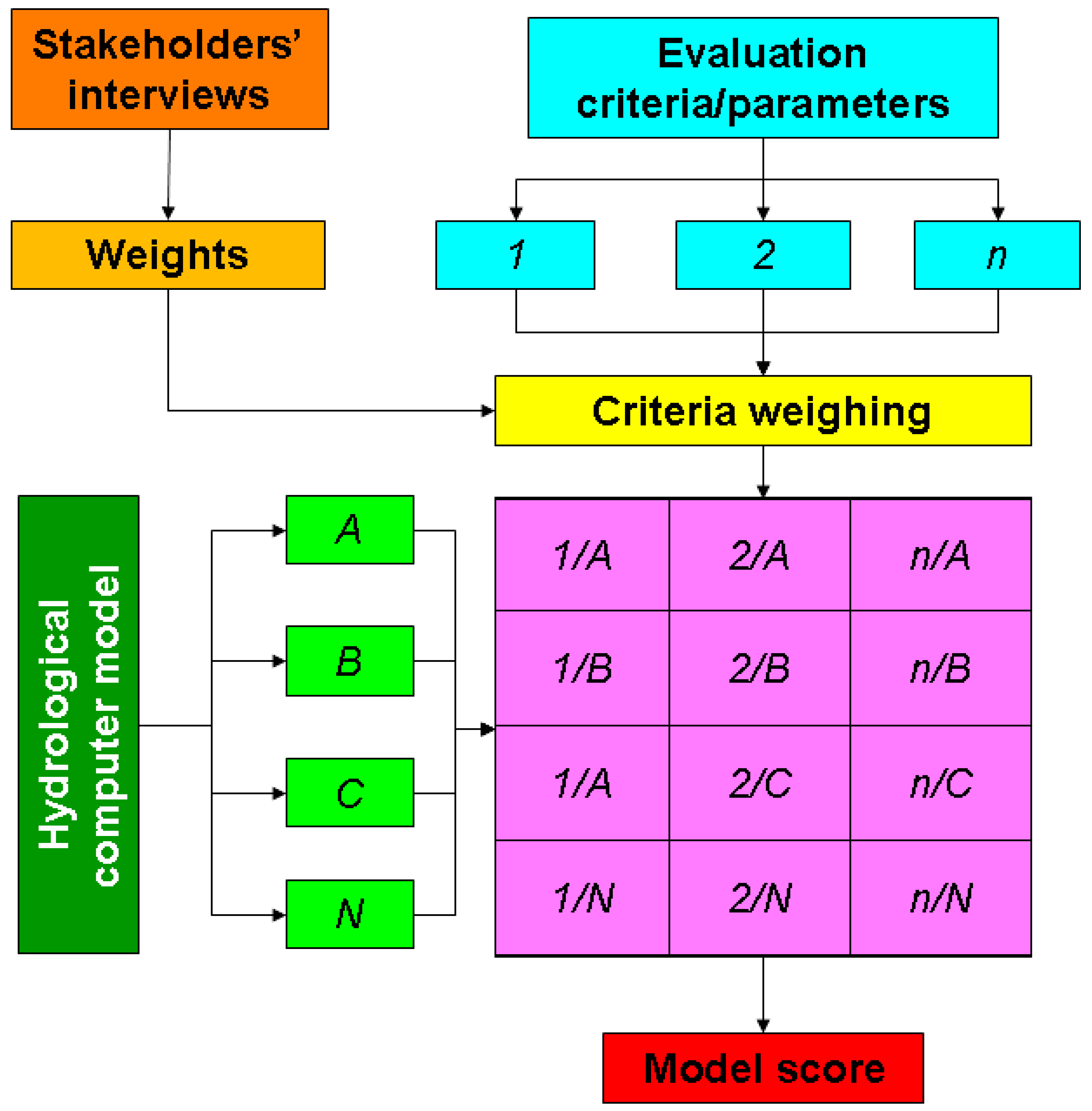
2. The Evaluation Matrix of Models

2.1. Description of the Matrix

The prediction accuracy is not the only requisite that a user asks a model, because other characteristics influence the choice of software for practical use. Moreover, most of the model characteristics depend on the stakeholders’ needs and opinions. This study introduces a “performance matrix”, consisting of several evaluation parameters weighted by stakeholders’ opinions. We propose an evaluation framework of computer hydrological models based on a matrix, consisting of 10 “criteria” Figure 1.

• Input requirement;
• Availability of input data;
• Complexity;
• User interface;
• Prediction accuracy;
• Range of time and space scales;
• Flexibility;
• Computation effort;
• Commercial cost;
• Compatibility with other software

The “input requirement” is the number of parameters needed by the algorithms to calculate the water discharge. The related scores of the models are calculated as the ratio between the minimum number of parameters required by each model to run and the highest number of parameters. The model performance related to this evaluation criterion can be assumed as the difference between one and this ratio.

The “availability of input data” is linked to the number of input parameters that can be collected from literature data and user manuals without making field measurements.

The “complexity” is how complicated it will be for the user to parameterise the watershed (in other words, it is a measure of the effort required to the modeller to input the watershed and climate data in the software for simulations); this performance could be measured using the time required by the user to be able to run the model.

The “user interface” is the character of user-friendliness of the software, which would be minimum for a simple TUI (Text-based User Interface) interface and optimal for software with a Graphical User Interface (GUI).

The “prediction accuracy” is the reliability of the simulations, evaluated through the statistics and indexes adopted in this study. In this regard, the ability of the model to reproduce the peak flow (the maximum of the hydrograph) or the total runoff volume (its area) or both accurately should be distinguished. In this study, using the statistics and indexes described in Section 2.2 and Table 3, the mean value of the percentage differences between the observed and predicted peak flows and runoff volumes were considered for each model. For this criterion, the model performance was evaluated as the difference between one and the ratio mean/maximum percentage difference.

The “range of time and space scales” relates to the model’s ability to take into account the temporal and spatial variability of the meteorological input and the physical conditions of the watershed. Indeed, in this sense, distributed and continuous models perform better than lumped and event-based models. The “flexibility” is the possibility, offered by the software, to predict a large number of environmental variables in addition to the water discharge (for instance, erosion, water quality and flood maps).

The “computation effort” is the time it takes to perform a complete run. The “cost” is the software licence fee which is zero for freeware software. Finally, the “compatibility with other software” is the possibility to interface the input or output of the model with other software, such as GIS tools, which is evaluated in terms of the number of formats which can be used for the input and output parameters.

Parameters 2, 3, 4, 6, 7 and 10 can assume only categorical values (the opinions of the user), while Parameters 1, 5, 8 and 9 are based on quantitative parameters (the number of input data, the time needed for simulation and the software price, respectively).

Based on these parameters, a 10 × 4 “performance” matrix (10 rows, one for each parameter, and four columns, one for each model) was built.

The seven categorical parameters, based on the user’s opinion, were evaluated, asking the user to give a score (between zero and five) for each software and parameter. These scores have been subsequently standardised between zero and one.

Since each parameter can be subjective, a set of weights were applied, to process the performance matrix. To this aim, 10 users coming from three different work categories (three researchers, three freelancers, and four public administration officials), were asked to give an opinion through a score (of importance ranging from a minimum of zero to a maximum of five) for each model’s performance and requisite. More specifically, two (full and associate) professors and one lecturer were interviewed among the researchers; one agronomist, one forest doctor and one hydraulic engineer were considered among the freelancers; finally, the public administration officials were four technicians working in two environmental agencies (two persons) and two Water User Associations (two other persons).

These scores were also standardised between zero and one and averaged, to calculate the weight of each of the 10 parameters. Overall, the perfect software should have a total performance equal to ten, while the worst software should have a total weighted score equal to zero.

2.2. Evaluation of the Prediction Accuracy

For each of the rainfall–runoff events, the water discharge was simulated at the torrent outlet using the four computer models. The simulations were analysed for “goodness-of-fit” with the corresponding observations. First, the observed and simulated values of the discharge were visually compared in scatter plots. A series of wide used parameters in the hydrological literature (e.g., [23,24,25,26,27,28,29]) was chosen to evaluate

• The main statistics (i.e., the maximum, minimum, mean and standard deviation of both the observed and simulated values);
• A set of summary and difference measures, such as the coefficient of determination (R²), coefficient of efficiency (E, [27]) and its modified form (E*, [24]), and Root Mean Square Error (RMSE). In particular, E is more sensitive to extreme values, while E* is better suited to significant over- or underprediction as it reduces the effect of squared terms. The related equations are reported in the works of [28,29,30].

The ranges of these indexes are:

• 0 < R² < 1, where values over 0.5 are acceptable [30,31];
• −∞ < E < 1 and −∞ < E* < 1. The model accuracy is “good” if E and E* ≥ 0.75, “satisfactory” if 0.36 ≤ E and E* ≤ 0.75 and “unsatisfactory” if E and E* ≤ 0.36 [30];
• 0 < RMSE < +∞, which measures the standard deviation between observations and predictions, should be as close as possible to zero [32]; RMSE is considered good if its predicted value is lower than 0.5 of the observed standard deviation [33].
• −∞ < CRM < +∞ is the Coefficient of Residual Mass and measures the tendency of the model to overestimate or underestimate the observations. Positive or negative values for CRM indicate model underestimation or overestimation, respectively.

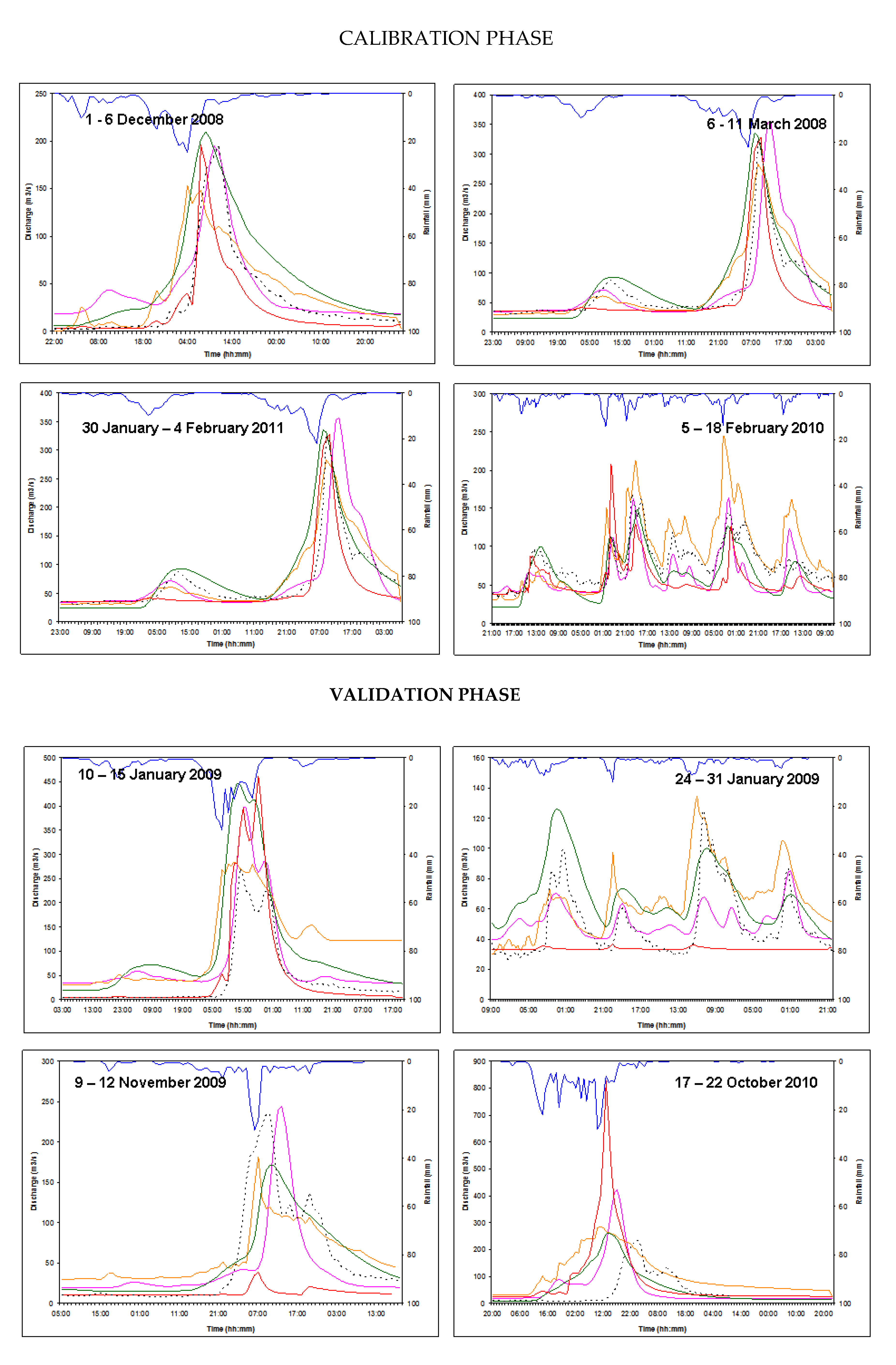
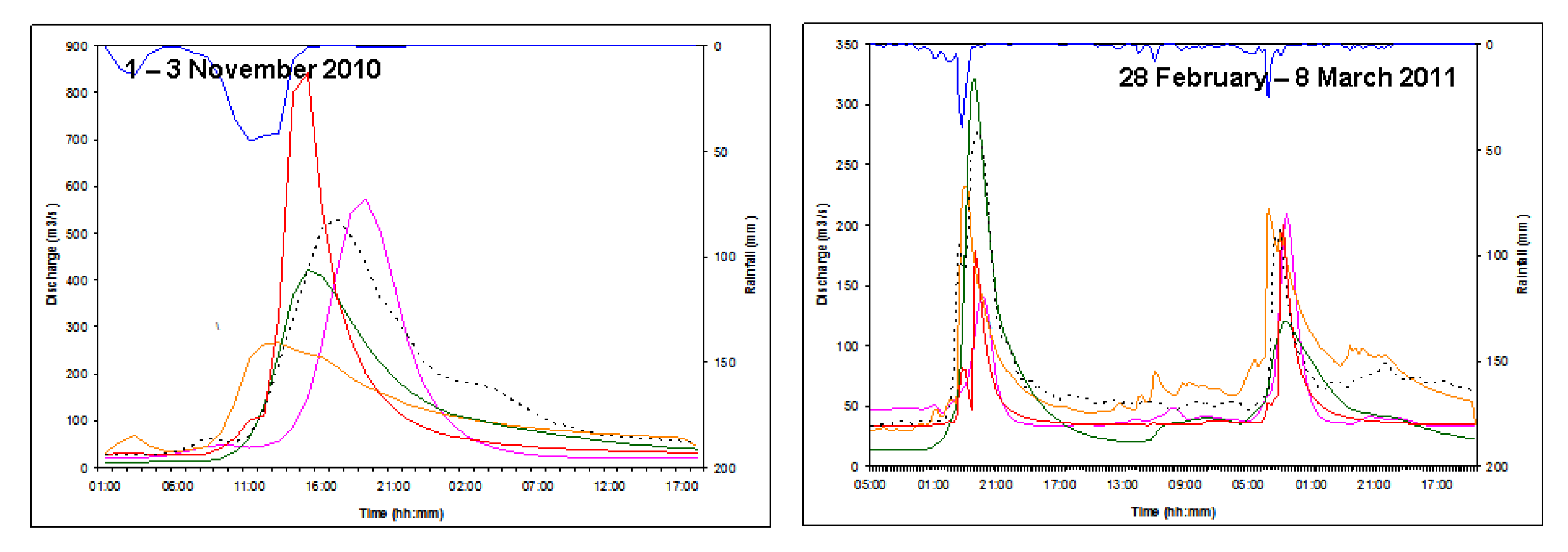
3. Case Study

3.1. The Hydrological Computer Models under Evaluation

Four computer hydrological models were chosen to test the evaluation matrix:

• HEC-HMS (Hydrologic Engineering Center—Hydrologic Modelling System, developed by the “US Army Corps of Engineers” [34]);
• SWMM (Storm Water Management Model, developed by the Environmental Protection Agency of USA [35]);
• MIKE11 NAM (Nedbør-Afstrømnings-Model, developed at the Institute of Hydrodynamics and Hydraulic Engineering at the Technical University of Denscore [36]);
• WEC-FLOOD (developed at the University of Palermo, Italy [37,38,39,40,41]).

In more detail, HEC-HMS is a lumped, event-based and conceptual hydrological model, which simulates the rainfall–runoff process and forecast streamflow in both large river basins and small urban or natural watersheds [42,43]. The model structure consists of four “components” [44,45]: (i) a basin model, which estimates hydrological losses and simulates the rainfall–runoff transformation; (ii) a meteorological model; (iii) a control specification subroutine, specifying the time step, the inception and the simulation period; and (iv) an input data subroutine, to provide the observed hydrological variables to the model. HEC-HMS uses separate methods to represent each component of the runoff process, including methods that compute runoff volume, direct runoff and baseflow. Runoff volume is calculated by the rainfall–runoff transformation method, based on the infiltration of pervious areas; a baseflow method is applied both at the start of a simulation of a storm event and later in the event, as the delayed subsurface flow reaches the watershed channels [42].

MIKE11 NAM is a conceptual, continuous and lumped rainfall–runoff model, which is included in the MIKE 11 module. By this model, water flows and sediment transport in rivers, irrigation systems, channels and other water bodies can be simulated at the watershed scale [46]; the model is also used to predict floods. MIKE11 NAM continuously accounts for the water content in three mutually interrelated storages that represent overland flow, interflow and base flow [47]. Each subcatchment is treated as one unit with averaged spatial parameters and variables. Nine parameters, of empirical and conceptual nature, represent a surface zone, root zone, and groundwater storage; the upper and lower boundary is defined by default values, which can be setup using both manual and autocalibration methods included in the software, depending on the watershed characteristics [48], to adjust the parameters [49,50].

SWMM is a distributed, continuous and physical-based rainfall–runoff model, which consists of several different components named “blocks”. As regards the runoff predictions, the “Runoff” block simulates hydrographs using the weather data and the physical and hydrologic characteristics of the watershed as input [51]. Surface runoff is generated in each subwatershed, in which the watershed is discretised. An individual subwatershed is modelled as a nonlinear reservoir with rainfall as input, when the water depth is greater than the maximum depression storage of both pervious and impervious areas. Infiltration in pervious areas is estimated using SCS-Curve Number (CN), Horton’s or Green–Ampt’s methods. The “Transport” block, simulating flow transport by steady wave routing, kinematic wave routing and dynamic wave routing, uses the output from the Runoff block as input and models the open channels and sewer system as a series of geometrical hydraulic elements, based on De Saint-Venant’s equations under 1D form (a simplification of the shallow water equations with a 2D form) [51,52].

WEC-FLOOD is a distributed, continuous and physical-based hydraulic model, which is suitable to simulate the rainfall–runoff process and flooding events affecting urban areas [37,38]. One-dimensional (1D) spatial discretisation of the main rivers is coupled with a 2D discretisation of flood-affected areas, but neither boundary condition must be solved at the transition between the 1D–2D domains, nor additional variables must be introduced in the model [38]. WEC-FLOOD simulations are carried out through numerical integration of the diffusive approximation of Saint-Venant’s partial differential equations, using the MArching in Space and Time approach [39,40,41]. The governing equations are discretised using an unstructured hybrid mesh with triangular and quadrilateral elements. One-dimensional (1D) channels are discretised using quadrilateral elements, with one couple of opposite edges overlapping the trace of two river sections and the other couple connecting their ends. The trace of each river section is extended up to the minimum topographic elevation where 1D flow conditions are expected. The 2D computational domain is given by the all area of the catchment basin and the flood plains and is discretised with triangular elements satisfying the Generalised Delaunay conditions [39]. WEC-FLOOD computes, at each time step, the net rain falling in each computational cell of the 2D domain, given the total rain and the water content, which is updated for the next time step. To this end the model can incorporate several possible hydrological transformations, to be selected according also to the available soil data. The outputs of the model are the main flow characteristics at each node of the computational domain, such as the velocity and the flow direction.

As a summary, in

Table 1. Main characteristics of the software applied to the Mesima torrent (Calabria, Southern Italy).

Model Characteristic	Software
	HEC-HMS	MIKE11 NAM	SWMM	WEC-FLOOD
Spatial scale (distributed/lumped)	Lumped		Distributed
Time scale (continuous/event)	Event	Continuous
Type of hydrological process modelling (empiric/conceptual/physical-based)	Conceptual		Physical-based
Approach to the hydrological processes (deterministic/stochastic)	Deterministic

, a classification of the four types of software, according to their main characteristics and following the model categories suggested by [3] is reported. In more detail, with regards the spatial scale, “distributed” models reflect the spatial variability of processes and outputs in the catchment of analysis [7], while “lumped” models simulate the hydrological processes in a watershed with mean geomorphological and climatic characteristics. Concerning the temporal resolution, while the “event-based” models are developed to assess the response of the modelled area to single storm events, the “continuous” models simulate this response based on a continuous balance of the water content of soil and this allows predicting changes in vegetation or land management over time. The distinction of model structure (empirical vs. conceptual vs. physical-based) is not sharp and therefore can be somewhat subjective [3]. Empirical models are generally based primarily on the analysis of observations and seek to characterise the response from these data [53]. Conceptual models represent a watershed as a series of internal storages [3]. Physical-based models solve the fundamental physical equations that describe the hydrological processes, such as the equations of conservation of mass and momentum for flow and the equation of conservation of mass for sediment [54]. Finally, with regard to the approach to the hydrological processes, deterministic models employ simulated responses as a single realisation of a simulated process, while stochastic models are based on a postprocessing procedure, where model uncertainty is added to the model output by some means after the simulated response has been produced [55].

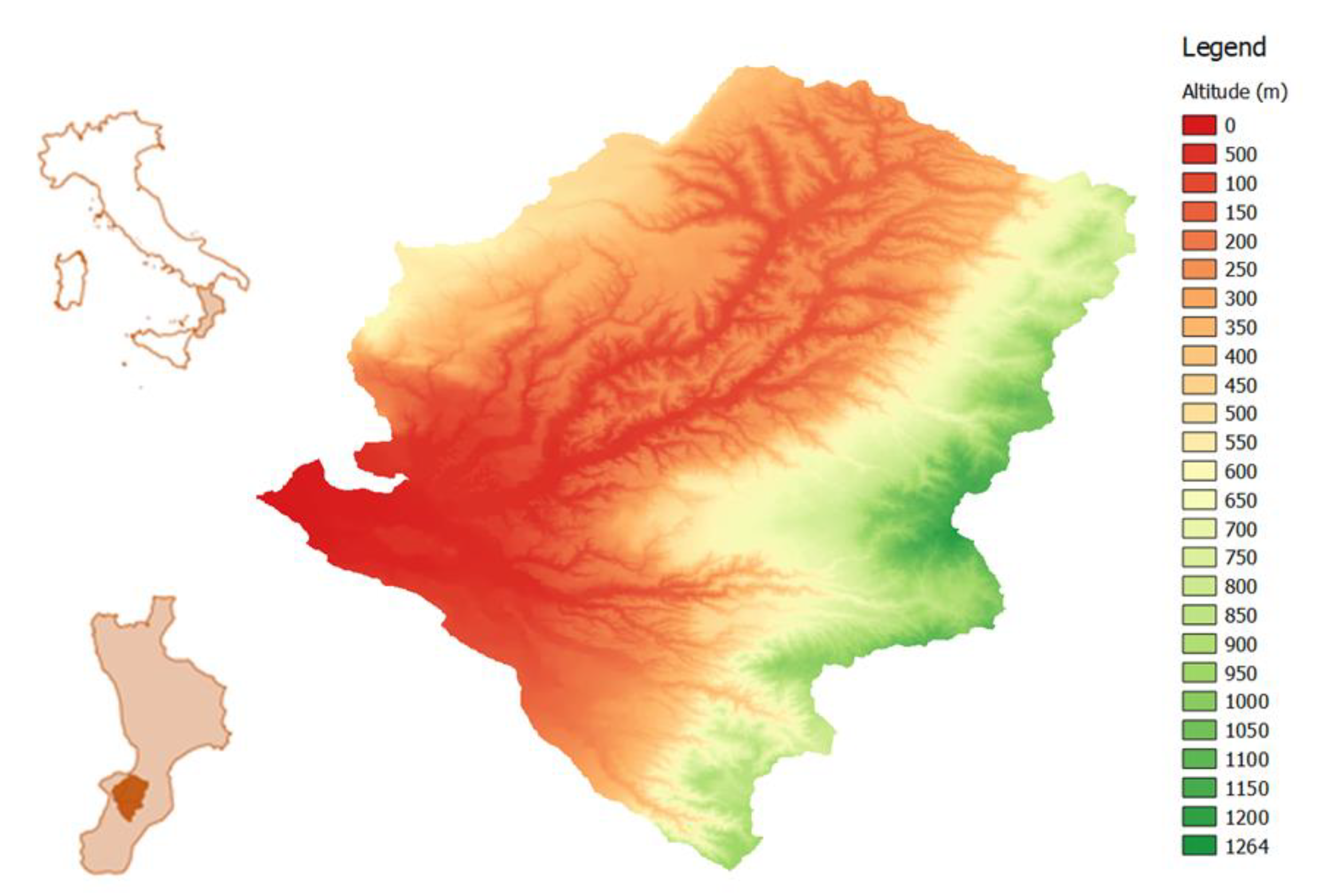
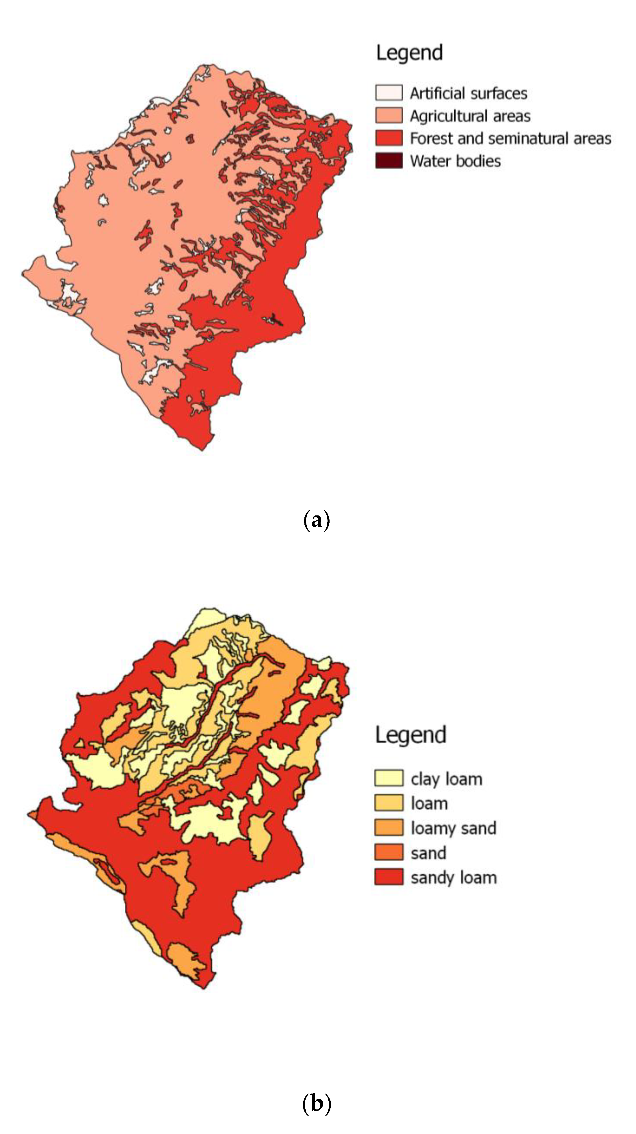
3.2. The Sample Watershed (Mesima Torrent, Southern Italy)

The four models were applied to the watershed of Mesima torrent, Calabria, Southern Italy (Figure 2) has an ellipsoidal shape (Gravelius index of 1.5) with a perimeter of 152 km and covers an area of 795 km². The torrent sources in the Serre mountain system at 1245 m a.s.l. and, running along 43 km, flows into the Tyrrhenian Sea; the outlet is located close to the town of Rosarno (38.5006° N, 15.9875° E). The mean altitude and slope steepness are 395 m and 29%, respectively. According to [56], the watershed concentration time (that is, the time required by runoff to reach the closure section from the farthest hydraulically distant point [57]) is estimated in about 12 h.

The climate of the watershed is semi-arid (Csa type, according to Koppen-Geiger’s classification [58]), typical of the Mediterranean Basin. Winter is generally mild and wet and summer is hot and dry. The average precipitation is 900 mm/y, distributed mainly in autumn and winter; snow is practically absent, except for some days in the highest mountains. The average minimum and maximum temperatures are 4.2 and 31.8 °C, respectively (meteorological station of Arena, 38.5613° N, 16.2166° E).

According to the “Corine Land Cover” classification (scale 1:100,000, 2007) shown in Figure 3a, the main land use in the watershed is agricultural (66% of the total area) with intensive crops (mainly vegetables), olive groves and other fruit orchards (citrus and kiwi fruit). Forest areas cover 31% of the total area, while the remaining part of the watershed is covered by urban areas (3%, Figure 3a). Soil texture, derived from the ‘Soil Map of the Calabria Region’ (scale 1:250,000 [59]), is prevalently sandy loam (50% of the basin area), with loam (19%) and clay loam (18%) zones in the remaining areas [60] (Figure 3b). The soils have a low runoff potential when thoroughly wet [21].

A 20-m resolution Digital Elevation Model (DEM), provided by ISPRA (Environmental Research and Protection Higher Institute of Italy), was used to divide the watershed into interconnected subwatersheds for the spatially distributed models and simulate the stream network using GIS software (QuantumGIS). A more detailed discretisation was not made given that the available land use and soil texture maps have a lower resolution compared to the DEM (Figure 3). Using the GIS software, the maps of land use and soil type were overlaid, to input the geomorphological information to the models. Therefore, each subwatershed was characterised by specific land use and soil type, on which its hydrological response depends.

For the hydrological and hydraulic simulation using the WEC-FLOOD model, a computational mesh of 39,385 elements and 19,921 nodes has been generated, covering the whole watershed. Mesh node elevations have been computed by interpolating the elevations of the DEM cell centres. A bilinear approximation was adopted inside the rectangular area within the centres of four neighbour cells of the original DEM model, sharing a common node.

3.3. The Hydrological Database

The hydrological database which was used to analyse the software was provided by the Regional Agency for Environmental Protection of Calabria covers the period of January 2008 to May 2011 and contains: (i) hourly rainfall, collected at 16 rain gauging stations (five inside the watershed and nine within a maximum distance of 15 km); (ii) surface water discharge, measured every 20 min by an ultrasonic flow metre at the outlet.

In the hourly rainfall series of the experimental database, two consecutive events were considered separately, if no rainfall was recorded for 6 h or more [61]. For the model evaluation, 10 rainfall–rainfall events were identified (Table 1). In order to spatially scale the rainfall input, Thiessen’s polygon method [62] was applied: 15 polygons were drawn covering the entire basin area.

The rainfall depths measured for the 10 experimental events were in the range 43–525 mm (

Table 2. Hydrological characterisation of the 10 rainfall–runoff events used for model verification in the Mesima torrent (Calabria, Southern Italy).

Rainfall/Runoff Event	Rainfall				Runoff
	Total Depth (mm)	Duration (h)	Intensity (mm/h)		Total Volume (mm)	Runoff Coefficient (−)	Peak (m3/s)	Time to Peak (h)
			Average	Max
1–6 December 2008	261	63	3.3	24.8	11.94	4.58	195	38
10–15 January 2009	375	104	3.3	29.7	20.82	5.55	272	60
24–31 January 2009	277	169	1.5	9.9	24.95	9.01	125	115
9–12 November 2009	184	85	2.2	28.2	20.34	11.03	235	50
5–18 February 2010	525	304	1.7	169.2	40.91	7.79	169	73
6–11 March 2010	292	95	2.8	22.1	33.58	11.49	323	83
17–22 October 2010	370	104	3.1	28.0	38.43	10.39	427	44
1–3 November 2010	226	29	5.4	530.8	30.54	13.52	531	17
30 January–4 February 2011	43	120	0.4	4.5	35.34	82.13	180	127
28 February–8 March 2011	331	169	1.7	279.2	13.57	4.10	279	35

Notes: the events reported in bold or in italics were used for model calibration or validation, respectively.

). The latter was generated by the longest event which occurred from 5 to 18 of February 2010 (304 h) and produced the highest runoff volume (40.91 mm). The highest peak discharge was observed from 1 to 3 November 2010 (531 m³/s), which was also characterised by the highest rainfall intensity (mean 5.4 mm/h and maximum 531 mm/h), as the quickest watershed’s response (time to peak of only 17 h) to a very short rainfall event (29 h). The event recorded from 30 January to 4 February 2011 had the lowest rainfall intensity (mean 0.4 mm/h and maximum 4.5 mm/h), but generated the highest runoff coefficient (82.1%), since it occurred on completely saturated soil, due to the antecedent precipitation. Moreover, for this event, the flood peak was very delayed (107 h) compared to the start of the precipitation. Finally, the lowest runoff coefficient was observed from 28 February to 8 March 2011 (4.10%), while the lowest peak discharge which was recorded occurred from 24 to 31 January 2009 (125 m³/s, Table 2).

3.4. Calibration and Validation Procedures

The split-sample technique [63] was used to evaluate the runoff volume predicted by the software during the calibration and validation stages. More specifically, four of the 10 available rainfall–runoff events observed at the watershed outlet were chosen for calibration. Of these events, three involved dry, medium water content and wet soils, due to antecedent precipitation (Antecedent Moisture Content of the SCS-CN method, AMC I, II and III), and the fourth event was randomly selected those in which the subwatersheds had different water contents. The remaining six events were used for model validation. This was done in order to avoid the bias of events that were too dry or too wet [21].

The hydrological components were calibrated by varying the input parameters to which discharge is more sensitive. The choice of these input parameters was done considering the results of the sensitivity analysis carried out by several authors for the considered hydrological models [37,38,39,64,65,66,67,68]. During the calibration phase, these parameters were modified for each event until the best prediction of the peak discharge was obtained. The subsequent subsection gives more details about the calibration of each model.

HEC-HMS used the SCS-CN method as an infiltration model to calculate the runoff volume to be routed along the torrent channels. The four events used for model calibration were those which occurred from 1 to 6 December 2008 (AMC II), 5–18 February 2010 (AMC II), 6–11 March 2010 (AMC I-II) and 30 January–4 February 2011 (AMC III). The resulting calibrated CNs (averaged among the three subwatersheds, in which the Mesima torrent was divided) were 50.6, 70.9, 57.4, 84.9, respectively.

MIKE11 NAM was autocalibrated [48]. The autocalibration routine “AutoCal” of MIKE includes nine parameters of the rainfall–runoff algorithm [69]. The autocalibration procedure is based on a multiobjective optimisation strategy, in which four calibration objectives (the overall volume error, RMSE, and both average RMSE of peak and low flow events) are considered [48]. The user determines which of these objectives should be considered in the autocalibration routine. In our study, the calibration procedure stopped when the maximum coefficient of efficiency value (E), calculated on the basis of RMSE according to [27], is achieved (see also Section 2.2). Then, using the calibrated parameters, the model was applied to the events of the validation stage.

SWMM used the SCS-CN method [70] in the Runoff block for the rainfall–runoff transformation. As regards the Transport block, the flood wave propagation was simulated using Clark’s unit hydrograph linear model. In the calibration phase, the event of 6–11 March 2010 was used considering the Antecedent Moisture Condition II, while, for AMC I and AMC III, the events of 1–6 December 2008 and 30 January–4 February 2011 were chosen; as the fourth event the rainfall/runoff of 5–18 February 2010 (AMC II) was used. The calibrated values of CNs were 52 for AMC II, 47 for AMC I and 70 for AMC III.

WEC-FLOOD was calibrated by setting up the input parameters related to water loss after rainfall. The Horton method was used as the infiltration model, increasing the parameters of the infiltration curve from zero infiltration to the optimal values. The initial infiltration was between 4.3 (event of 5–18 February 2010) and 6.8 (1–6 December 2008) mm/h, while the final value was in the range of 3.3 (6–11 March 2010) and 4.7 (1–6 December 2008) mm/h. The decaying rate was set to 0.65 for the event of 6–11 March 2008) and 0.75 h⁻¹ (1–6 December 2008 and 5–18 February 2010). For the event of 30 January–4 February 2011, all these input parameters had to be set to zero, otherwise the model would not have produced runoff.

4. Results and Discussions

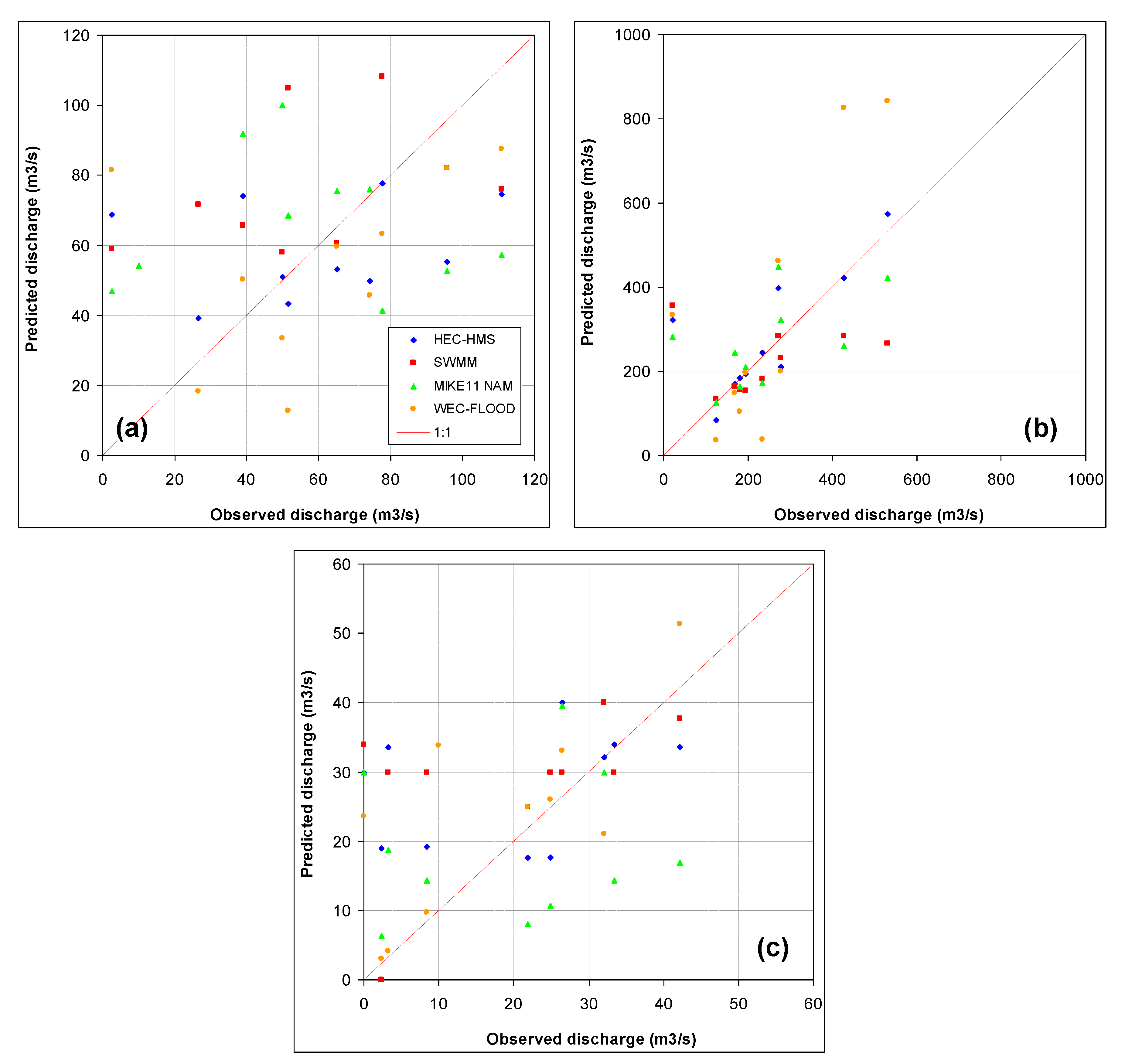
4.1. Analysis of the Discharge Prediction Capability

By a visual comparison, the mean, minimum and maximum values of the observed versus predicted discharges appear quite scattered compared to the identity line (prediction equal to the observation) as shown in Figure 4. The maximum value of the discharges predicted using the HEC-HMS software, which lined up quite well along the 1:1 l (Figure 4b) is an exception.

During the calibration phase, a slight tendency to underestimate the water discharge measured at the outlet of the experimental watershed was noticed for three models (SWMM, MIKE11 NAM and WEC-FLOOD), as shown by the positive value of CRM (<0.04,

Table 3. Statistics and indexes for evaluating the discharge (in m³/s) prediction capability of four hydrological models in the Mesima torrent (Calabria, Southern Italy).

Water Discharge	Mean	Standard Deviation	Minimum	Maximum	R2	E	E*	RMSE	CRM
HEC-HMS
Calibration
Observed	58.7	41.0	26.6	216.8	0.76	0.60	0.36	41.93	−0.01
Simulated	54.0	40.0	31.7	224.8
Difference (%)	−8.0	−2.4	18.9	3.7
Validation
Observed	70.2	69.5	19.7	311.3	0.62	0.44	0.27	72.71	0.05
Simulated	58.0	64.3	27.0	322.2
Difference (%)	−17.4	−7.5	37.0	3.5
SWMM
Calibration
Observed	216.8	71.6	169.2	323.0	0.45	0.38	0.15	22.55	0.03
Simulated	209.5	64.6	153.6	282.8
Difference (%)	−3.4	−9.7	−9.2	−12.4
Validation
Observed	311.3	144.8	124.7	530.8	0.57	0.08	0.21	40.62	0.26
Simulated	230.5	60.9	134.5	284.5
Difference (%)	−26.0	−57.9	7.9	−46.4
MIKE11 NAM
Calibration
Observed	216.8	71.6	169.2	323.0	0.97	0.93	0.70	7.60	0.01
Simulated	214.1	84.6	148.2	334.8
Difference (%)	−1.3	18.2	−12.4	3.6
Validation
Observed	311.3	144.8	124.7	530.8	0.38	0.27	0.17	36.18	0.06
Simulated	291.4	130.1	126.1	447.1
Difference (%)	−6.4	−10.1	1.1	−15.8
WEC-FLOOD
Calibration
Observed	216.8	71.6	169.2	323.0	0.73	0.52	0.43	19.89	0.04
Simulated	208.8	92.4	103.3	328.4
Difference (%)	−3.7	29.1	−39.0	1.7
Validation
Observed	311.3	144.8	124.7	530.8	0.84	−2.30	−0.89	77.16	−0.29
Simulated	401.3	369.9	36.9	842.2
Difference (%)	28.9	155.5	−70.4	58.7

). Conversely, HEC-HMS tended to overestimate the discharge (CRM = −0.01). Of all the evaluated models, the MIKE11 NAM model gave the best performance in predicting the discharge. Very high values of both R² (equal to 0.97) and E (0.93) were achieved, and the mean and maximum discharges predicted by NAM were very close to the corresponding observations, with differences of −1.3% and +3.6%, respectively. HEC-HMS and WEC-FLOOD gave satisfactory values of E (0.60 and 0.52, respectively), although the RMSE index was quite high for HEC-HMS (>half standard deviation of the observed discharge). For these models, the differences between predictions and observations of mean and maximum discharges remained quite limited (not higher than −8.0% and +3.7%, respectively, Table 3).

For SWMM, the value of E was just acceptable (0.38), and the predicted maximum discharge was lower than the observed values (−12.4%), although the mean values were close to each other (−3.4%, Table 3).

Clearly, the performance at the validation stage is lower than that obtained during the calibration stage. Specifically, only HEC-HMS provided acceptable values of E (0.60) and E* (0.36), and a slight underestimation of discharge was recorded (CRM = 0.05); for this model, the differences between the mean and maximum observed and predicted discharges remained quite limited (<17.4%), except for the minimum value (with a difference of +37.0%). Conversely, the model efficiencies E and E*, were lower for SWMM (equal to 0.08 and 0.21, respectively) and MIKE11 NAM (0.27 and 0.17), and even negative for WEC-FLOOD (E = −2.30 and E* = −0.89). MIKE11 NAM reveals a slight tendency to underestimate (CRM = 0.06), while, for SWMM and WEC-FLOOD the differences were larger and always higher than 25% with peaks error for the maximum discharge of −46.4% and +58.7%, respectively. These differences were due to the tendency to underestimate, like in the case of SWMM or overestimate (WEC-FLOOD) the observed events as shown by the high deviation of CRMs from zero (+0.26, SWMM, and −0.29, WEC-FLOOD, Table 3).

The discharge prediction capability was compared with other modelling experiences carried out in semi-arid watersheds, available in the literature. As regards the HEC-HMS model, the peak discharge was better estimated using the “Initial and Constant” method (E = 0.90–0.95) than the “SCS-CN” method (E = 0.30) in Southern Italy [20]. The model efficiency detected by [71] in applying the model in an Israeli watershed was in the range 0.90–0.97. In a semi-urbanised watershed in Texas (USA), [72] reported errors of about 30% in predicting the peak discharge, after model calibration. Deviations lower than 4%, were found by [73] in a semi-arid watershed of Pakistan when comparing observed and calibrated peak flows.

Fewer study cases, which are suitable for comparison with the experimental watershed of this study, are available in the literature for the SWMM and MIKE11 NAM software. The first software was mostly used to predict floods in urban watersheds rather than in rural areas; often, its performance was compared to those provided by the MIKE-family models. For instance, in two small urban watersheds in the city of Athens (Greece) and in West Bengal (India), respectively, [74,75] found that the 1D model, which is obviously faster than the 1D–2D model, was not able to simulate the flood extent and inundation as accurately. SWMM was used in another Italian watershed, where the model performed well in simulating runoff (E = 0.81) [51]. In Australia, SWMM was very accurate in simulating the peak discharge with average errors of around 5% [76]. [77] found errors of up to 31% in the simulated values of the discharge in four peri-urban watersheds of Southern Brazil. In a large urban watershed of Southern California (USA), the predicted peak flows were overestimated by 4–25% compared to the observed values [78]. MIKE11 NAM was calibrated and validated in a Greek watershed by [79], who detected E values of between 0.59 and 0.80. The automatic calibration routine of MIKE11 NAM was used also by [80], to optimise the parameter values for Fitzroy Catchment (Australia); the authors obtained a good agreement between the observed and simulated hydrographs. Satisfactory results were reported by [81], who predicted discharges in the Sarisoo River (Iran) using the automatic calibration procedure of the model. [82] simulated the rainfall–runoff transformation in the Nzhelele River (South Africa) using MIKE11 in autocalibration mode using the root mean square error (RMSE) as an objective function. The WEC-FLOOD applications in the semi-arid environments were even more limited compared to the other three models, because the model is still at the early stage of development and dissemination. However, WEC-FLOOD was tested by the developers, comparing its capability to couple 1D and 2D approaches with several hydrodynamic models, at both the academic and professional applications [38]. A good agreement between the WEC-FLOOD results with observed data and literature results were found. The advantages of using a diffusive model as WEC-FLOOD, in terms of computational efficiency and robustness, are evident.

Comparing the hydrographs generated by the four models to the observed discharge, HEC-HMS software is the most accurate in simulating the temporal evolution of the floods. This software reproduced the events of the calibration phase with satisfactory accuracy (except for the concentration limb of the event dated 1–6 December 2008), since the observed and simulated hydrographs were in close agreement with each other.

Conversely, SWMM failed to reliably simulate the peak discharge observed in all four events. A basic inaccuracy in predicting the runoff event following the rainfall recorded between 5 and 18 February 2000 was also noticed for this model and for WEC-FLOOD (Figure 5).

Confirming what was highlighted by the quantitative analysis of the discharge prediction accuracy (Table 3), for the events of the validation phase, noticeable differences between the predicted and observed discharges were noticed for the four models. However, HEC-HMS was quite accurate in simulating the events of 9–12 November 2009 and 1–3 November 2010, while MIKE performed better in reproducing the hydrographs dated 17–22 October 2010 (in which the simulating peak occurred earlier than the observed value) and 28 February–8 March 2011. The hydrographs predicted by SWMM were similar to those observed for the events 28 February–8 March 2011. Conversely, a large inaccuracy in simulating the observed floods was detected for the WEC-FLOOD model, which did not even simulate discharge over the baseflow for the events of 24–31 January 2009, 9 or 12 November 2009, and largely overestimated the floods that occurred in 10–15 January 2009, 17–22 October 2010 and 1–3 November 2010 (Figure 5).

It should be noticed that the runoff events characterised by several flood peaks in response to impulsive precipitation were simulated with low accuracy by all models (e.g., the events of 5–18 February 2010, 24–31 January 2009 and 28 February–8 March 2011), also for the calibration period (Figure 5). Overall, this detailed analysis allows some considerations to be drawn about the performance and the best choice of the evaluated models.

Firstly, the higher accuracy in reproducing the observed discharges detected for HEC-HMS is quite expected, since this model works on an event scale, where the water content of the soil is updated at the start of each event.

Secondly, the difficulty that the continuous models (SWMM and WEC-FLOOD) had in updating the humidity conditions of the soil is quite surprising as they were expected to adjust to these conditions by applying the mass conservation equations. This difficulty has been also detected by other authors working with continuous models based on the SCS-CN method. For instance, [83,84] noticed that the AnnAGNPS model was not always successful in modelling the water balance of soil. This constraint could be overcome in SWMM using different CNs, for instance, on a seasonal basis.

Thirdly, the benefit of calibration was evident for the conceptual models (HEC-HMS and MIKE11 NAM). The other physical-based models, SWMM and WEC-FLOOD, do not require calibration, since they are based on mass and momentum conservation equations [3,7,12]. Given that the data requirements of any model drastically increase with the complexity of the model [3], the use of simpler conceptual models (such as HEC-HMS and MIKE11 NAM), which require fewer input parameters, is recommended in environmental conditions similar as the studied watershed. HEC-HMS appears to be the best choice, since this model (like the more complex MIKE11 NAM) has a lumped spatial scale. This model characteristic better fits to rather homogenous watersheds (particularly in terms of land use) as the Mèsima torrent than watersheds with several land uses or soils of different hydrological properties, which are better predicted by distributed models.

Fourthly and finally, the poor performance of the WEC-FLOOD model, which is based on Horton’s infiltration method, is unexpected in a watershed of a semi-arid environment, which is dominated by the infiltration-excess mechanism for runoff generation [85], where reliable values of the soil hydraulic conductivity are needed for accurate predictions. This result may be attributable to the lack of measurements of the infiltration capability of the soil, which has forced the modellers to calibrate the model, achieving in some case unrealistic parameters (infiltration modelled as zero).

4.2. Analysis of the Model’s Performance Matrix

According to the opinions given by those interviewed, the input requirement and prediction accuracy, to which scores equal to 4.9 and 4.7, respectively, were attributed, are the most important requisites and performances of a hydrological model (

Table 4. Mean weight given by the interviewed people to the 10 parameters used for calculating the software evaluation matrix.

Parameter	Mean Weight
	(0 to 5)				(0 to 1)
	Researchers	Freelancers	Public Administration Officials	Mean Among Stakeholder Categories
Input requirement	4.7	5.0	4.9	4.9	1.0
Availability of input data	2.7	3.2	1.3	2.3	0.5
Complexity	4.3	4.7	3.6	4.1	0.8
User interface	4.2	4.3	3.5	4.0	0.8
Prediction accuracy	5.0	4.5	4.6	4.7	0.9
Range of time and space scales	2.2	3.0	1.9	2.3	0.5
Flexibility	1.8	2.3	0.8	1.6	0.3
Computation effort	4.0	3.0	2.8	3.2	0.6
Commercial cost	1.8	3.2	1.6	2.1	0.4
Compatibility with other software	3.7	4.0	1.6	3.0	0.6

). Of course, the simplicity of model implementation and the quality of its output were considered extremely important, particularly for the public administration officials (input requirement score = 4.9) and researchers (prediction accuracy score = 5.0). Additionally, the availability of a user-friendly interface and the low complexity are appreciated by the users (scores of 4.0 and 4.1), especially by the freelancers (scores of 4.3 and 4.7, respectively). Conversely, the lowest scores were attributed to the model flexibility (1.6), cost (2.1) and availability of input data (2.3, Table 4), presumably because: (i) the users—particularly the public administration officials—need to perform various tasks (for instance erosion predictions or water quality forecasts) and thus are open to change the software, when a different and specific task is required; (ii) most of the interviewed people work in a public administration (e.g., local administration or university), where finances are less limited compared to freelancers; (iii) the modellers, especially the academics, are able to easily measure or accurately estimate the input parameters required by the models, rather than trusting to literature or manual data. It is worth noticing that the computation effort is not a strict requisite according to the stakeholders’ opinion (score = 3.2), in particular for the public administration officials (score of 2.8) and freelancers (3.0). This may be quite surprising, since, when the flood maps are required as model predictions, the computation times of 2D models (such as the models of the MIKE-family and WEC-FLOOD) can be high and this may be a limitation for a model [5].

The authors have attributed different scores to the software evaluated in this study regardless of its performance/requisite. As shown in

Table 5. Scores for the 10 parameters used for calculating the model evaluation matrix of the four hydrological computer models implemented in the Mesima torrent (Calabria, Southern Italy).

Model Performance/Requisite	Software
	HEC-HMS	SWMM	MIKE11 NAM	WEC-FLOOD
Input requirement	0.6	0.6	0	0.7
Availability of input data	0.6	0.6	0.6	0.6
Complexity	0.6	0.6	1	0.4
User interface	1	1	1	1
Prediction accuracy	0.6	0.1	0.7	0
Range of time and space scales	0.4	1	1	0.4
Flexibility	0.6	0.6	0.6	1
Computation effort	1	1	1	0.5
Commercial cost	1	1	0	0.5
Compatibility with other software	0.5	0.5	1	0.8
TOTAL	6.9	7.0	6.9	5.9

, the standardised scores range from 0 to 1. For the models evaluated in this study, MIKE 11 NAM required 14 input parameters, HEC-HMS six, SWMM five and finally WEC-FLOOD four. The model performance related to this evaluation criterion is 0 for MIKE 11 NAM, 0.6 for SWMM and HEC-HMS, and 0.7 for WEC-FLOOD. With regard to the “availability of input data”, there are very few differences between the performance of the four models, since all the input data required can be collected very easily for all the models. Concerning the “complexity”, the model implementation in the studied watershed required the watershed parameterisation, the input setting, the calibration of the parameters and the other operations needed to run the software. All these operations were quite fast for three models (HEC-HMS, SWMM and MIKE 11 NAM), but not for WEC-FLOOD. For this model, the watershed parametrisation was more difficult than in the others. This was due to the intrinsic characteristic of the solver, which couples the 1D simulation in the channels with the 2D simulation in the floodplains. MIKE 11 NAM got the highest score for this parameter, thanks to its autocalibration routine, despite the greatest number of input data.

All the models, including WEC-FLOOD, which was developed in a scholar environment, have a user-friendly interface running in Windows, OSx and Linux platforms.

Regarding the “prediction accuracy” MIKE 11 NAM and HEC-HMS showed the best performance (scores of 0.7 and 0.6, respectively), while the prediction accuracies of SWMM and WEC-FLOOD were very low (0.1 and 0, respectively). Since SWMM and MIKE 11 NAM work in continuous simulation, these models performed better than the lumped and event-based models (HEC-HMS and WEC-FLOOD) for the parameter “range of time and space scales”, WEC-FLOOD is able to provide more information about the water flow, which is typical of 2D simulations and therefore its score was much higher than the other three models (1 vs 0.6). The “computation effort” was very low for all models, except for WEC-FLOOD, which, as expected, required more time to complete simulations. This is due to the computational time that depends on the set time resolution, the number of cells in watershed discretisation and the duration of the simulated event. The “commercial cost” of the software scored from 0 (MIKE 11 NAM, which is a commercial code) to one for the freeware software (SWMM and HEC-HMS). WEC-FLOOD should not be evaluated, because it is an academic model that it is not still available. However, in order to complete the performance matrix and to take into account the possibilities of it becoming a freeware or commercial code in the future, a medium (0.5) score was attributed to WEC-FLOOD. With reference to the last parameter (“compatibility with other software”), the highest score was attributed to MIKE11 NAM for its compatibility not only with GIS software, but also with the other models of the MIKE-family, followed by WEC-FLOOD, whose solver is integrated into freeware GIS software.

According to the weighted scores, HEC-HMS (4.45) and MIKE 11 NAM (4.43) performed the best for the case study, with a score difference of only 0.02 (

Table 6. Weighted scores for the 10 parameters used for calculating the model evaluation matrix of the four hydrological computer models tested in the Mesima torrent (Calabria, Southern Italy).

Model Performance/Requisite	Software
	HEC-HMS	SWMM	MIKE11 NAM	WEC-FLOOD
Input requirement	0.55	0.62	0	0.69
Availability of input data	0.27	0.27	0.27	0.27
Complexity	0.49	0.49	0.82	0.33
User interface	0.79	0.79	0.79	0.79
Prediction accuracy	0.61	0.05	0.67	0
Range of time and space scales	0.18	0.46	0.46	0.18
Flexibility	0.19	0.19	0.19	0.32
Computation effort	0.64	0.64	0.64	0.32
Commercial cost	0.42	0.42	0	0.21
Compatibility with other software	0.30	0.30	0.59	0.47
TOTAL	4.45	4.23	4.43	3.59

). On the total weighted score of HEC-HMS, the “prediction accuracy” and the “computation effort” (>0.60), as well as the “user interface” (>0.70), weighed positively, while the “range of time and space scales”, due to the fact that the model is lumped and event-based, reduced the score. Conversely, the overall performance of MIKE11 NAM was lowered by its commercial cost and the high number of inputs required. SWMM totalled a score by only 0.2 less than MIKE, because of its lower accuracy hindered by the model’s tendency to underestimate the flood peak. The challenging potential of the WEC-FLOOD model is evident from this analysis since its score is very close to the performance of the other three well-known and commonly used models (Table 6).

5. Conclusions

This study proposed a criterion to evaluate the performance and overall user experience of hydrological software. The method was tested with four hydrological computer models (HEC-HMS, SWMM, MIKE 11 NAM and WEC-FLOOD), used to predict the water discharge at the outlet of a Mediterranean torrent. The case study was a semi-arid watershed in Southern Italy. The computer programs were chosen in order to cover many aspects both from a mathematical point of view (physical-based, conceptual, lumped-parameter or distributed-parameter) and commercial feasibility.

The models were calibrated and then validated using four and six rainfall–runoff events, respectively. The evaluation of the “prediction accuracy” which featured several indicators, commonly used in the hydrological literature, showed a slight peak flow underestimation for HEC-HMS (CRM = 0.05) and MIKE11 NAM (CRM = 0.06), while SWMM (CRM = +0.26) and WEC-FLOOD (CRM = −0.29) underestimated and overestimated the observed events, respectively.

In addition to the accuracy in predicting discharge, the evaluation of the models was extended to other performances and requisites, using a “performance” matrix based on 10 parameters weighted through stakeholders’ and users’ interviews. According to this matrix, HEC-HMS and MIKE 11 NAM were the best models in the case study, thanks to their low complexity and computation effort, as well as the good user interface and prediction accuracy. However, the performance of the MIKE11 NAM model was hindered by its cost and by the high number of parameters. The score of SWMM was strongly affected by the lower prediction accuracy, which put the model in third place. The lower performance of WEC-FLOOD can be justified by the fact that the model is in the early stage of development in comparison to the other well-consolidated models.

Overall, the proposal of the performance matrix for hydrological models, which has been one of the aims of this study, may represent a first step in building a more complete evaluation framework of the hydrological and hydraulic commercial models, in order to give indications to allow potential users to make an optimal choice.

References

1. De Vente, J.; Poesen, J. Predicting soil erosion and sediment yield at the basin scale: Scale issues and semi-quantitative models. Earth Sci. Rev. 2005, 71, 95–125. [Google Scholar] [CrossRef]
2. Bisantino, T.; Bingner, R.; Chouaib, W.; Gentile, F.; Liuzzi, G.T. Estimation of Runoff, Peak Discharge and Sediment Load at the Event Scale in a Medium-Size Mediterranean Watershed Using the AnnaGNPS Model. Land Degrad. Dev. 2015, 26, 340–355. [Google Scholar] [CrossRef]
3. Aksoy, H.; Kavvas, M.L. A review of hillslope and watershed scale erosion and sediment transport models. Catena 2005, 64, 247–271. [Google Scholar] [CrossRef]
4. Singh, V.P.; Woolhiser, D.A. Mathematical Modeling of Watershed Hydrology. J. Hydrol. Eng. 2002, 7, 270–292. [Google Scholar] [CrossRef] [Green Version]
5. Filianoti, P.G.; Nicotra, A.; Labate, A.; Zema, D.A. A Method to Improve the Flood Maps Forecasted by On-Line Use of 1D Model. Water 2020, 12, 1525. [Google Scholar] [CrossRef]
6. Borah, D.K.; Bera, M. Watershed-scale hydrologic and nonpoint-source pollution models: Review of applications. Trans. ASAE 2004, 47, 789–803. [Google Scholar] [CrossRef] [Green Version]
7. Merritt, W.; Letcher, R.; Jakeman, A.J. A review of erosion and sediment transport models. Environ. Model. Softw. 2003, 18, 761–799. [Google Scholar] [CrossRef]
8. Lieskovský, J.; Kenderessy, P. Modelling the effect of vegetation cover and different tillage practices on soil erosion in vineyards: A case study in vráble (slovakia) using watem/sedem. Land Degrad. Dev. 2012, 25, 288–296. [Google Scholar] [CrossRef]
9. Cao, L.; Zhang, K.; Dai, H.; Liang, Y. Modeling interrill erosion on un-paved roads in the Loess Plateau of China. Land Degrad. Dev. 2015, 26, 825–832. [Google Scholar] [CrossRef]
10. Liebe, J.R.; Van De Giesen, N.; Andreini, M.; Walter, M.T.; Steenhuis, T.S. Determining watershed response in data poor environments with remotely sensed small reservoirs as runoff gauges. Water Resour. Res. 2009, 45, 7369. [Google Scholar] [CrossRef] [Green Version]
11. Saliha, A.H.; Awulachew, S.B.; Cullmann, J.; Horlacher, H.-B. Estimation of flow in ungauged catchments by coupling a hydrological model and neural networks: Case study. Hydrol. Res. 2011, 42, 386–400. [Google Scholar] [CrossRef]
12. Fu, B.; Merritt, W.; Croke, B.F.; Weber, T.R.; Jakeman, A.J. A review of catchment-scale water quality and erosion models and a synthesis of future prospects. Environ. Model. Softw. 2019, 114, 75–97. [Google Scholar] [CrossRef]
13. Martın-Vide, J.; Niñerola, D.; Bateman, A.; Navarro, A.; Velasco, E. Runoff and sediment transport in a torrential ephemeral stream of the Mediterranean coast. J. Hydrol. 1999, 225, 118–129. [Google Scholar] [CrossRef]
14. Zema, D.A.; Bombino, G.; Boix-Fayos, C.; Tamburino, V.; Zimbone, S.M.; Fortugno, D. Evaluation and modeling of scouring and sedimentation around check dams in a Mediterranean torrent in Calabria, Italy. J. Soil Water Conserv. 2014, 69, 316–329. [Google Scholar] [CrossRef]
15. Llasat, M.-C.; Marcos, R.; Turco, M.; Gilabert, J.; Llasat-Botija, M. Trends in flash flood events versus convective precipitation in the Mediterranean region: The case of Catalonia. J. Hydrol. 2016, 541, 24–37. [Google Scholar] [CrossRef] [Green Version]
16. Fortugno, D.; Boix-Fayos, C.; Bombino, G.; Denisi, P.; Rubio, J.M.Q.; Tamburino, V.; Zema, D.A. Adjustments in channel morphology due to land-use changes and check dam installation in mountain torrents of Calabria (southern Italy). Earth Surf. Process. Landf. 2017, 42, 2469–2483. [Google Scholar] [CrossRef]
17. Zema, D.A.; Bombino, G.; Denisi, P.; Lucas-Borja, M.E.; Zimbone, S.M. Evaluating the effects of check dams on channel geometry, bed sediment size and riparian vegetation in Mediterranean mountain torrents. Sci. Total Environ. 2018, 642, 327–340. [Google Scholar] [CrossRef] [PubMed]
18. Bombino, G.; Gurnell, A.M.; Tamburino, V.; Zema, D.A.; Zimbone, S.M. A method for assessing channelization effects on riparian vegetation in a Mediterranean environment. River Res. Appl. 2007, 23, 613–630. [Google Scholar] [CrossRef]
19. Boix-Fayos, C.; Barberá, G.G.; López-Bermúdez, F.; Castillo, V.M. Effects of check dams, reforestation and land-use changes on river channel morphology: Case study of the Rogativa catchment (Murcia, Spain). Geomorphology 2007, 91, 103–123. [Google Scholar] [CrossRef]
20. Zema, D.A.; Labate, A.; Martino, D.; Zimbone, S.M. Comparing Different Infiltration Methods of the HEC-HMS Model: The Case Study of the Mésima Torrent (Southern Italy). Land Degrad. Dev. 2017, 28, 294–308. [Google Scholar] [CrossRef]
21. Zema, D.A.; Lucas-Borja, M.E.; Carrà, B.G.; Denisi, P.; Rodrigues, V.A.; Ranzini, M.; Arcova, F.C.S.; De Cicco, V.; Zimbone, S.M. Simulating the hydrological response of a small tropical forest watershed (Mata Atlantica, Brazil) by the AnnAGNPS model. Sci. Total. Environ. 2018, 636, 737–750. [Google Scholar] [CrossRef] [PubMed] [Green Version]
22. Harmel, R.; Smith, P.; Migliaccio, K.W.; Chaubey, I.; Douglas-Mankin, K.; Benham, B.; Shukla, S.; Muñoz-Carpena, R.; Robson, B.J. Evaluating, interpreting, and communicating performance of hydrologic/water quality models considering intended use: A review and recommendations. Environ. Model. Softw. 2014, 57, 40–51. [Google Scholar] [CrossRef]
23. Singh, G.; Kumar, E. Input data scale impacts on modeling output results: A review. J. Spat. Hydrol. 2017, 13, 1–10. [Google Scholar]
24. Willmott, C.J. Some comments on the evaluation of model performance. Bull. Am. Meteorol. Soc. 1982, 63, 1309–1313. [Google Scholar] [CrossRef] [Green Version]
25. Legates, D.R.; McCabe, G.J. Evaluating the use of “goodness-of-fit” Measures in hydrologic and hydroclimatic model validation. Water Resour. Res. 1999, 35, 233–241. [Google Scholar] [CrossRef]
26. Loague, K.; Green, R.E. Statistical and graphical methods for evaluating solute transport models: Overview and application. J. Contam. Hydrol. 1991, 7, 51–73. [Google Scholar] [CrossRef]
27. Nash, J.E.; Sutcliffe, J.V. River Flow forecasting through conceptual models—Part I: A discussion of principles. J. Hydrol. 1970, 10, 282–290. [Google Scholar] [CrossRef]
28. Krause, P.; Boyle, D.P.; Base, F. Comparison of different efficiency parameters for hydrological model assessment. Adv. Geosci. 2005, 5, 89–97. [Google Scholar] [CrossRef] [Green Version]
29. Moriasi, D.N.; Arnold, J.G.; Van Liew, M.W.; Bingner, R.L.; Harmel, R.D.; Veith, T.L. Model Evaluation Guidelines for Systematic Quantification of Accuracy in Watershed Simulations. Trans. ASABE 2007, 50, 885–900. [Google Scholar] [CrossRef]
30. Van Liew, M.W.; Arnold, J.G.; Garbrecht, J.D. Hydrologic simulation on agricultural watersheds: Choosing between two models. Trans. ASAE 2003, 46, 1539–1551. [Google Scholar] [CrossRef]
31. Santhi, C.; Arnold, J.G.; Williams, J.R.; Dugas, W.A.; Srinivasan, R.; Hauck, L.M. Validation of the swat model on a large rwer basin with point and nonpoint sources. JAWRA J. Am. Water Resour. Assoc. 2001, 37, 1169–1188. [Google Scholar] [CrossRef]
32. Fernández, C.; Vega, J.A.; Vieira, D.C.S. Assessing soil erosion after fire and re- habilitation treatments in NW Spain: Performance of RUSLE and revised Morgan-Morgan-Finney models. Land Degrad. Dev. 2010, 21, 58–67. [Google Scholar] [CrossRef] [Green Version]
33. Singh, J.; Knapp, H.V.; Arnold, J.; Demissie, M. Hydrological modeling of the iroquois river watershed using hspf and swat. JAWRA J. Am. Water Resour. Assoc. 2005, 41, 343–360. [Google Scholar] [CrossRef]
34. Feldman, A.D. Hydrologic Modelling System HEC-HMS, Technical Reference Manual; US Army Corps of Engineers, Hydrologic Engineering Center (HEC): Davis, CA, USA, 2000. [Google Scholar]
35. Huber, W.C.; Dickinson, R. Storm Water Management Model, Version 4: Users Manual; Environmental Research Laboratory, EPA: Washington, DC, USA, 1988. [Google Scholar]
36. Nielsen, S.A.; Hansen, E. Numerical simulation of the rainfall runoff process on a daily basis. Hydrol. Res. 1973, 4, 171–190. [Google Scholar]
37. Sinagra, M.; Nasello, C.; Tucciarelli, T.; Barbetta, S.; Massari, C.; Moramarco, T. A Self-Contained and Automated Method for Flood Hazard Maps Prediction in Urban Areas. Water 2020, 12, 1266. [Google Scholar] [CrossRef]
38. Aricò, C.; Filianoti, P.G.F.; Sinagra, M.; Tucciarelli, T. The FLO Diffusive 1D-2D Model for Simulation of River Flooding. Water 2016, 8, 200. [Google Scholar] [CrossRef] [Green Version]
39. Aricò, C.; Sinagra, M.; Begnudelli, L.; Tucciarelli, T. MAST-2D diffusive model for flood prediction on domains with triangular Delaunay unstructured meshes. Adv. Water Resour. 2011, 34, 1427–1449. [Google Scholar] [CrossRef] [Green Version]
40. Aricò, C.; Tucciarelli, T. A marching in space and time (MAST) solver of the shallow water equations. Part I: The 1D model. Adv. Water Resour. 2007, 30, 1236–1252. [Google Scholar] [CrossRef]
41. Aricò, C.; Nasello, C.; Tucciarelli, T. A marching in space and time (MAST) solver of the shallow water equations. Part II: The 2D model. Adv. Water Resour. 2007, 30, 1253–1271. [Google Scholar] [CrossRef]
42. Verma, A.K.; Jha, M.K.; Mahana, R.K. Evaluation of HEC-HMS and WEPP for simulating watershed runoff using remote sensing and geo-graphical information system. Paddy Water Environ. 2010, 8, 131–144. [Google Scholar] [CrossRef]
43. Abushandi, E.; Merkel, B. Modelling Rainfall Runoff Relations Using HEC-HMS and IHACRES for a Single Rain Event in an Arid Region of Jordan. Water Resour. Manag. 2013, 27, 2391–2409. [Google Scholar] [CrossRef]
44. Kamali, B.; Mousavi, S.J.; Abbaspour, K. Automatic calibration of HEC-HMS using single-objective and multi-objective PSO algorithms. Hydrol. Process. 2013, 27, 4028–4042. [Google Scholar] [CrossRef]
45. US Army Corps of Engineers (USACE). Hydrologic Engineering Center, Hydrologic Modelling System HEC-HMS. User’s Manual (version 4.1, July 2015). Available online: www.hec.usace.army.mil/software/hec-hms/documentation.aspx (accessed on 1 May 2020).
46. Galkate, R.V.; Jaiswal, R.K.; Thomas, T.; Nayak, T.R. Rainfall Runoff Modeling Using Conceptual NAM Model India Madhya Pradesh Map of Bina Basin up to Rahatgarh Site; Institute of Management and Technology: Nagpur, India, 2011. [Google Scholar]
47. DHI Water and Environment. 1D-2D Modelling. User Manual; DHI Water & Environment: Horsholm, Denmark, 2003. [Google Scholar]
48. DHI Water and Environment. MIKE 11: A modeling system for rivers and channels. User Guide; DHI Water & Environment: Horsholm, Denmark, 2009. [Google Scholar]
49. Razad, A.Z.A.; Sidek, L.M.; Jung, K.; Basri, H. Reservoir inflow simulation using MIKE NAM rainfall-runoff model: Case study of cameron highlands. J. Eng. Sci. Technol. 2018, 13, 4206–4225. [Google Scholar]
50. Alam, M.S.; Willems, P.; Alam, M.M. Comparative assessment of urban flood risks due to urbanization and climate change in the turnhout valley of Belgium. ABC J. Adv. Res. 2014, 3, 14–23. [Google Scholar] [CrossRef]
51. Wang, K.-H.; Altunkaynak, A. Comparative Case Study of Rainfall-Runoff Modeling between SWMM and Fuzzy Logic Approach. J. Hydrol. Eng. 2012, 17, 283–291. [Google Scholar] [CrossRef]
52. Henonin, J.; Russo, B.; Score, O.; Gourbesville, P. Real-time urban flood forecasting and modelling—A state of the art. J. Hydroinform. 2013, 15, 717–736. [Google Scholar] [CrossRef]
53. Wheater, H.S.; Jakeman, A.J.; Beven, K.J. Progress and directions in rainfall-runoff modelling. In Modelling Change in Environmental Systems; Jakeman, A.J., Beck, M.B., McAleer, M.J., Eds.; Wiley: Chichester, UK, 1993; pp. 101–132. [Google Scholar]
54. Bennett, J.P. Concepts of mathematical modeling of sediment yield. Water Resour. Res. 1974, 10, 485–492. [Google Scholar] [CrossRef]
55. Farmer, W.; Vogel, R.M. On the deterministic and stochastic use of hydrologic models. Water Resour. Res. 2016, 52, 5619–5633. [Google Scholar] [CrossRef] [Green Version]
56. Kirpich, Z.P. Time of concentration of small agricultural watersheds. Civ. Eng. 1940, 10, 362. [Google Scholar]
57. Chow, V.T. Handbook of Applied Hydrology; McGraw-Hill: New York, NY, USA, 1965. [Google Scholar]
58. Kottek, M.; Grieser, J.; Beck, C.; Rudolf, B.; Rubel, F. World Map of the Köppen-Geiger climate classification updated. Meteorol. Z. 2006, 15, 259–263. [Google Scholar] [CrossRef]
59. ARSSA Calabria (Regional Agency for Development and Services in Agriculture). Pedological Map Scale 1:250,000; Agenzia Regionale per lo Sviluppo ed i Servizi in Agricoltura della Calabria: Catanzaro, Italy, 2003. (In Italy) [Google Scholar]
60. USDA Soil Survey Staff. Soil Survey Manual; United States Department of Agriculture: Washington, DC, USA, 1975. [Google Scholar]
61. Wischmeier, W.H.; Smith, D.D. Prediction rainfall erosion losses. In Handbook No. 537; USDA: Washington, DC, USA, 1978. [Google Scholar]
62. Thiessen, A.H. Precipitation averages for large areas. Mon. Weather Rev. 1911, 39, 1082–1089. [Google Scholar] [CrossRef]
63. Klemeš, V. Operational testing of hydrological simulation models. Hydrol. Sci. J. 1986, 31, 13–24. [Google Scholar] [CrossRef]
64. Cunderlik, J.; Simonovic, S.P. Calibration, Verification and Sensitivity Analysis of the HEC-HMS Hydrologic Model; Department of Civil and Environmental Engineering, Western University: London, ON, Canada, 2004. [Google Scholar]
65. Majidi, A.; Shahedi, K. Simulation of rainfall-runoff process using Green-Ampt method and HEC-HMS model (Case study: Abnama Watershed, Iran). Int. J. Hydraul. Eng. 2012, 1, 5–9. [Google Scholar]
66. Osuch, M. Sensitivity and Uncertainty Analysis of Precipitation-Runoff Models for the Middle Vistula Basin. In Stochastic Flood Forecasting System; Springer: Cham, Switzerland, 2015; pp. 61–81. [Google Scholar]
67. Rabori, A.M.; Ghazavi, R.; Reveshty, M.A. Sensitivity analysis of SWMM model parameters for urban runoff estimation in semi-arid area. J. Biodivers Environ. Sci. 2017, 10, 284–294. [Google Scholar]
68. Sharifan, R.; Roshan, A.; Aflatoni, M.; Jahedi, A.; Zolghadr, M. Uncertainty and Sensitivity Analysis of SWMM Model in Computation of Manhole Water Depth and Subcatchment Peak Flood. Procedia Soc. Behav. Sci. 2010, 2, 7739–7740. [Google Scholar] [CrossRef] [Green Version]
69. DHI Water and Environment. AutoCal: Auto Calibration Tool, User Guide; DHI Water and Environment: Hørsholm, Denmark, 2017. [Google Scholar]
70. SCS. Urban Hydrology for Small Watersheds; Technical Release 55; USDA-SCS: Washington, DC, USA, 1986. [Google Scholar]
71. Givati, A.; Gochis, D.; Rummler, T.; Kunstmann, H. Comparing One-Way and Two-Way Coupled Hydrometeorological Forecasting Systems for Flood Forecasting in the Mediterranean Region. Hydrology 2016, 3, 19. [Google Scholar] [CrossRef] [Green Version]
72. El Hassan, A.A.; Sharif, H.O.; Jackson, T.; Chintalapudi, S. Performance of a conceptual and physically based model in simulating the response of a semi-urbanized watershed in San Antonio, Texas. Hydrol. Process. 2012, 27, 3394–3408. [Google Scholar] [CrossRef]
73. Ali, M.; Khan, S.J.; Aslam, I.; Khan, Z. Simulation of the impacts of land-use change on surface runoff of Lai Nullah Basin in Islamabad, Pakistan. Landsc. Urban Plan. 2011, 102, 271–279. [Google Scholar] [CrossRef]
74. Kourtis, I.M.; Kopsiaftis, G.; Bellos, V.; Tsihrintzis, V.A. Calibration and validation of SWMM model in two urban catchments in Athens, Greece. In Proceedings of the International Conference on Environmental Science and Technology (CEST), Rhodes, Greece, 31 August–2 September 2017. [Google Scholar]
75. Bisht, D.S.; Chatterjee, C.; Kalakoti, S.; Upadhyay, P.; Sahoo, M.; Panda, A. Modeling urban floods and drainage using SWMM and MIKE URBAN: A case study. Nat. Hazards 2016, 84, 749–776. [Google Scholar] [CrossRef]
76. Choi, K.-S.; Ball, J.E. Parameter estimation for urban runoff modelling. Urban Water 2002, 4, 31–41. [Google Scholar] [CrossRef]
77. Beling, F.A.; Garcia, J.I.B.; Paiva, E.M.C.D.; Bastos, G.A.P.; Paiva, J.B.D. Analysis of the SWMM model parameters for runoff evaluation in periurban basins from southern Brazil. In Proceedings of the 12nd International Conference on urban Drainage, Porto Alegre city, Rio Grande do Sul, Brazil, 18–21 April 2011; pp. 11–16. [Google Scholar]
78. Barco, J.; Wong, K.M.; Stenstrom, M.K. Automatic Calibration of the U.S. EPA SWMM Model for a Large Urban Catchment. J. Hydraul. Eng. 2008, 134, 466–474. [Google Scholar] [CrossRef]
79. Doulgeris, C.; Georgiou, P.; Papadimos, D.; Papamichail, D. Ecosystem approach to water resources management using the MIKE 11 modeling system in the Strymonas River and Lake Kerkini. J. Environ. Manag. 2012, 94, 132–143. [Google Scholar] [CrossRef]
80. Amir, M.S.I.I.; Khan, M.M.K.; Rasul, M.G.; Sharma, R.H.; Akram, F. Automatic multi-objective calibration of a rainfall runoff model for the Fitzroy Catchment, Queensland, Australia. Int. J. Environ. Sci. Dev. 2013, 4, 311–315. [Google Scholar] [CrossRef] [Green Version]
81. Hafezparast, M.; Araghinejad, S.; Fatemi, S.E.; Bressers, H. A Conceptual Rainfall-Runoff Model Using the Auto Calibrated NAM Models in the Sarisoo River. Hydrol. Curr. Res. 2013, 4, 1–6. [Google Scholar] [CrossRef]
82. Makungo, R.; Odiyo, J.; Ndiritu, J.; Mwaka, B. Rainfall–runoff modelling approach for ungauged catchments: A case study of Nzhelele River sub-quaternary catchment. Phys. Chem. Earth, Parts A/B/C 2010, 35, 596–607. [Google Scholar] [CrossRef]
83. Zema, D.A.; Denisi, P.; Ruiz, E.V.T.; Gómez, J.A.; Bombino, G.; Fortugno, D. Evaluation of Surface Runoff Prediction by A nn AGNPS Model in a Large Mediterranean Watershed Covered by Olive Groves. Land Degrad. Dev. 2015, 27, 811–822. [Google Scholar] [CrossRef]
84. Sarangi, A.; Cox, C.; Madramootoo, C. Evaluation of the AnnAGNPS Model for prediction of runoff and sediment yields in St Lucia watersheds. Biosyst. Eng. 2007, 97, 241–256. [Google Scholar] [CrossRef]
85. Lucas-Borja, M.E.; Zema, D.A.; Carrà, B.G.; Cerdà, A.; Plaza-Alvarez, P.A.; Cózar, J.S.; Gonzalez-Romero, J.; Moya, D.; Heras, J.D.L. Short-term changes in infiltration between straw mulched and non-mulched soils after wildfire in Mediterranean forest ecosystems. Ecol. Eng. 2018, 122, 27–31. [Google Scholar] [CrossRef] [Green Version]
Figure 1. The evaluation matrix of models proposed in this study.
Hydrology 07 00042 g001
Figure 2. Location and digital elevation model of the Mesima torrent (Calabria, Southern Italy).
Hydrology 07 00042 g002
Figure 3. (a) Maps of land use (from Corine Land Cover, 2007) and (b) texture (ARSSA Calabria–Regional Agency for Development and Services in Agriculture, 2003) of the Mesima torrent (Calabria, Southern Italy).
Hydrology 07 00042 g003
Figure 4. Scatter plots of mean (a), maximum (b) and minimum (c) water discharges observed and simulated using four hydrological models in the Mesima torrent (Calabria, Italy).
Hydrology 07 00042 g004
Figure 5. Hyetographs and hydrographs of the 10 rainfall–runoff events observed and simulated using four hydrological models in the Mesima torrent (Calabria, Italy).
Hydrology 07 00042 g005aHydrology 07 00042 g005b