Copula-Based Bayesian Inference Approaches for Uncertainty Quantification for Hydrological Simulation

Abstract

In this study, an advanced copula-based Bayesian inference framework is proposed to characterize probabilistic features in hydrological simulations. Specifically, a Copula–Metropolis–Hastings (CopMH) algorithm is developed through integrating copula functions into the conventional Metropolis–Hastings (MH) algorithm within an interdependence-sampling framework. In CopMH, the interdependence structure among model parameters is quantified using copula functions, which are subsequently employed to generate proposal candidates. The proposed approach is then applied to uncertainty analysis in hydrological simulations of the Ruihe River watershed in Northwest China. The results indicate that, compared with the traditional MH, incorporating copula-based proposal distributions significantly improves convergence efficiency and simulation accuracy, as inter-parameter dependence is more effectively captured. All algorithms are independently repeated 15 times, and CopMH exhibits more robust and stable performance than MH. Furthermore, the intercorrelation analysis of hydrological model parameters reveals that interactive effects among parameters are ubiquitous. These findings highlight that consideration of the interrelationship among the parameters in hydrologic models is meaningful and necessary for uncertainty quantification of hydrological simulation. This study demonstrates the strong potential of the proposed CopMH approach for effectively quantifying and reducing parameter uncertainty in hydrological simulations.

1. Introduction

Hydrological models are conceptual and approximate representations of watershed processes, typically formulated using relatively simple mathematical equations with a set of model parameters [1,2,3]. As effective tools for forecasting and managing water resources, hydrological models have been widely applied in flood control [4], drought management [5], and reservoir operation [6,7]. However, owing to the complex and spatially distributed physical behavior of natural systems [2], substantial uncertainties arise in model parameters [8], model structures [9], and input data [9]. In particular, hydrological parameters often represent physical characteristics of a watershed that cannot be measured directly and must instead be inferred through model calibration [10]. Such parameter uncertainty propagates into hydrological predictions, introducing variability and randomness in many real-world water resource applications [11]. Thus, great effort is required to both quantify and reduce uncertainty in model parameters [12].

Previously, tremendous efforts have been made in the development of uncertainty quantification methods in hydrological simulation [13,14,15]. Many popular options, such as the generalized likelihood uncertainty estimation, Bayesian techniques, Markov chain Monte Carlo (MCMC), and data assimilation, have been applied in hydrological model calibration [16,17,18]. Among them, Bayesian techniques have been widely used as they can handle complex models and partially unobserved quantities, and are capable of producing posterior distributions based on observation data and a priori information [19,20]. Nevertheless, integrating marginal distribution and conditional distribution, the posterior distribution of model parameters is often difficult to evaluate or approximate analytically, especially for highly nonlinear and complex hydrological models [10]. Consequently, a key task in Bayesian inference is to characterize the posterior distribution when analytical solutions or approximations are not feasible. To solve this problem, MCMC algorithms are applied for producing the samples of posterior distributions from prior distributions and observed values [21]. Then the associated posterior distributions are obtained from these samples. MCMC algorithms offer a possible way to explore the posterior distributions based on the Bayesian theory, which can provide statistical inference for parameter uncertainty of hydrological models [22,23,24].

Among the MCMC methods, the Metropolis–Hastings (MH) algorithm is one of the most successful and influential ones [24,25]. However, the standard MH algorithm does not generally work in high dimensions, since it leads to very frequent repeated samples. The strong parameter dependencies associated with multidimensional sampling spaces [26] limit MH algorithms to conservative parameter update schemes. Toward this end, a variety of modified MH algorithms have been developed to improve MH sampling efficiency [27,28,29], including the random walk Metropolis–Hastings algorithm [30], the independence Metropolis–Hastings algorithm [31], the adaptive Metropolis–Hastings algorithm [32], and adaptive independent Metropolis–Hastings [33]. In addition, the Kalman-inspired proposal distribution, which accounts for the correlation between model parameters and model outputs, has been shown to significantly accelerate MCMC simulations [12].

The proposal distribution q(x) plays a crucial role in the performance of different algorithms [5]. Most existing modified Metropolis–Hastings (MH) algorithms are developed for single variables or assume independence among parameters, while the intrinsic interdependence among hydrological model parameters is often ignored. In hydrological models, parameters associated with different physical processes jointly control model behavior, and their interactions—arising from nonlinear model structures and coupled hydrological processes—can have a substantial impact on simulated hydrological responses. As a result, statistical inference and uncertainty quantification are often hindered by unknown and complex dependence structures among parameters, leading to inefficient sampling and slow convergence in conventional MCMC implementations.

As a multivariate probability distribution with its marginal distribution being uniform, a copula can describe the dependency structure well for correlated random variables. The copula method was first developed by Sklar [34] and has received great attention in deriving multivariate statistical analysis in fields like economics, finance, and geology. In recent years, copulas have been widely used to model the joint distribution functions in water resource systems such as probabilistic modeling of drought events, stochastic optimal operation of reservoirs [35], performance evaluation of regional hydrometeorological networks [22], probabilistic modeling of flood characterizations [36], prediction of extreme flood quantiles, and so on.

However, previous studies have primarily focused on independence-based MCMC schemes, which have a limited ability to capture parameter dependence, thus restricting sampling efficiency in hydrological applications. Therefore, the primary objective of this study is to develop a copula-based Metropolis–Hastings (CopMH) algorithm that explicitly incorporates parameter dependence into the MCMC sampling procedure. Specifically, the objectives are to (1) develop a CopMH algorithm that accounts for interdependence among hydrological model parameters; (2) evaluate its effectiveness in improving sampling efficiency and posterior inference relative to conventional MH algorithms; and (3) demonstrate its applicability for uncertainty quantification through a real-world hydrological modeling case study in the Ruihe River watershed, Northwest China.

2. Methodology

This paper aims to leverage copulas in conjunction with the MH algorithm to improve reliability and robustness of MH in uncertainty characterization for hydrological models. The copula-modified MH algorithm (i.e., CopMH) will be compared to the original MH algorithm to evaluate their performance in parameter estimation for hydrological models. CopMH is designed to systematically address parameter uncertainties and their interactions in hydrological modeling. As illustrated in Figure 1, the overall workflow follows a fixed and unified procedure and is applicable to hydrological simulations driven by commonly used hydrometeorological variables, including precipitation, potential evapotranspiration, soil moisture-related state variables, and streamflow.

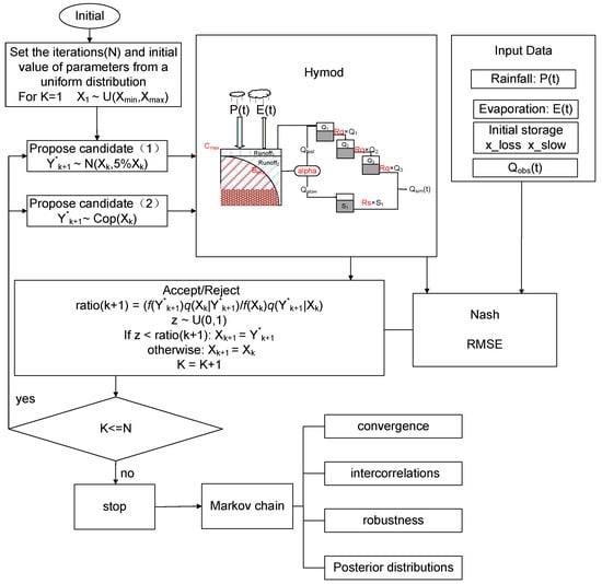
Figure 1. The general framework of the copula-based Bayesian inference approaches.

In this study, the Hymod model is employed as the hydrological modeling core, providing the fundamental hydrologic framework that links model parameters to hydrological responses, particularly streamflow [37]. The model is forced by precipitation and evapotranspiration inputs, while internal soil moisture states govern runoff generation and routing processes. Based on the hydrologic protocol, posterior distributions of parameters are inferred using two MCMC algorithms: the conventional MH algorithm, and the proposed CopMH algorithm. The convergence of the MCMC chains is assessed using Heidelberger and Welch’s convergence diagnostic with the help of the coda package in R. The performance of CopMH is evaluated in comparison with the MH algorithm for identifying the five parameters of the Hymod. The convergence and robustness of proposed methods, as well as intercorrelations among the five Hymod parameters, will be analyzed. In addition, a benchmark optimization algorithm, the Shuffled Complex Evolution (SCE) algorithm, is employed to further assess and compare the simulation accuracy of the proposed CopMH algorithm.

2.1. Bayesian Inference

According to the Bayes equation [38], the posterior distribution $p\left({\theta }_H|Q_{obs}\right)$ of the parameter set ${\theta }_H$ is derived from the prior distribution $p\left({\theta }_H\right)$ conditioned on observed data $Q_{obs}$ as follows:

$$p({\theta }_H|Q_{obs})= {\displaystyle \frac{p({\theta }_H)p(Q_{obs}|{\theta }_H)}{p(Q_{obs})}}$$

(1)

where $p({\theta }_H)$ is the prior distribution of hydrological model parameters, and $L\left({\theta }_H\right|Q_{obs})\equiv p(Q_{obs}\left|{\theta }_H\right)$ denotes the likelihood function, with residual error as follows$: {\epsilon }_i=Q_{obs,i}-Q_{sim,i}$. The prior distribution $p\left({\theta }_H\right)$ explains the information about hydrological model parameter set ${\theta }_H$, before any data are collected. The likelihood function $L\left({\theta }_H |Q_{obs}\right)$ is used to summarize the residual errors between the model simulations and corresponding observations. In this study, the residual errors ${\epsilon }_i$ are assumed to be independent and identically normally distributed with zero mean and constant variance ${\mathsf{\sigma }}_{\epsilon }^2$. The likelihood is constructed under the Gaussian residual error assumption, as described below:

$$L({\theta }_H|Q_{obs},{\sigma }_{\epsilon }^2)={\displaystyle \prod _{i=1}^n\frac{1}{\sqrt{2\pi {\sigma }_{\epsilon }^2}}\exp \left[-\frac{{(Q_{obs}-Q_{sim})}^2}{2{\sigma }_{\epsilon }^2}\right]}$$

(2)

The essence of the parameter estimation problem in the Bayesian filtering framework is to construct the posterior probability density functions of parameters on all previous observations (X_1:K) and current proposed candidate Y*_k+1 [39].

2.2. Metropolis–Hastings Algorithm

The basis of MCMC simulation is a Markov chain that generates a random walk through the search space and successively visits solutions with stable frequencies stemming from a stationary distribution f. The earliest MCMC approach is the Metropolis algorithm introduced by Metropolis et al. (1953) [25]. Then, Hastings [24] introduced a general form of the MCMC algorithm, namely the Metropolis–Hastings algorithm (MH algorithm). To generate a Markov chain (X_k | k = 0, 1, 2, …, n) with stable frequencies stemming from a stationary distribution, the MH algorithm determines trial moves from the current state X_k to a new state X_k+1. In the MH algorithm, all the proposed candidates Y^*_k+1 were generated by transition density $\mathrm{q}(.|X_k)$. The transition density is more flexible. No matter what form of the proposed distribution is selected, the MH algorithm can tend to an equilibrium distribution. But it is more important to choose the transition density, as the convergence speed can be accelerated with a well-selected transition density.

A very popular choice for the transition density $q(·|X_k)$ is the normal distribution $\mathrm{N}(X_k,{\mathsf{\sigma }}_k^2)$, with a mean of $X_k$ and fixed variance of ${\mathsf{\sigma }}_k^2$. In our study, ${\mathsf{\sigma }}_k^2$ is selected as 5%${\ast X}_k$. The proposed candidate Y^*_k+1 is then accepted or rejected according to $ratio\left(k+1\right)$, which was calculated as follows:

$$ratio(k+1)={\displaystyle \frac{f(Y_{k+1}^{*})q(X_k|Y_{k+1}^{*})}{f(X_k)q(Y_{k+1}^{*}|X_k)}}$$

(3)

where $f(·)$ is the target distribution of the Markov chain. If runif (1) <ratio(k + 1), the proposed candidate Y^*_k+1 is accepted, and X_k+1 = Y^*_k+1; otherwise, the proposed candidate Y^*_k+1 is rejected, and X_k+1 = X_k. Target distribution $f(·)$ is the posterior probability density functions of parameters in our parametric uncertainty analysis problem. According to the Bayes equation and Equations (1)–(3), Equation (4) can be converted to Equation (4) as follows:

$$\begin{array}{ll}ratio(k+1)& ={\displaystyle \frac{p(Y_{k+1}^{*}|Q_{sim,k+1}^{*},Q_{obs})q(X_k|Y_{k+1}^{*})}{p(X_k|Q_{sim,k},Q_{obs})q(Y_{k+1}^{*}|X_k)}}\\ & ={\displaystyle \frac{p({\epsilon }_{k+1}^{*}|Y_{k+1}^{*},Q_{sim,k+1}^{*},Q_{obs})p(Y_{k+1}^{*})q(X_k|Y_{k+1}^{*})}{p({\epsilon }_k|X_k,Q_{sim,k},Q_{obs})p(X_k)q(Y_{k+1}^{*}|X_k)}}\end{array}$$

(4)

In this research, all of the prior distributions $p(·)$ are assumed to be uniform distributions, and if the transition density $q(·|·)$ in the MH algorithm is assumed to be a normal distribution with symmetric dependencies, then

$${\displaystyle \frac{p(Y_{k+1}^{*})q(X_k|Y_{k+1}^{*})}{p(X_k)q(Y_{k+1}^{*}|X_k)}}=1$$

(5)

Therefore, Equation (5) can translate into Equation (6) equivalently.

$$ratio(k+1)={\displaystyle \frac{{\displaystyle \prod _{i=1}^n\frac{1}{\sqrt{2\pi {\sigma }_{{\epsilon }_{k+1}^{*}}^2}}\exp \left[-\frac{{({\epsilon }_{{k+1}_i}^{*})}^2}{2{\sigma }_{{\epsilon }_{k+1}^{*}}^2}\right]}}{{\displaystyle \prod _{i=1}^n\frac{1}{\sqrt{2\pi {\sigma }_{{\epsilon }_k}^2}}\exp \left[-\frac{{({\epsilon }_{k_i})}^2}{2{\sigma }_{{\epsilon }_k}^2}\right]}}}$$

(6)

The proposal distribution $q(·|·)$ plays a crucial role in the performance of the MH algorithm, as it directly governs the size and direction of proposed moves. Algorithmic efficiency is determined by an appropriate balance between acceptance and effective exploration of the parameter space. An excessively high acceptance rate usually indicates that proposed moves are too small, which leads to slow exploration and highly correlated samples, whereas an excessively low acceptance rate implies that most proposals are rejected, resulting in poor mixing. In standard MH implementations, Gaussian proposal distributions are widely adopted. However, such proposal distributions often perform poorly in high-dimensional parameter spaces, as they tend to generate small moves and frequent repeated samples. Moreover, the standard MH algorithm typically ignores the intrinsic dependencies among hydrological parameters. Strong parameter dependencies combined with high-dimensional sampling spaces force MH algorithms to adopt overly conservative update schemes, further reducing sampling efficiency. Therefore, to perform efficient inference in hydrological models, it is essential to explicitly account for parameter dependence when designing proposal distributions, motivating the development of alternative, dependence-aware proposals within the MH framework.

2.3. Modeling Multiple Dependence Through Copulas

A d-dimensional copula is the function mapping from [0, 1]^d to [0, 1]. Consider random vectors X₁, X₂, …, X_d with the marginal distributions denoted as F1, F2, …, Fd and the joint distribution denoted as F(x₁, x₂, …, x_d). According to Sklar’s theorem, for all x∈R, R∈(−∞, +∞), there exists a copula C, and the relationship between joint distribution F(x₁, x₂, …, x_d) and copula function C can be expressed as follows [35]:

$$F\left(x_1,x_2,\cdots x_d\right)=C\left[F_1\left(x_1\right),F_2\left(x_2\right),\cdots ,F_d\left(x_d\right)\right]=C\left(u_1,u_2,\cdots ,u_d\right)$$

(7)

where C (.) is a copula function; $F_i$ is a continuous function; and $u_i=F_i\left(x_i\right)$ and $u_i~\mathrm{U}\left(\mathrm{0,1}\right)$ for i = 1, 2, …, d. If $f_i\left(x_i\right)$ is the probability density corresponding to ${F_i(x}_i)$ and c(.) is the density function corresponding to copula C(.), then $c\left(u_1,u_2,\dots ,u_d\right)$ and $f\left(x_1,x_2,\dots ,x_d\right)$ can be described as follows:

$$c\left(u_1,u_2,\cdots ,u_{\mathrm{d}}\right)={\displaystyle \frac{{\partial }^{d}C\left(u_1,u_2,\cdots ,u_{\mathrm{d}}\right)}{\partial u_1\partial u_2\cdots \partial u_d}}$$

(8)

$$f\left(x_1,x_2,\cdots ,x_{\mathrm{d}}\right)=c\left(u_1,u_2,\cdots ,u_{\mathrm{d}}\right){\displaystyle \prod _{i=1}^d{f}_i\left(x_i\right)}$$

(9)

As modeling of the marginal distributions can be conveniently separated from the dependence modeling, there is flexibility in selecting both marginal and dependent models of copulas [1,39]. More details on the theoretical background and properties of various copula families can be found in [36,40]. A number of bivariate copula functions have been developed, mainly including the Archimedean, elliptical, and extreme value copulas [33]. However, for random variables larger than three, there exist only a limited number of available copula families that allow for efficient sample generation and the standard multivariate copulas may not model their interdependence [39]. With the development of the pair-copula approach, multivariate copulas have recently been greatly extended through d(d − 1)/2 bivariate copulas [41]. Among the possible pair-copula constructions, the vine copulas including the canonical vine (C-vine) and D-vine were used widely as decomposition structures. The structures of the C-vine and D-vine for five random variables are shown in Figure 2.

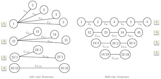
Figure 2. The structures of the C-vine and D-vine for five random variables.

For C-vine,

$$f_{12345}=c_{12}{c}_{13}{c}_{14}{c}_{15}{c}_{23|1}{c}_{24|1}{c}_{25|1}{c}_{34|12}{c}_{35|12}{c}_{45|123}{\displaystyle \prod _{i=1}^5{f}_i}$$

(10)

For D-vine,

$$f_{12345}=c_{12}{c}_{23}{c}_{34}{c}_{45}{c}_{13|2}{c}_{24|3}{c}_{35|4}{c}_{14|23}{c}_{25|34}{c}_{15|234}{\displaystyle \prod _{i=1}^5{f}_i}$$

(11)

The pair-copula constructions decompose a multivariate probability density into bivariate copulas, with each pair-copula chosen independently from the others, which allows for enormous flexibility in dependence modeling [39].

2.4. MH and CopMH Algorithms

In the CopMH algorithm, the dependence structure of model parameters is quantified through copulas, and model parameters are then sampled based on the obtained copula functions. The CopMH algorithm improves upon the standard MH algorithm through generating new proposal candidates ${\mathit{Y}}_{k+1}^{\mathrm{*}}$ based on the joint probability function of the parameters derived from the vine copula, and by applying a joint parameter update scheme in each proposal distribution. Essentially, CopMH constitutes a dependence-sampling algorithm with a proposal distribution that closely approximates the target distribution, resulting in higher sampling efficiency. The main difference between MH and CopMH lies in the transition densities $q\left(·|{\mathit{X}}_k\right)$ of the proposed candidates ${\mathit{Y}}_{k+1}^{\mathrm{*}}$. In detail, the transition density $q_{MH}(·|{\mathit{X}}_k)$ is a normal distribution $N({\mathit{X}}_k,{ \sigma }_k^2)$ in MH, whereas the transition density $q_{CopMH}(·|{\mathit{X}}_k)$ is a joint probability function obtained from the vine copula in CopMH. In our implementation, the Gaussian copula-based proposals are designed to preserve symmetry in the marginal jumps of the parameters. Therefore, the standard Metropolis acceptance criterion can be applied. However, we note that if an asymmetric proposal distribution were used, the MH framework would be necessary to correctly account for the asymmetry in the acceptance probability, ensuring proper convergence of the Markov chain.

In addition, it is important to note that the computational efficiency and stability of the CopMH algorithm depend on the dimensionality of the database. Higher-dimensional parameter spaces increase the computational burden of fitting the vine copula and require more samples to achieve convergence, while finer temporal resolution enlarges the dataset and extends computation time. A trade-off between computational cost and solution fidelity can be managed by selecting appropriate parameter subsets or applying temporal aggregation when dealing with very large or high-resolution datasets.

The detailed procedure is presented below, while Algorithm S1 in the Supplementary Material provides concise descriptions and pseudocode for the MH and CopMH algorithms. The number of iterations (N) and the initial values of the parameters are set by sampling from their corresponding uniform distributions [4]. Here, ${\mathit{X}}_1$ denotes the initial parameter vector, and $x_{j,min}$ and $x_{j,max}$ denote the predefined lower and upper bounds of each parameter $x_j$, respectively.

• Generate an initial Markov chain. At any step K + 1, the model parameters X_k+1 for the current step can be forecasted based on the prior parameters X_k in step K and the simulated observations Q_sim in the current step. The simulated observations $Q_{sim}$ are obtained through Hymod with model parameters X_k+1. An initial Markov chain $x_{i,j}$ i = 1, …, 1000; $j=\mathrm{1,2},\mathrm{3,4},5$ were generated.
• Uniformization: Based on initial Markov chain $x_j$, the marginal distributions of each parameter are assumed to be normally distributed with mean $\overline{x_j}$ and variance ${\mathsf{\sigma }}_j$. $\overline{x_j}$ and ${\mathsf{\sigma }}_j$ are the mean value and variance value of the prior 1000 prerun samples. Depending on the cumulative probability density function of every Markov chain, each prerun sample $x_{i,j}$ can be transformed to $\mathrm{n}\mathrm{o}\mathrm{r}\mathrm{m}\_x_{i,j}$ in the range [0, 1] using the “pnorm” function in R.
• Fitting the D-vine copula model. Using $\mathrm{n}\mathrm{o}\mathrm{r}\mathrm{m}\_x_{i,j}$, we fit an η-parameterized D-vine copula density, assuming all of the D-vine pair-copula families were Frank copulas. The pair-copula parameters of 5-dimensional D-vine copula models were sequentially estimated using the “CDVineSeqEst” function in “CDVine Package”.
• Generate proposed candidate $Y_{k+1}^{*}$ according to the D-vine copula model. A $1\times 5$ matrix of data y_copula was simulated from the above D-vine copula model using the “CDVineSim” function in “CDVine Package”. Then the proposed candidates $Y_{k+1}^{*}$ were generated as a quantile function of the normal distribution based on inversion of pnorm using the “qnorm” function in R.
• Generate proposed candidates for the CopMH algorithm.
  Now, let y₁ be a random MH algorithm proposed candidate of choice, and y₂ be a CopMH algorithm proposed candidate.
• Generation of the Markov chain. Run Hymod with model parameters $y_{k+1}^{*}$, and obtain the simulated observations ${Q^{*}}_{sim}$. Then calculate $\mathrm{r}\mathrm{a}\mathrm{t}\mathrm{i}\mathrm{o}(\mathrm{k}+1)$ according to Equation (7). Loop iterations until K = 20,000.

3. Case Study

3.1. Hydrologic Simulation and Model Calibration and Validation

3.1.1. Hydrologic Simulation

In this study, rainfall–runoff simulation is performed using a simple conceptual model—Hymod—to generate daily streamflows. The general concept of the model is based on the probability distribution of soil moisture modeling proposed by Moore [42]. Water storage dynamics are based on mass balance principles with inflow from rainfall, losses to evaporation, drainage to groundwater (recharge), and production of direct runoff. In brief, a catchment is represented as consisting of infinitely many points, each defined by a soil moisture capacity C. Soil moisture capacities vary within the catchment as a result of variability in soil texture and depth. A cumulative distribution function (CDF) is used to describe the variability of catchment soil moisture (Equation (13)):

$$F\left(c\right)=1-{\left[1-{\displaystyle \frac{c}{C_{\max }}}\right]}^{B\exp }\hspace{1em}\hspace{1em}0\le c\le C_{\max }$$

(12)

where c is soil moisture capacity, Cmax is the maximum storage capacity, and the exponent Bexp is the degree of spatial variability of storage capacity over the basin. Alpha is introduced to represent how much of the subsurface runoff is routed over the fast (Rq) and slow (Rs) pathway. The descriptions and initial fluctuating ranges of the five parameters are shown in Table 1. Daily input data of precipitation, P (mm/d), and potential evapotranspiration, E (mm/d), are used to drive the conceptual rainfall–runoff model. The five parameters, including Cmax, Bexp, Alpha, Rs, and Rq, cannot be measured directly, but can be obtained through a model calibration process [8]. A schematic representation of the Hymod model is shown in Figure 1. For the sake of brevity, we refer our readers to [42,43] for a comprehensive description of Hymod.

Table 1. The descriptions and initial fluctuating ranges of Hymod parameters.

Parameter	Description	Range	References
Cmax	Maximum soil moisture capacity within the catchment (mm)	[200, 500]	[4,11,12,43]
Bexp	Shape factor that is dependent on the degree of spatial variability in soil moisture capacities	[0.01, 2]
Alpha	Fraction coefficient for distribution of water between slow and quick reservoirs	[0.5, 0.9]
Rq,	Inverse of residence time in quick reservoirs (1/day)	[0.01, 0.2]
Rs,	Inverse of residence time in a slow reservoir (1/day)	[0.3, 0.7]

3.1.2. Model Performance Evaluation

Model calibration is an essential procedure to obtain the optimal parameter values, which match simulated data and observed data as closely as possible. In this study, calibration and validation are performed according to the three algorithms. For the goodness of fit, Nash–Sutcliffe model efficiency (Nash) and the root mean square error (RMSE) are used to assess the predictive power of model results. Nash is commonly used for model evaluations [44,45], because it involves standardization of the residual variance and its expected value does not change with the length of the record or the scale of the runoff. Here, the objective functions adopted can be represented as follows [46,47]:

$$Nash=1-{\displaystyle \frac{{\displaystyle {\sum }_{i=1}^n{\left(Q_{obs,i}-Q_{sim,i}\right)}^2}}{{\displaystyle {\sum }_{i=1}^n{\left(Q_{obs,i}-\overline{Q_{obs}}\right)}^2}}}$$

(13)

The RMSE can be expressed as

$$RMSE=\sqrt{{\displaystyle \frac{{\displaystyle {\sum }_{i=1}^n{\left(Q_{obs,i}-Q_{sim,i}\right)}^2}}{n}}}$$

(14)

where $Q_{sim}$ is the simulated runoff, $Q_{obs}$ is the observed runoff, and $\overline{Q_{obs}}$ is the mean value of the observed runoff. $n$ is the sample size.

3.2. Study Catchment and Data Acquisition

3.2.1. Study Catchment

The developed CopMH approach is applied to address parameter uncertainties and their interactions for the Ruihe River, which is a tributary of Jinghe River located in the middle of the Loess Plateau in China. The catchment area of the Ruihe River is 1670 km² with a main stream length of 119 km, and the elevation varies from 1200 to 2645 m. The average annual temperature represents the spatially varying annual mean temperature across the catchment, ranging from 7.7 °C to 10 °C due to elevation differences. The average annual precipitation is 562 mm, and nearly 60–70% of precipitation occurs between June and September. Evapotranspiration (E) in this study was calculated using the Penman–Monteith method. The Ruihe River plays an important role in mitigating water loss, reducing soil erosion, and protecting the ecosystem of the middle reach of the Jinghe River. Hydrological modeling in this watershed is thus desired, which can help to more accurately describe the hydrological processes and promote water resource management.

3.2.2. Data Acquisition

A series of model inputs is required for Hymod model simulation, including daily evaporation, daily precipitation, and initial water loss. In this study, the data of the Ruihe River watershed in these categories were collected from different sources. The areal daily precipitation (denoted as P) data were interpolated from site precipitation measurements distributed over the catchment, and the areal potential daily evapotranspiration (denoted as E) data were interpolated from the E data at the national meteorological stations as shown in Figure 3a. The daily runoff data of the Ruihe River (from 1981 to 1987) were obtained from Yuanjiaan Hydrometric Station as shown in Figure 3b. The input topography map was collected to derive the flow direction and hydrographic network. DEMs (1:250,000) were obtained from the Data Center for Resources and Environmental Sciences, Chinese Academy of Sciences (RESDC) (http://www.resdc.cn).

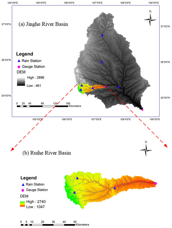
Figure 3. The location of the studied catchments: (a) the Jing River basin and (b) the Ruihe River basin. The blue triangles show the location of national meteorological stations used to generate the potential evapotranspiration and precipitation, and the purple cycles indicate the location of the gauge station.

3.2.3. Data Analysis

In this study, four-year daily discharge observations (1461 samples) were used for parameter calibration. The discrepancy between the observed and simulated discharges was characterized by model residuals, which were assumed to be independently and identically distributed Gaussian variables with zero mean. This assumption enables observational uncertainty to be explicitly incorporated into the likelihood-based inference framework. The Nash values were employed as a performance metric to evaluate model simulations [48,49]. To avoid the influence of initial transients, the first 50 samples were excluded when computing Nash values.

Convergence of the Markov chains was assessed using the Heidelberger and Welch diagnostic to ensure that posterior samples were drawn from a stationary distribution [50,51]. For this purpose, the first 1000 iterations of each chain were discarded as burn-in. The diagnostic is based on the Cramér–von Mises statistic, which tests the null hypothesis that the sampled values originate from a stationary process. The detailed procedure follows Heidelberger and Welch [4] and was implemented using the Output Analysis and Diagnostics for MCMC (CODA) package in R.

To compare the performance of the MH and CopMH algorithms, the marginal posterior probability density functions (PDFs) of the five Hymod parameters were estimated using Gaussian kernel density estimation based on the last 10,000 samples of each Markov chain. Furthermore, to assess the robustness of the proposed method, three algorithms (MH, CopMH, and the benchmark algorithm) were independently repeated 15 times under the same sampling scenario with 20,000 iterations. Boxplots of the five parameters and Nash values, derived from the last 10,000 samples of each Markov chain, are presented to illustrate the variability and stability of parameter estimates across different runs.

4. Results and Discussion

4.1. Convergence of Algorithm

In this study, the prior densities for five parameters of Hymod are assumed to cover a wide range to represent vague prior knowledge and are sampled uniformly from their prespecified intervals, as presented in Table 1. Figure 4 illustrates path diagrams of the parameters estimated using the MH and CopMH algorithms, with each Markov chain containing 20,000 iterations for each parameter. The results indicate that all five Hymod parameters are well identified after certain a number of iterations, even under wide prior distributions. Markov chains with more than 10,000 iterations appear sufficient to characterize the posterior parameter distributions with relatively limited ranges. As shown in Figure 4, the Markov chains obtained using the MH algorithm exhibit unstable behavior with wide fluctuations (e.g., Alpha, Rq). In contrast, the proposed CopMH algorithm leads to parameter evolution within clearly narrow fluctuation ranges, suggesting that copula-based proposals can substantially improve sampling efficiency and accuracy.

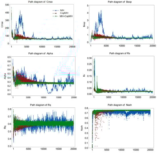
Figure 4. Path diagram of the parameters estimated using MH (blue curves), CopMH (red curves), and their hybrid approach (green curves), with one Markov chain containing 20,000 iterations for each parameter.

Table 2 presents the significance level (p-value) of Markov chains containing 1000–20,000 iterations. A p-value larger than 0.05 indicates that the null hypothesis is accepted, suggesting convergence of the chain. From Table 2, all p-values—except Rq obtained by MH and Rq obtained by CopMH—exceed 0.05, demonstrating the convergence of the proposed method. Moreover, examination of the parameter trace plots shows that CopMH converges faster than MH, indicating improved efficiency achieved by introducing the copula proposal distribution.

Table 2. The significance level (p-value) of Markov chains containing 10,000–20,000 iterations tested using the Cramer–von Mises statistic.

	Cmax	Bexp	Alpha	Rs	Rq
MH	0.333	0.190	0.270	0.558	0.009
CopMH	0.896	0.843	0.586	0.678	0.492

Compared with the original MH algorithm, significant improvements in the Nash value are also observed in the CopMH algorithm, as shown in Figure 4. In detail, after 10,000 iterations, Nash values of simulation results obtained by the MH algorithm ranged from 0.6 to 0.75, and few Nash values were less than 0.6. Meanwhile, the Nash values were basically stable around 0.76 (Figure 4) for CopMH under the same iterations. The results indicated the simulation accuracy is greatly improved and the simulation error caused by parameters is reduced through introducing the copula.

4.2. Intercorrelation Analysis Between Parameters

In hydrological models, multiple parameters generally have interactive effects on model outputs [20], which thus depend on the values of the interrelated parameters [10]. Similarly, such interrelationships among parameters exist in the parameter iteration process.

Figure 5 presents the correlogram of parameter intercorrelations of Hymod measured through Pearson correlations with MH and CopMH. As shown in Figure 5, the interrelationships among different pairs of parameters are varied under the two algorithms. Taking MH as an example, Cmax-Bexp pairs showed a strong positive correlation while Alpha-Rq pairs exhibited a significant negative correlation structure. At the same time, Rs-Rq and Alpha-Rs showed a weak positive correlation and Bexp-Rs showed a weak negative correlation. The results indicate that the interdependence structures of the five parameters in Hymod are ubiquitous but not always significant. Previous studies have shown that the correlations between Hymod model parameters are related to precipitation, potential evapotranspiration, and streamflow discharge, and such correlations mainly showed nonlinear features. The results also reflected that the introduction of copulas in multivariate hydrologic modeling is meaningful and necessary, which can reflect the interdependent structure between parameters.

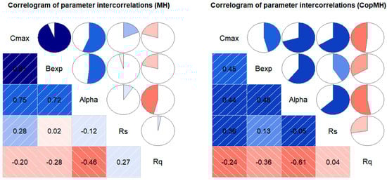
Figure 5. Correlogram of Pearson correlation coefficients among Hymod parameters estimated by the MH and CopMH algorithms. Shaded cells in the lower triangle indicate correlation magnitude (blue: positive; red: negative), while pie charts in the upper triangle represent correlation strength. Numerical values are shown within each cell.

4.3. Bayesian Inference of Model Parameters

Figure 6 presents the marginal posterior probability density functions (PDFs) of the five Hymod parameters estimated using the MH and CopMH algorithms. From the results, posterior distributions of the five parameters in this study differ in a range different from their prior distributions. Take the MH algorithm as an example; the ranges of posterior distributions are [45.80, 104.61] for Cmax, [0.34, 1.15] for Bexp, [0.016, 0.531] for Alpha, [0.009, 0.054] for Rs, and [0.44, 0.79] for Rq (Figure 6a). The latter is approximately normally distributed with a relative symmetric distribution, while significant skewness is present in the posterior distributions of Cmax, Bexp, Alpha, and Rs. Compared with the MH algorithm, significant narrow convergence ranges are observed through the CopMH algorithm, specifically [61.16, 63.08] for Cmax, [0.56, 0.64] for Bexp, [0.258, 0.301] for Alpha, [0.020,0.025] for Rs, and [0.59,0.62] for Rq. Moreover, the posterior distributions of the five parameters estimated using the CopMH algorithm are approximately normal distributions with a relatively symmetric distribution, indicating that the posterior distributions of parameters are well defined by the CopMH algorithm. It is also found that the three algorithms can obtain almost identical means and standard variances for each parameter (Table 3), which indicates the estimation accuracy of the CopMH algorithm.

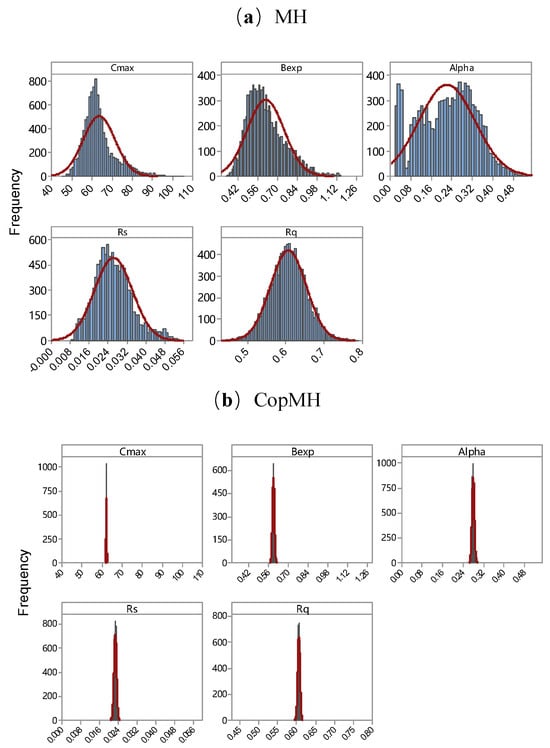
Figure 6. Posterior distributions of the five Hymod parameters obtained by the MH (a) and CopMH (b) algorithms. Histograms indicate sampled parameter values, and the overlaid lines represent Gaussian kernel-estimated density curves.

Table 3. Summary statistics of the posterior PDFs of the five Hymod parameters obtained using the MH and CopMH algorithms. The variance reduction indicates the relative decrease in posterior uncertainty achieved by CopMH.

Parameter	MH		CopMH		Variance Reduction (%)
	Mean	Sd	Mean	Sd
Cmax	63.68	7.90	62.14	0.15	99.96
Bexp	0.616	0.131	0.596	0.007	99.71
Alpha	0.219	0.109	0.279	0.005	99.79
Rs	0.0264	0.0081	0.0228	0.0006	99.45
Rq	0.6072	0.0473	0.6065	0.0031	99.57

4.4. Robustness of Algorithm

Figure 7 presents boxplots of the five parameters and Nash values of each Markov chain, obtained from 15 independent runs of the two algorithms. The performance of MH exhibits significant variation with a relatively wide range especially for Alpha, Rs, Rq, and Nash, as presented in Figure 7. Meanwhile, the distributions converged to a stationary value with a markedly narrow range through CopMH and HCopMH. For instance, as presented in Figure 7, the generated Rs values vary from 0.006 to 0.061 for MH while the ranges are only 0.021–0.032 and 0.019–0.034 for CopMH and HCopMH across the 15 independent replicates. For the probabilistic forecasts obtained from MH, the associated Nash values range from 0.63 to 0.76, while Nash values obtained from CopMH and HCopMH are approximately larger than 0.74 for all replicates. This indicates that the performances of CopMH and HCopMH are generally quite reliable with limited fluctuating ranges for all five parameters and the Nash indicator. By comparison, HCopMH exhibits the strongest robustness.

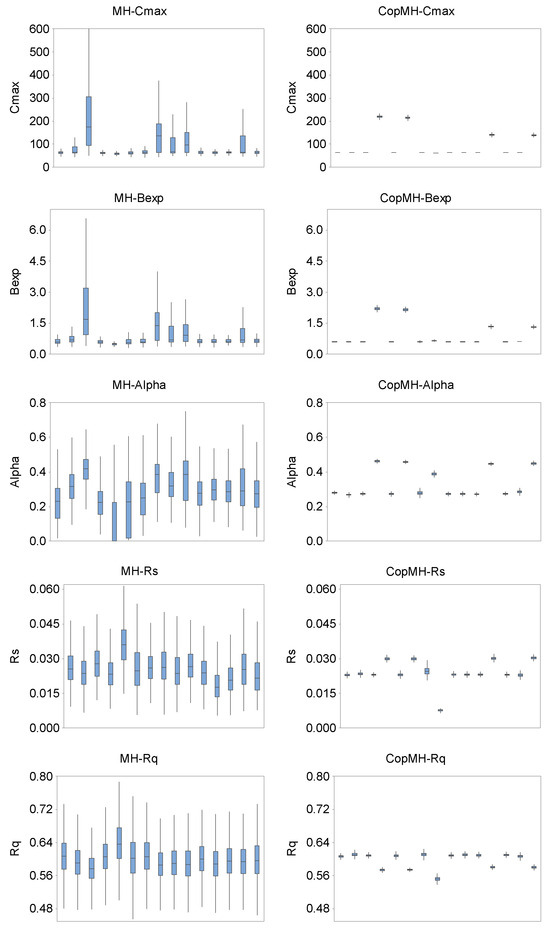
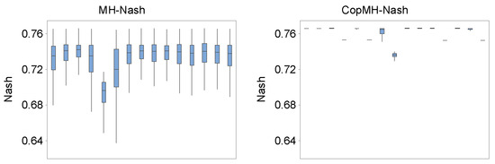
Figure 7. Boxplots of five parameters and Nash value of the last 10,000 samples in the Markov chains, for 15 independent runs, obtained by MH (the first column) and CopMH (the second column).

4.5. Calibration and Verification of the Hydrologic Model

The uncertainty in model parameters can be propagated into hydrological model simulation uncertainty and affect model calibration [10,47]. In this study, to investigate the transmission of uncertainty, hydrological simulations with Hymod were performed over a calibration period of 1461 continuous daily records (1981–1984), and then validated using 1095 daily streamflow observations (1985–1987). Model calibration and validation were conducted using the daily observation data at Yuanjiaan Hydrometric Station. The 95% confidence intervals of daily discharge of the posterior PDFs are presented in Figure 8.

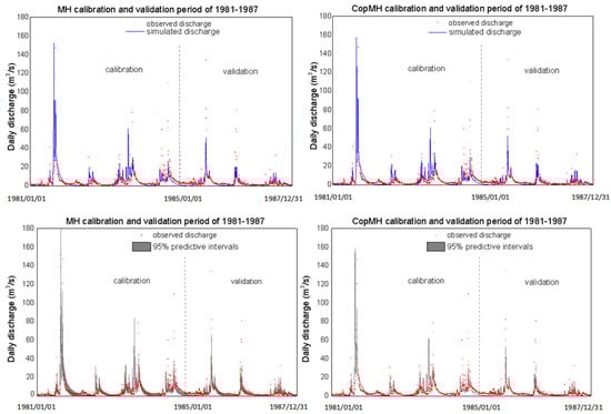
Figure 8. Comparison between predictions from different schemes and real observations: the red points indicate the observed values while the blue line shows predictive means of daily streamflow (Q: m³/s) during 1981–1987 at Yuanjiaan station at Ruihe River basin. The gray belt exhibits the 95% predictive intervals consisting of the 2.5% and 97.5% quantile values.

The performance of the simulation was evaluated using the Nash–Sutcliffe efficiency (Nash) and RMSE. The 2.5%, mean, and 97.5% values of Nash and RMSE for the calibration and verification periods are presented in Table 4 for different algorithms. Most of the Nash values are larger than 0.76 in the calibration period and larger than 0.64 in the verification period, indicating that Hymod provides a reasonably good simulation of the Ruihe River watershed. Compared with MH, CopMH performs better, achieving higher Nash values and lower RMSE values in both calibration and verification periods. This improvement is attributed to the consideration of parameter correlations through the copula, which enhances the accuracy of the hydrological model results. It should be noted that, as observed in Figure 8, the uncertainty bounds estimated by CopMH are slightly narrower than those of MH. This is because CopMH improves sampling efficiency by capturing the dependence structure among parameters, leading to reduced variability in the posterior samples. While the uncertainty intervals are somewhat narrower, the parameter estimates remain unbiased and the overall posterior distributions still provide a reliable quantification of hydrological uncertainty.

Table 4. Performance comparison of MH, CopMH, and HCopMH on Hymod model at Ruihe River.

		Nash			RMSE
		2.5%	97.5%	mean	2.5%	97.5%	mean
MH	calibration	0.673	0.663	0.761	6.946	7.051	5.937
	validation	0.432	0697.	0.635	5.834	4.261	4.678
CopMH	calibration	0.766	0.765	0.766	5.871	5.884	5.872
	validation	0.637	0.649	0.642	4.665	4.584	4.628

Moreover, to compare and analyze simulation accuracy of the developed algorithm, a benchmark optimization algorithm—the SCEUA algorithm—is also utilized in our study. The five parameters are 209.1, 1.978, 0.50, 0.0287, and 0.568, respectively, estimated through SCEUA. The predictions of daily discharge calculated by SCEUA are presented in Figure 9. And the corresponding Nash values of calibration and validation are 0.75 and 0.673. RMSE values of calibration and validation obtained are 6.041 and 4.427. It is found that, in all the three sample evolution schemes, some parameters may not converge to their true values (e.g., Cmax, Bexp, and Alpha), which are obtained through SCEUA, while the Nash values are equal to or higher than 0.75, which are obtained through SCEUA. The results show the presence of equifinality during the modeling of Hymod in Jinghe River, which is the phenomenon whereby multiple parameter sets produce an equally good or bad simulation performance. Previous studies have reported that the equifinality problem has been universally found in hydrological models [20,27]. Li et al. provide a comprehensive discussion about the sources of equifinality in a distributed conceptual hydrological model and find that overparameterization, systematic errors of input data, and too few constraint conditions are the sources of equifinality in the model [45]. Her & Chaubey also demonstrated that equifinality is responsive to the numbers of observations and calibration parameters and substantial equifinality did not necessarily mean bad model performance nor large uncertainty in the model outputs and parameters [45].

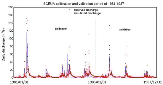
Figure 9. Prediction from SCEUA and real observations: the red points indicate the observed values while the blue line shows predictive means of daily streamflow (Q: m³/s) during 1981–1987 at Yuanjiaan station at Ruihe River basin.

5. Conclusions

This study proposes a copula-based Metropolis–Hastings (CopMH) algorithm to enhance Bayesian parameter inference in hydrological models by explicitly accounting for interdependence among model parameters. By embedding copula functions into the MH sampling framework, the proposed approach enables joint sampling from dependent parameter spaces and improves sampling efficiency. Application to the Hymod model in the Ruihe River watershed demonstrates that CopMH achieves faster convergence, substantially reduced posterior uncertainty, and enhanced robustness compared with the conventional MH algorithm, while maintaining comparable or improved simulation performance in terms of the Nash–Sutcliffe efficiency and RMSE. These results confirm that parameter interdependence is ubiquitous in hydrological models and that explicitly modeling such dependence is both meaningful and beneficial for uncertainty quantification.

Despite these advantages, the CopMH approach is subject to several limitations. Its performance depends on the choice of copula function, and the computational cost may increase for higher-dimensional parameter spaces. Future research will focus on adaptive or data-driven copula selection strategies, extension to more complex and distributed hydrological models, and broader evaluation across different climatic and hydrological conditions.

References

- Fan, Y.R.; Huang, G.H.; Baetz, B.W.; Li, Y.P.; Huang, K.; Li, Z.; Chen, X.; Xiong, L.H. Parameter uncertainty and temporal dynamics of sensitivity for hydrologic models: A hybrid sequential data assimilation and probabilistic collocation method. Environ. Model. Softw. 2016, 86, 30–49. [Google Scholar] [CrossRef]
- Solanki, H.; Vegad, U.; Kushwaha, A.; Mishra, V. Improving streamflow prediction using multiple hydrological models and machine learning methods. Water Resour. Res. 2025, 61, e2024WR038192. [Google Scholar] [CrossRef]
- Wang, F.; Huang, G.H.; Fan, Y.; Li, Y.P. Development of clustered polynomial chaos expansion model for stochastic hydrological prediction. J. Hydrol. 2021, 595, 126022. [Google Scholar] [CrossRef]
- Heidelberger, P.; Welch, P.D. Simulation Run Length Control in the Presence of an Initial Transient. Oper. Res. 1983, 31, 1109–1144. [Google Scholar] [CrossRef]
- Moradkhani, H.; Hsu, K.L.; Gupta, H.; Sorooshian, S. Uncertainty assessment of hydrologic model states and parameters: Sequential data assimilation using the particle filter. Water Resour. Res. 2005, 41, 237–246. [Google Scholar] [CrossRef]
- Nash, J.E.; Sutcliffe, J.V. River flow forecasting through conceptual models part I—A discussion of principles. J. Hydrol. 1970, 10, 282–290. [Google Scholar] [CrossRef]
- Yuan, Q.S.; Wang, P.F.; Wang, C.; Chen, J.; Wang, X.; Liu, S. Metal(loid) partitioning and transport in the Jinsha River, China: From upper natural reaches to lower cascade reservoirs-regulated reaches. J. Environ. Inform. 2024, 44, 126–139. [Google Scholar] [CrossRef]
- Fan, Y.R.; Huang, G.H.; Baetz, B.W.; Li, Y.P.; Huang, K. Development of a copula-based particle filter (CopPF) approach for hydrologic data assimilation under consideration of parameter interdependence. Water Resour. Res. 2017, 53, 4850–4875. [Google Scholar] [CrossRef]
- Vrugt, J.A.; Diks, C.G.H.; Gupta, H.V.; Bouten, W.; Verstraten, J.M. Improved Treatment of Uncertainty in Hydrologic Modeling: Combining the Strengths of Global Optimization and Data Assimilation; Pontifical Institute of Mediaeval Studies: Toronto, ON, Canada, 2005; pp. 407–412. [Google Scholar]
- Liu, Y.R.; Li, Y.P.; Huang, G.H.; Zhang, J.L.; Fan, Y.R. A Bayesian-based multilevel factorial analysis method for analyzing parameter uncertainty of hydrological model. J. Hydrol. 2017, 553, 750–762. [Google Scholar] [CrossRef]
- Bastola, S. The regionalization of a parameter of HYMOD, a conceptual hydrological model, using data from across the globe. HydroResearch 2022, 5, 13–21. [Google Scholar] [CrossRef]
- Zhang, K.; Wu, H.; Zhang, J.; Wu, S. Efficient Markov Chain Monte Carlo sampling for Bayesian inverse problems with covariance matrix adaptation. J. Hydrol. 2025, 663, 134235. [Google Scholar] [CrossRef]
- Abbas, S.A.; Bailey, R.T.; White, J.T.; Arnold, J.G.; White, M.J.; Čerkasova, N.; Gao, J. A framework for parameter estimation, sensitivity analysis, and uncertainty analysis for holistic hydrologic modeling using SWAT+. Hydrol. Earth Syst. Sci. 2024, 28, 21–48. [Google Scholar] [CrossRef]
- Gupta, A.; Govindaraju, R.S. Uncertainty quantification in watershed hydrology: Which method to use? J. Hydrol. 2023, 616, 128749. [Google Scholar] [CrossRef]
- Wang, G.Q.; Zhang, Q.Z.; Wang, P.Z.; Xue, B.L.; Gao, Z.Y.; Peng, Y.B. Water Quality Prediction Based on an Innovated Physical and Data Driving Hybrid Model at Basin Scale. J. Environ. Inform. 2024, 43, 141. [Google Scholar]
- Brooks, S. Markov chain Monte Carlo method and its application. J. R. Stat. Soc. 1998, 47, 69–100. [Google Scholar] [CrossRef]
- Li, L.; Xia, J.; Xu, C.Y.; Chu, J.J.; Wang, R.; Cluckie, I.D.; Chen, Y.; Babovic, V.; Konikow, L.; Mynett, A. Analyse the sources of equifinality in hydrological model using GLUE methodology, paper presented at Hydroinformatics in Hydrology, Hydrogeology and Water Resources. In Proceedings of the of Symposium Js.4 at the Joint Iahs & Iah Convention, Hyderabad, India, 6–12 September 2009. [Google Scholar]
- Wang, F.; Huang, G.H.; Fan, Y.; Li, Y.P. Development of a disaggregated multi-level factorial hydrologic data assimilation model. J. Hydrol. 2022, 610, 127802. [Google Scholar] [CrossRef]
- Kavetski, D.; Kuczera, G.; Franks, S.W. Bayesian analysis of input uncertainty in hydrological modeling: 1. Theory. Water Resour. Res. 2006, 42, W03407. [Google Scholar] [CrossRef]
- Mara, T.A.; Fajraoui, N.; Younes, A.; Delay, F. Inversion and uncertainty of highly parameterized models in a Bayesian framework by sampling the maximal conditional posterior distribution of parameters. Adv. Water Resour. 2015, 76, 1–10. [Google Scholar] [CrossRef]
- Gregory, P.C. Bayesian exoplanet tests of a new method for MCMC sampling in highly correlated model parameter spaces. Mon. Not. R. Astron. Soc. 2018, 410, 94–110. [Google Scholar] [CrossRef]
- Demirel, M.C.; Koch, J.; Rakovec, O.; Kumar, R.; Mai, J.; Müller, S.; Thober, S.; Samaniego, L.; Stisen, S. Tradeoffs between temporal and spatial pattern calibration and their impacts on robustness and transferability of hydrologic model parameters to ungauged basins. Water Resour. Res. 2024, 60, e2022WR034193. [Google Scholar] [CrossRef]
- De León Pérez, D.; Salazar-Galán, S.; Francés, F. Beyond Deterministic Forecasts: A Scoping Review of Probabilistic Uncertainty Quantification in Short-to-Seasonal Hydrological Prediction. Water 2025, 17, 2932. [Google Scholar] [CrossRef]
- Hastings, W.K. Monte Carlo sampling methods using Markov chains and their applications. Biometrika 1970, 57, 97–109. [Google Scholar] [CrossRef]
- Metropolis, N.; Rosenbluth, A.; Rosenbluth, M.; Teller, A.; Teller, E. Equation of state calculations by fast computing machines. J. Chem. Phys. 1953, 21, 1087–1096. [Google Scholar] [CrossRef]
- Deng, C.; Liu, P.; Wang, D.; Wang, W. Temporal variation and scaling of parameters for a monthly hydrologic model. J. Hydrol. 2018, 558, 290–300. [Google Scholar] [CrossRef]
- Vrugt, J.A.; Gupta, H.V.; Bouten, W.; Sorooshian, S. A Shuffled Complex Evolution Metropolis algorithm for optimization and uncertainty assessment of hydrologic model parameters. Water Resour. Res. 2003, 39, 113–117. [Google Scholar] [CrossRef]
- Zhang, J.; Li, Y.; Huang, G.; Chen, X.; Bao, A. Assessment of parameter uncertainty in hydrological model using a Markov-Chain-Monte-Carlo-based multilevel-factorial-analysis method. J. Hydrol. 2016, 538, 471–486. [Google Scholar] [CrossRef]
- Zhang, J.; Lin, G.; Li, W.; Wu, L.; Zeng, L. An Iterative Local Updating Ensemble Smoother for Estimation and Uncertainty Assessment of Hydrologic Model Parameters With Multimodal Distributions. Water Resour. Res. 2018, 54, 1716–1733. [Google Scholar] [CrossRef]
- Mattingly, J.C.; Pillai, N.S.; Stuart, A.M. Diffusion limits of the random walk Metropolis algorithm in high dimensions. Ann. Appl. Probab. 2010, 22, 881–930. [Google Scholar] [CrossRef]
- Vrugt, J.A. Markov chain Monte Carlo simulation using the DREAM software package: Theory, concepts, and MATLAB implementation. Environ. Model. Softw. 2016, 75, 273–316. [Google Scholar] [CrossRef]
- Haario, H.; Saksman, E.; Tamminen, J. An Adaptive Metropolis Algorithm. Bernoulli 2001, 7, 223. [Google Scholar] [CrossRef]
- Holden, L.; Hauge, R.; Holden, M. Adaptive Independent Metropolis-Hastings. Ann. Appl. Probab. 2009, 19, 395–413. [Google Scholar] [CrossRef]
- Sklar, M. Fonctions de repartition a N dimensions et leurs marges. Annales de l’ISUP 1959, 8, 223–231. [Google Scholar]
- Lei, X.H.; Tan, Q.F.; Wang, X.; Wang, H.; Wen, X.; Wang, C.; Zhang, J.W. Stochastic optimal operation of reservoirs based on copula functions. J. Hydrol. 2017, 557, 265–275. [Google Scholar] [CrossRef]
- Favre, A.C.; Adlouni, S.E.; Perreault, L.; Thiémonge, N.; Bobée, B. Multivariate hydrological frequency analysis using copulas. Water Resour. Res. 2004, 40, 290–294. [Google Scholar] [CrossRef]
- Fan, Y.R.; Huang, W.W.; Li, Y.P.; Huang, G.H.; Huang, K. A coupled ensemble filtering and probabilistic collocation approach for uncertainty quantification of hydrological models. J. Hydrol. 2015, 530, 255–272. [Google Scholar] [CrossRef]
- Brechmann, E.C.; Schepsmeier, U. Modeling Dependence with C- and D-Vine Copulas: The R Package CDVine. J. Stat. Softw. 2013, 52, 1–27. [Google Scholar] [CrossRef]
- Gordon, N.J.; Salmond, D.J.; Smith, A.F.M. Novel approach to nonlinear/non-Gaussian Bayesian state estimation. IEEE Proc. F Radar Signal Process. 2002, 140, 107–113. [Google Scholar] [CrossRef]
- Huang, K.; Fan, Y.R. Parameter uncertainty and sensitivity evaluation of copula-based multivariate hydroclimatic risk assessment. J. Environ. Inform. 2021, 38, 131–144. [Google Scholar] [CrossRef]
- Aas, K.; Czado, C.; Frigessi, A.; Bakken, H. Pair-copula constructions of multiple dependence. Insur. Math. Econ. 2009, 44, 182–198. [Google Scholar] [CrossRef]
- Moore, R.J. The probability-distributed principle and runoff production at point and basin scales. Int. Assoc. Sci. Hydrol. Bull. 1985, 30, 273–297. [Google Scholar] [CrossRef]
- Wang, F.; Huang, G.H.; Li, Y.P.; Cheng, G.H. Development of a stepwise-clustered multi-catchment hydrological model for quantifying interactions in regional climate-runoff relationships. Water Resour. Res. 2022, 58, e2021WR030035. [Google Scholar] [CrossRef]
- Hong, L.M.; Zhang, Z.C.; Huang, G.W. Characterization of flood risk in Japan in times of climate change and aging society. J. Environ. Inform. 2024, 44, 100–111. [Google Scholar] [CrossRef]
- Legates, D.R.; McCabe, G.J., Jr. Evaluating the use of “goodness-of-fit” Measures in hydrologic and hydroclimatic model validation. Water Resour. Res. 1999, 35, 233–241. [Google Scholar] [CrossRef]
- Ajami, N.K.; Duan, Q.; Sorooshian, S. An integrated hydrologic Bayesian multimodel combination framework: Confronting input, parameter, and model structural uncertainty in hydrologic prediction. Water Resour. Res. 2007, 45, 208–214. [Google Scholar] [CrossRef]
- Zhang, J.; Vrugt, J.A.; Shi, X.; Lin, G.; Wu, L.; Zeng, L. Improving simulation efficiency of MCMC for inverse modeling of hydrologic systems with a Kalman-inspired proposal distribution. Water Resour. Res. 2020, 56, e2019WR025474. [Google Scholar] [CrossRef]
- Her, Y.; Chaubey, I. Impact of the numbers of observations and calibration parameters on equifinality, model performance, and output and parameter uncertainty. Hydrol. Process. 2015, 29, 4220–4237. [Google Scholar] [CrossRef]
- Satoh, Y.; Yoshimura, K.; Pokhrel, Y.; Kim, H.; Shiogama, H.; Yokohata, T.; Oki, T. The timing of unprecedented hydrological drought under climate change. Nat. Commun. 2022, 13, 3287. [Google Scholar] [CrossRef]
- Sedighkia, M.; Datta, B.; Saeidipour, P. An environmental operation of reservoirs through linking ecological storage model and evolutionary optimization. J. Environ. Inform. 2024, 43, 105–117. [Google Scholar] [CrossRef]
- Vrugt, J.A.; Braak, C.J.F.T.; Clark, M.P.; Hyman, J.M.; Robinson, B.A. Treatment of input uncertainty in hydrologic modeling: Doing hydrology backward with Markov chain Monte Carlo simulation. Water Resour. Res. 2008, 44, 5121–5127. [Google Scholar] [CrossRef]
Disclaimer/Publisher’s Note: The statements, opinions and data contained in all publications are solely those of the individual author(s) and contributor(s) and not of MDPI and/or the editor(s). MDPI and/or the editor(s) disclaim responsibility for any injury to people or property resulting from any ideas, methods, instructions or products referred to in the content. |
© 2026 by the authors. Licensee MDPI, Basel, Switzerland. This article is an open access article distributed under the terms and conditions of the Creative Commons Attribution (CC BY) license.