Automated Calibration of SWMM for Improved Stormwater Model Development and Application

Abstract

The fast pace of urban development and increasing intensity of precipitation events have made managing urban stormwater an increasingly difficult challenge. Hydrologic models are commonly used to predict flows and assess the performance of stormwater controls, often based on a hypothetical yet standardized design storm. The Storm Water Management Model (SWMM) is widely used for simulating runoff in urban watersheds. However, calibration of SWMM, as with all hydrologic models, is often plagued with issues such as subjectivity, and an abundance of model parameters, leading to delays and inefficiencies in model development and application. Further development of modeling and simulation tools to aid in design is critical in improving the function of stormwater management systems. To address these issues, we developed an integration of PySWMM (a Python wrapper (tool) for SWMM) and Pymoo (a Python package for multi-objective optimization) to automate the SWMM calibration process. The tool was tested using a case study urban watershed in Fredericksburg, VA. This tool can employ either a single-objective or multi-objective approach to calibrate a SWMM model by minimizing the error between prediction and observed values. This tool uses performance metrics including Nash-Sutcliffe Efficiency (NSE), Percent Bias (PBIAS), and Root Mean Square Error (RMSE) Standardized Ratio (RSR) for both single-event and long-term continuous rainfall-runoff processes. During multi-objective optimization calibration, the model achieved NSE, PBIAS, and RSR values of 0.73, 17.1, and 0.52, respectively; while the validation period recorded values of 0.86, 13.1, and 0.37, respectively. Additionally, in the single-objective optimization test case, the model yielded NSE values of 0.68 and 0.73 for the calibration and validation, respectively. The tool also supports parallelized optimization algorithms and utilizes Application Programming Interfaces (APIs) to dynamically update SWMM model parameters, accelerating both model execution and convergence. The tool successfully calibrated the SWMM model, delivering reliable results with suitable computational performance.

1. Introduction

Urban areas are expanding globally to accommodate a growing population and migration to cities [1,2,3]. This results in increases in impervious surfaces, disrupting the hydrologic cycle, causing increased runoff from the landscape into streams and rivers, more severe urban flooding, and degrading water quality throughout inland waters [4,5,6,7] and estuaries [8,9]. These rapid and spatially variable changes in urban hydrology increase the complexity of accurately simulating and calibrating models, particularly under conditions that are both dynamic and spatially heterogeneous.

The effectiveness of strategies for controlling runoff quantity and quality in urban areas relies heavily on computational hydraulic, hydrologic, and water quality (H/H/WQ) modeling that simulates runoff, defines flood and/or water quality treatment scenarios, and assesses the efficacy of proposed stormwater management strategies. Among the available models, the Storm Water Management Model (SWMM), an open-source model developed by the United States Environmental Protection Agency (USEPA), stands out as one of the most widely used models for simulating both the quantity and quality of urban runoff [10,11,12].

The effectiveness of SWMM in representing the complex relationship between rainfall and runoff largely depends on the characteristics of the watershed, the drainage network, and numerous input parameters. SWMM input data can be categorized into hydrological and hydraulic parameters [13]. Some of these parameters are derived from direct measurements using appropriate technical methods, while others are initially estimated and subsequently refined through the calibration process [14]. Calibration involves minimizing the differences between observations and model predictions. Calibration is crucial for achieving reliable simulation results, especially in the context of a rapidly changing urban environment [15,16].

The calibration of SWMM parameters can be accomplished using manual or automatic methods. Manual calibration, using a “trial-and-error,” method that relies heavily on the expertise and judgment of the model user to iteratively adjust parameters until an acceptable fit is achieved. This process is time-consuming, labor-intensive, and requires a high level of expertise, making it less suitable for calibrating large-scale models [17,18]. Manual calibration also tends to overlook the complex interactions between parameters and their collective impact on model results [19]. In contrast, automatic calibration employs computational methods such as genetic algorithms (GAs) [20], non-dominated sorting genetic algorithms (NSGAs) [21,22,23], and dynamically dimensioned search (DDS) methods [7,24] to efficiently explore a wide range of parameter combinations. These algorithms can quickly identify near-optimal parameter datasets, enhancing the accuracy and robustness of the model being calibrated [25,26].

The SWMM computational engine was primarily developed in the C programming language [27,28]. Various enhancements and commercial adaptations of SWMM have introduced advanced graphical user interfaces (GUIs) and expanded functionalities, including PCSWMM [29], Innovyze [30] and SWMM GUI [31]. The SWMM model has limitations in directly manipulating data and creating custom files or plots due to its lack of built-in tools for advanced data handling and visualization [32,33,34]. These constraints complicate automatic calibration, necessitating additional programming or the use of external tools to streamline the calibration process and effectively interpret results. In 2020, the Open Water Analytics organization released PySWMM, a third-party open-source package, which integrates the SWMM interface with Python and the SWMM application [34]. This package leverages SWMM’s computational engine to simulate the rainfall-runoff process, but it does not include an automatic calibration procedure.

A review of the recent literature was conducted to investigate state-of-the-art techniques for the automatic calibration of SWMM models. These previous studies commonly utilized heuristic algorithms that emulate biological processes and mimic aspects of natural systems for automatic model parameter optimization reduces human influence, thereby improving modeling efficiency and credibility [35,36,37,38,39]. Recent studies have employed single-objective and multi-objective optimization approaches. Single-objective optimization focuses on minimizing the error between simulation and observation using a single objective function, such as root mean square error (RMSE) [40,41] or Nash-Sutcliffe Efficiency (NSE) [42,43]. In multi-objective optimization for model calibration, commonly used objectives include minimizing NSE, RMSE, PBIAS, and the correlation coefficient, R² [44,45,46].

Current research outcomes have improved precision and efficiency in automatic parameter calibration, thereby enhancing the overall applicability and effectiveness of the hydrologic model. However, these heuristic algorithms have improved calibration efficiency, most existing studies do not fully leverage multi-objective optimization, lack support for parallel computing to efficiently handle complex models, and have not fully exploited the potential of global search algorithms. As a result, they often face challenges with the high computational demands of complex multi-objective optimization and tend to focus on single-objective calibration instead [47,48,49].

Another limitation of recent studies in model calibration is the restricted number of parameters considered, which can lead to incomplete calibration, overlook interactions between parameters, and result in a model that lacks robustness and fails to generalize effectively across different scenarios [50,51]. Influential parameters can vary from one basin to another, so identifying these parameters for the specific area under study is crucial. Current research in model calibration often fails to integrate sensitivity analysis with the calibration process, which can result in overlooking parameters and their interactions for the case under study [52,53].

Several automated calibration tools have been developed and applied to hydrologic models, including parameter estimation (PEST) [14] and SWMM calibration using python (SWMMCALPY) [23]. PEST is a widely used general-purpose optimization tool, but its application to SWMM typically requires extensive external scripting and does not natively support multi-objective optimization. SWMMCALPY is an automated calibration tool for SWMM developed in Python that streamlines the calibration process using genetic algorithms and other heuristic methods. While it is a valuable resource, it supports modification of only a limited set of parameters and lacks built-in support for parallelization, which restricts its scalability and efficiency in large-scale or high-performance computing applications. In contrast, the tool developed in this study, integrating PySWMM and Pymoo, allows dynamic control over all SWMM parameters via Python APIs, supports a wide range of evolutionary algorithms, and facilitates both single-objective and multi-objective optimization within a flexible and scalable framework. Additionally, the tool incorporates parallelization capabilities, which significantly improve computational efficiency and convergence speed, particularly in large-scale or high-dimensional calibration problems. These capabilities position our approach as a practical and extensible advancement in the automated calibration of SWMM.

Despite advancements in automated calibration techniques, several limitations persist in existing tools and recent studies. One major gap is the limited application of multi-objective optimization, which restricts the ability to balance competing performance criteria during calibration. In addition, another limitation relates to the exploration methods used in optimization algorithms. Parameter space exploration is often inefficient, relying on simplistic or locally confined search strategies that may fail to identify optimal or near-optimal solutions in high-dimensional calibration problems. Moreover, many tools also suffer from an absence of built-in parallel computing capabilities, which limits their scalability and increases computational burden, especially for large-scale urban models.

Another significant limitation is the restricted number of parameters available for calibration, along with the lack of embedded sensitivity analysis modules to help users prioritize influential variables. Furthermore, many tools lack integration with modern APIs, making it difficult to dynamically update model parameters without regenerating input files, which reduces overall flexibility and automation potential. The lack of simplicity and user-friendliness in tool design also creates a barrier for broader adoption, particularly among practitioners. Lastly, limited visualization capabilities make it challenging to interpret optimization progress, understand parameter performance, or compare calibration results.

To improve the reliability and efficiency of stormwater model calibration, we developed a tool that integrates PySWMM with Pymoo and supports single-objective and multi-objective calibration using commonly adopted performance metrics such as NSE, RMSE, and PBIAS, and it is compatible with a broad range of optimization algorithms. Built-in sensitivity analysis was incorporated in the tool to assist in identifying the most influential parameters, allowing for more targeted and effective calibration. The objective of this paper is to demonstrate the application of the developed calibration tool by applying it to the calibration of a SWMM model across selected test cases. The tool’s effectiveness is then evaluated based on its ability to enhance model accuracy and streamline the workflow for stormwater system modeling.

2. Materials and Methods

2.1. PYSWMM-PYMOO Linkage

PySWMM (version 2.0.1) is a Python wrapper for the Storm Water Management Model (SWMM) developed by McDonnell et al. (2020) [34]. PySWMM provides an easy-to-use interface for interacting with the SWMM engine, enabling users to control, modify, and extend SWMM simulations directly using Python code, facilitating automation of tasks, integration with other Python libraries, and enhanced flexibility in conducting complex simulations Application Programming Interfaces (APIs) in SWMM are highly efficient, enabling users to programmatically modify model input parameters and retrieve output results, which facilitates dynamic interaction with the simulation process. Using the PySWMM API, all input parameters can be systematically extracted and adjusted, allowing full control over the model configuration during automated calibration. This feature allows users to read and write SWMM input files (.inp), enabling the manipulation of the model structure and modification of input data. Additionally, running the model through PySWMM produces binary output files (out), which can be accessed for extracting simulation results and further analysis.

Pymoo is a Python package designed for multi-objective optimization, offering a wide range of algorithms for solving complex optimization problems. It is particularly well-suited for problems where multiple objectives may compete and must be balanced. Pymoo provides a highly customizable and extendable framework, allowing users to define their own optimization problems, choose from various optimization algorithms (like GA, NSGA-II, or differential evolution), and visualize the trade-offs between objectives through identification and visualization of Pareto fronts. The integration of Pymoo with Python makes it an ideal tool for solving challenging optimization problems [54,55,56].

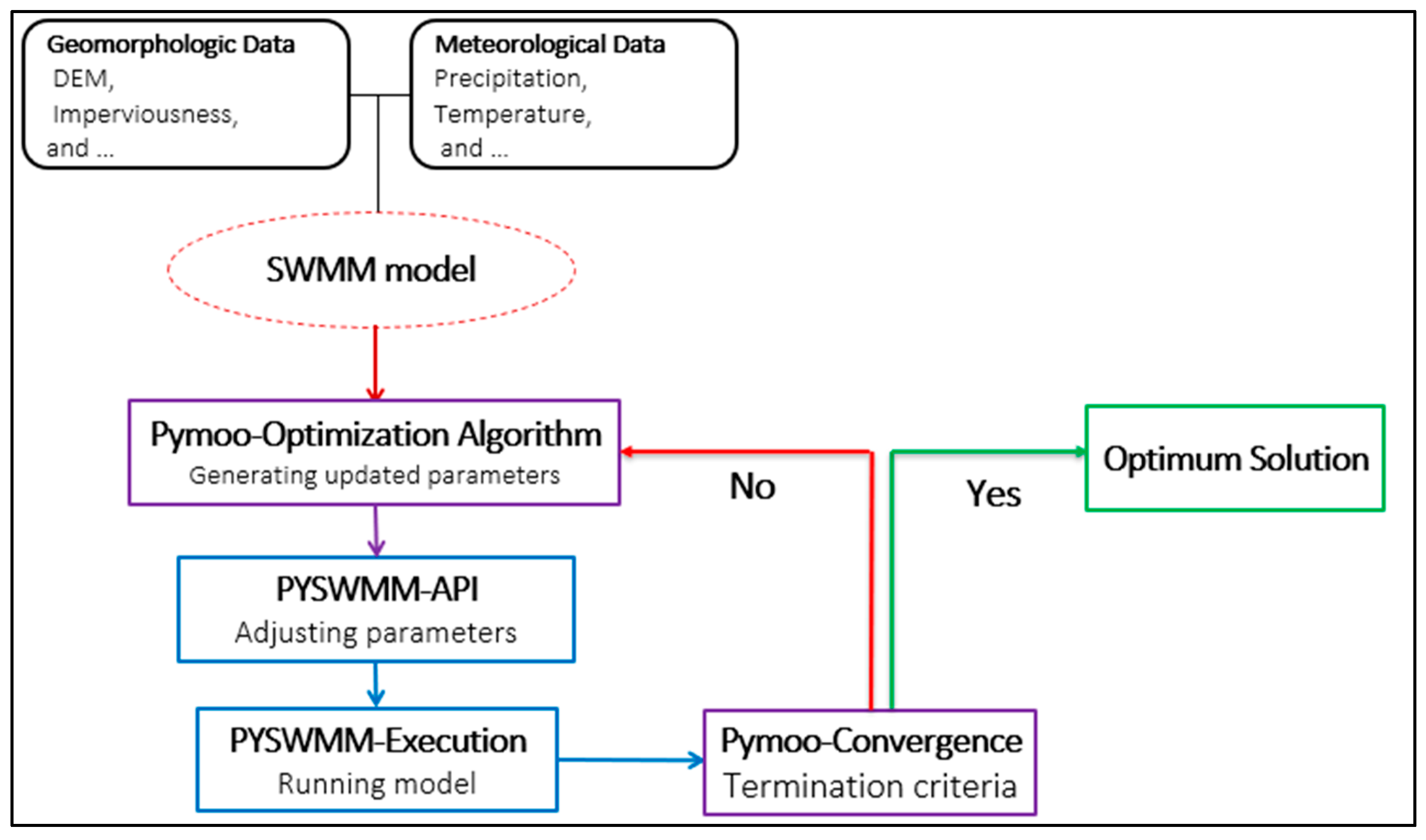
The integration between PySWMM and Pymoo, as illustrated in Figure 1, enables a seamless and dynamic exchange of data between the two modules. The calibration process using the integrated PySWMM–Pymoo framework follows the steps outlined below, which systematically link parameter generation, model execution, and performance evaluation in an automated loop.

Step 1: Model Setup and Parameter Identification

The SWMM model is developed using meteorological, geomorphological, and geographic data, followed by identification of influential parameters through sensitivity analysis for calibration.

Step 2: Generation of Candidate Parameters using Pymoo

The Pymoo optimization algorithm generates candidate parameter sets that represent potential combinations of influential parameters likely to improve model performance.

Step 3: Parameter Update via PySWMM API

Each parameter set is dynamically applied to the SWMM model using PySWMM’s API, enabling real-time updates without manual file editing and improving automation efficiency.

Step 4: Model Execution and Output Evaluation

The updated SWMM model is run using PySWMM, and simulated outputs are evaluated against observed data using objective functions.

Step 5: Performance-Based Optimization Search

The Pymoo optimization algorithm evaluates each solution using performance metrics and iteratively refines the search by favoring better-performing parameter sets.

Step 6: Convergence Check and Final Solution

The calibration iterates until termination criteria are met, returning an optimal parameter set that minimizes error between observed and simulated flows.

The presented automated calibration links model execution with optimization algorithms to improve simulation accuracy. It begins with defining objective functions, which are evaluated through repeated simulations as the optimizer explores parameter combinations. By iteratively adjusting parameters to minimize error, the process yields a well-calibrated model and offers a faster, more objective alternative to manual calibration, especially for complex, large-scale systems.

This study employs a single objective and multi-objective function for automatic calibration to assess the effectiveness of the PySWMM-Pymoo tool for calibrating SWMM. Of the several single-objective optimization algorithms available in the Pymoo package, (Particle Swarm Optimization) PSO and NSGAII were chosen for their ability to avoid local optima, adaptively adjust the search space, and globally optimize complex nonlinear functions, along with their robust convergence properties. This tool also leverages parallel computing to improve the convergence rate of the SWMM calibration process.

PSO is well-suited for single-objective problems involving nonlinear and continuous parameter spaces, offering efficient convergence and relatively low computational cost. NSGA-II was chosen for multi-objective calibration due to its ability to maintain solution diversity and generate a well-distributed Pareto front, making it ideal for balancing competing objectives such as NSE, PBIAS, and RSR. Both algorithms have been widely applied in environmental and hydrologic applications and are supported natively within the Pymoo framework, making them practical and effective choices for this study.

2.2. Case Study Description

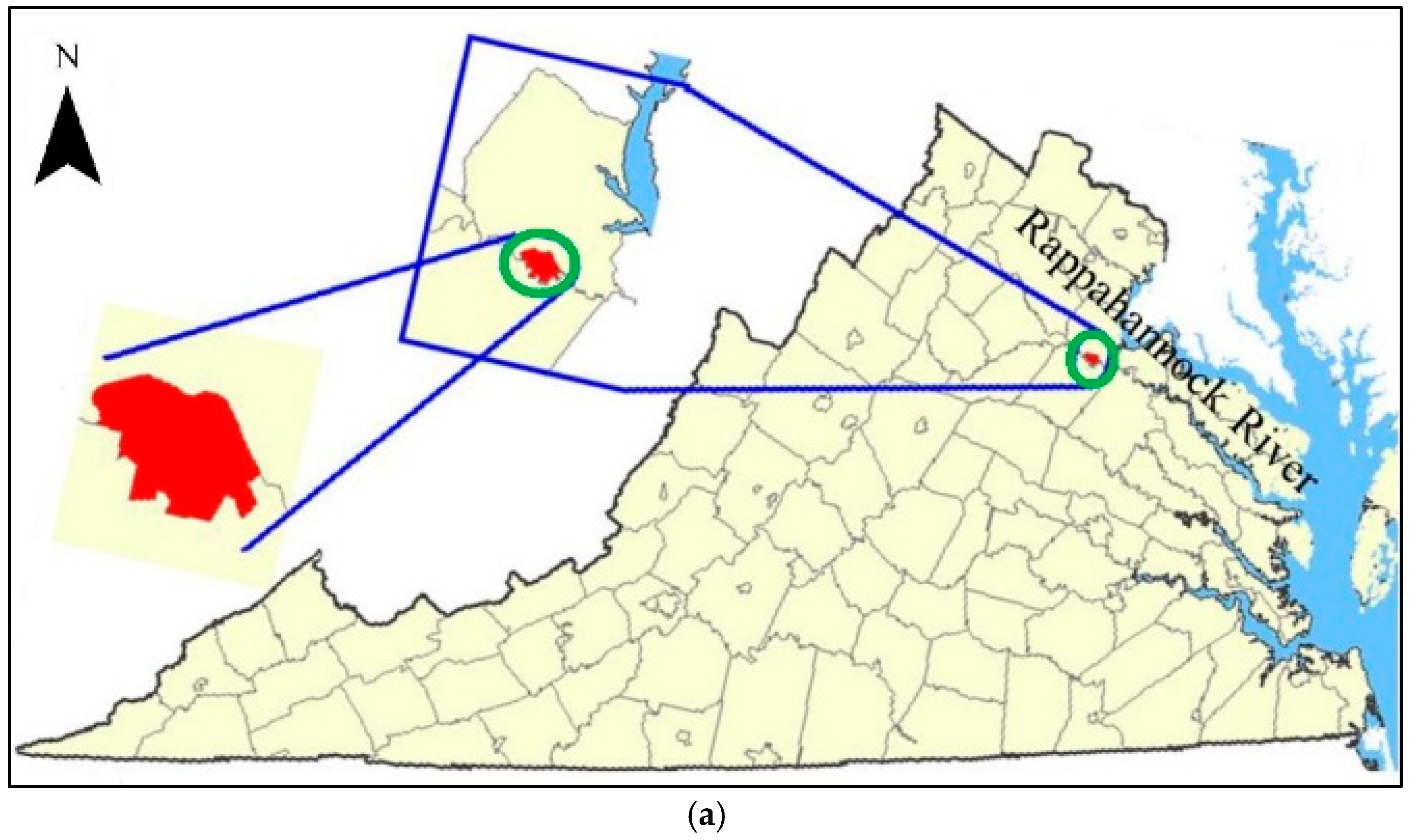
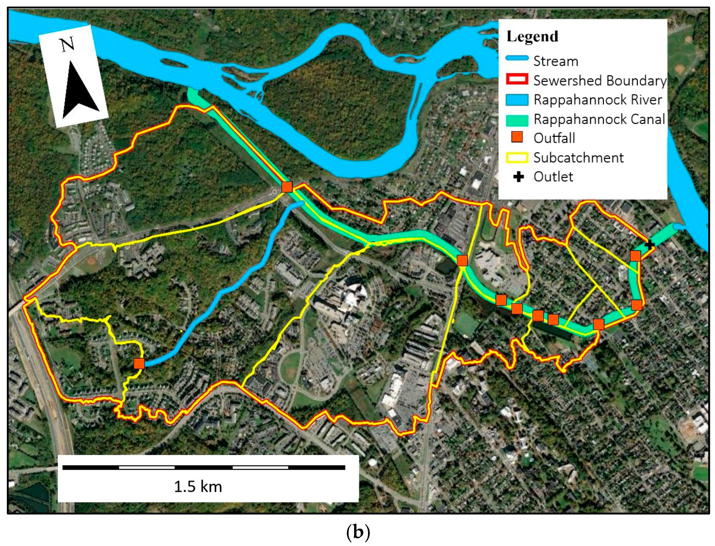
The study area lies within the City of Fredericksburg, VA (see Figure 2a) in northeastern Virginia that is tributary to the Rappahannock River and the Chesapeake Bay estuary. Fredericksburg is a relatively compact urban center located at the transition between Virginia’s Piedmont and Coastal Plain physiographic provinces. Within the City is the historic Virginia Electric Power Company (VEPCO) canal. Originally, the canal extended from a water intake on the Rappahannock River, upstream of the former site of Embry Dam, and discharged back into the river at a now defunct hydropower station. While the canal still follows its original course, the upstream dam has been removed, thus all inflows from the river have been blocked, so the only water entering the canal comes from either runoff from the contributing drainage area of the canal or it is pumped from the Rappahannock River. A pump station is present at the canal outlet to provide this capability. The contributing drainage area is known as the Canal sewershed. The location and boundary of the sewershed, along with the monitoring station, are shown in Figure 2b. Monitoring locations were established just upstream of the watershed outlet and at the point where the mainstream discharges into the canal. A sewershed is like a watershed, except it is in an urban area; often drainage boundaries are determined by roof lines and/or storm drains and conveyance.

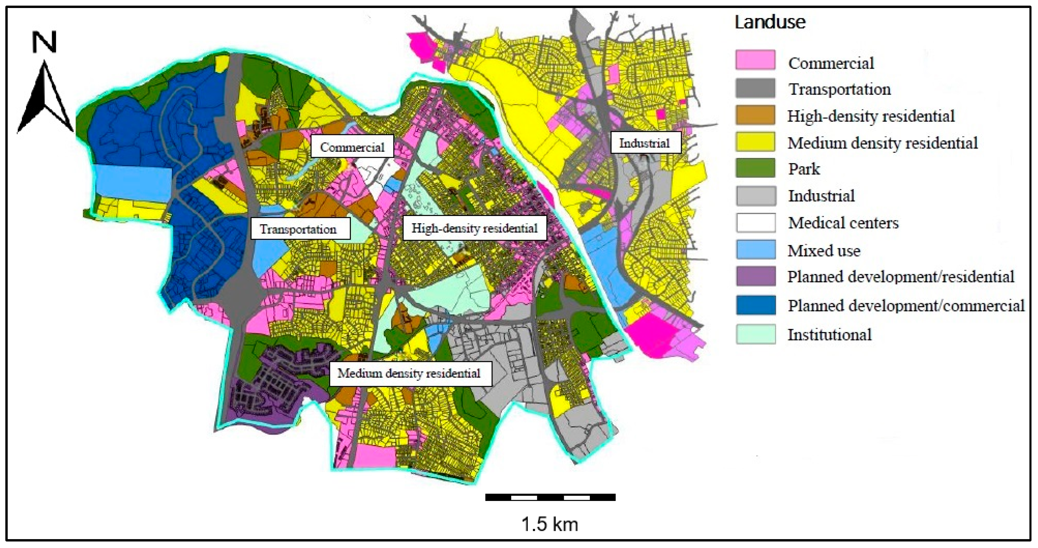
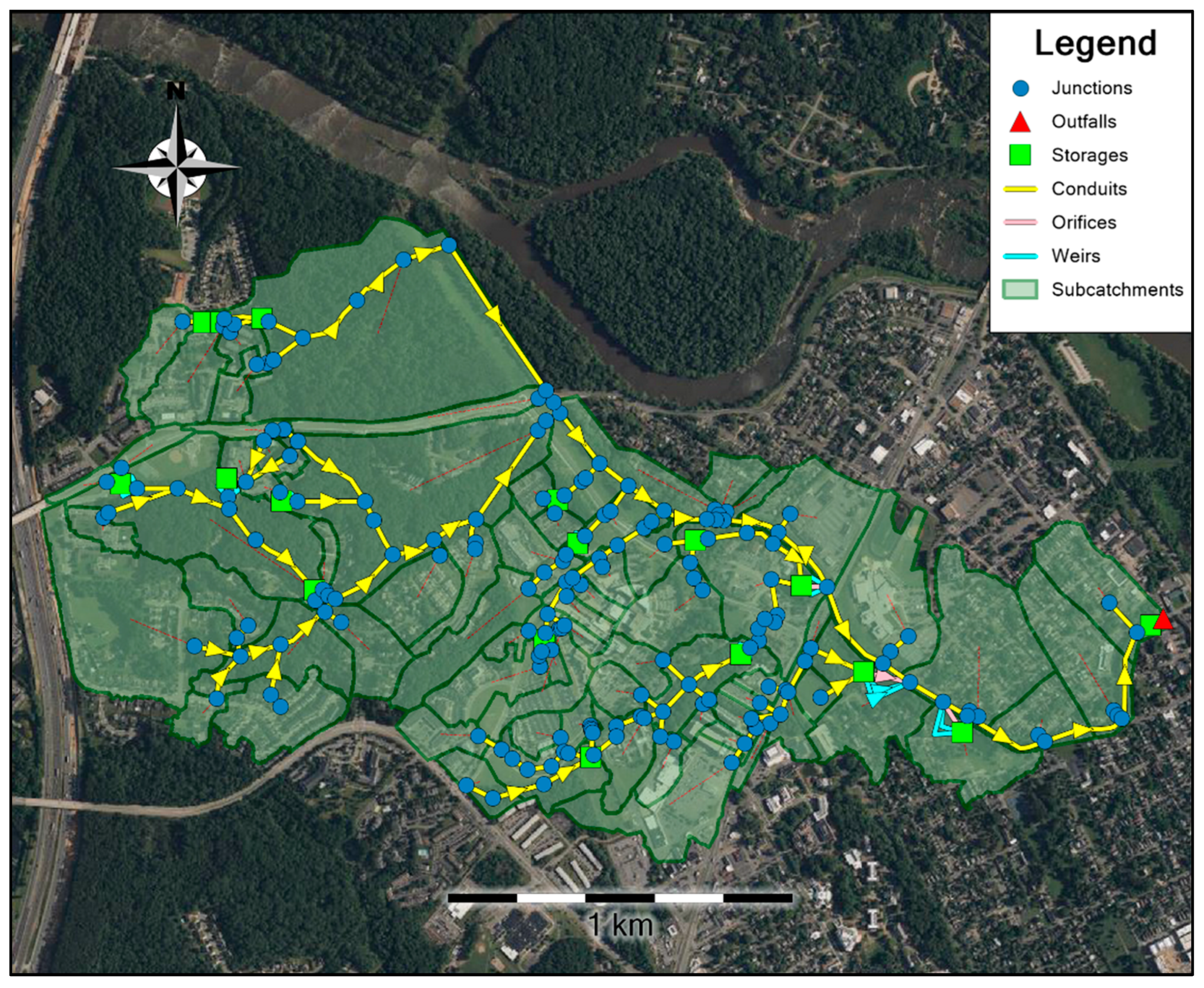
The canal sewershed spans 5.20 km² of highly urbanized area (Figure 3), featuring a mix of land uses including residential (30.2%), transportation (17.6%), commercial and medical center (12.2%), and industrial (7.1%). Breakdown of land use in the City of Fredericksburg is provided in

Table 1. Percentage of coverage for each land use class.

Landuse	Percentage of Coverage
Residential	30.2
Transportation	17.6
Commercial and medical centers	12.2
Planned development/commercial	11.0
Preservations and parks	10.2
Industrial	7.1
Institutional	4.7
Planned development/residential	3.7
Mixed-use	3.3

.

Long-term precipitation data from the nearby Corbin, VA station (USC00442009) indicate that the area experiences its wet season during late spring through summer. Monthly average precipitation from May to July is relatively high, ranging from 101 mm to 105 mm, and coincides with frequent convective storm activity. These months also record the highest number of days with rainfall ≥ 2.5 mm, occurring between 6.1 and 7.1 days per month, which reflects the frequency of storm events during this period. In contrast, the dry season begins around August, with average monthly precipitation decreasing and continuing to decline through November (85 mm) and December (92 mm), accompanied by fewer rainfall days and lower intensity. This seasonal variation allows the selected April–December period to capture a wide range of hydrological conditions, from high-intensity, short-duration events during the wet season to drier conditions with less frequent rainfall. Therefore, using this period for the study ensures that the model is calibrated for both storm runoff and base flow conditions under realistic seasonal variability.

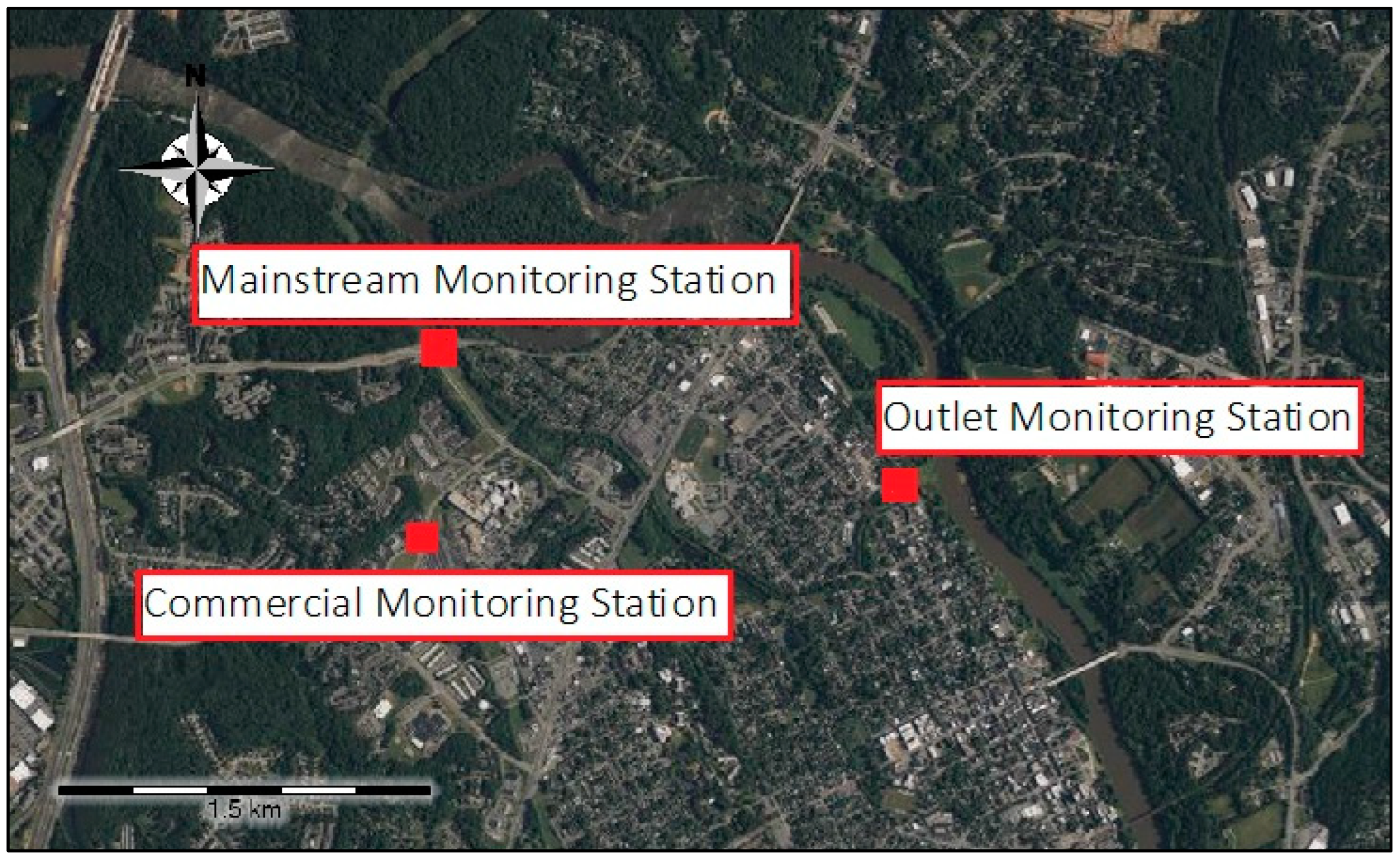
2.3. Monitoring

Several monitoring stations were installed within the sewershed and in nearby Fredericksburg to measure the quantity and quality of runoff during and immediately after storm events. For a complete description of these sites and results, the reader is referred to [7,57].

The monitoring locations used for model calibration are shown in Figure 4. These monitoring stations include just upstream of the watershed outlet, at the point where the main stream discharges into the canal, and within a subcatchment characterized by commercial land use.

2.4. Base SWMM Model

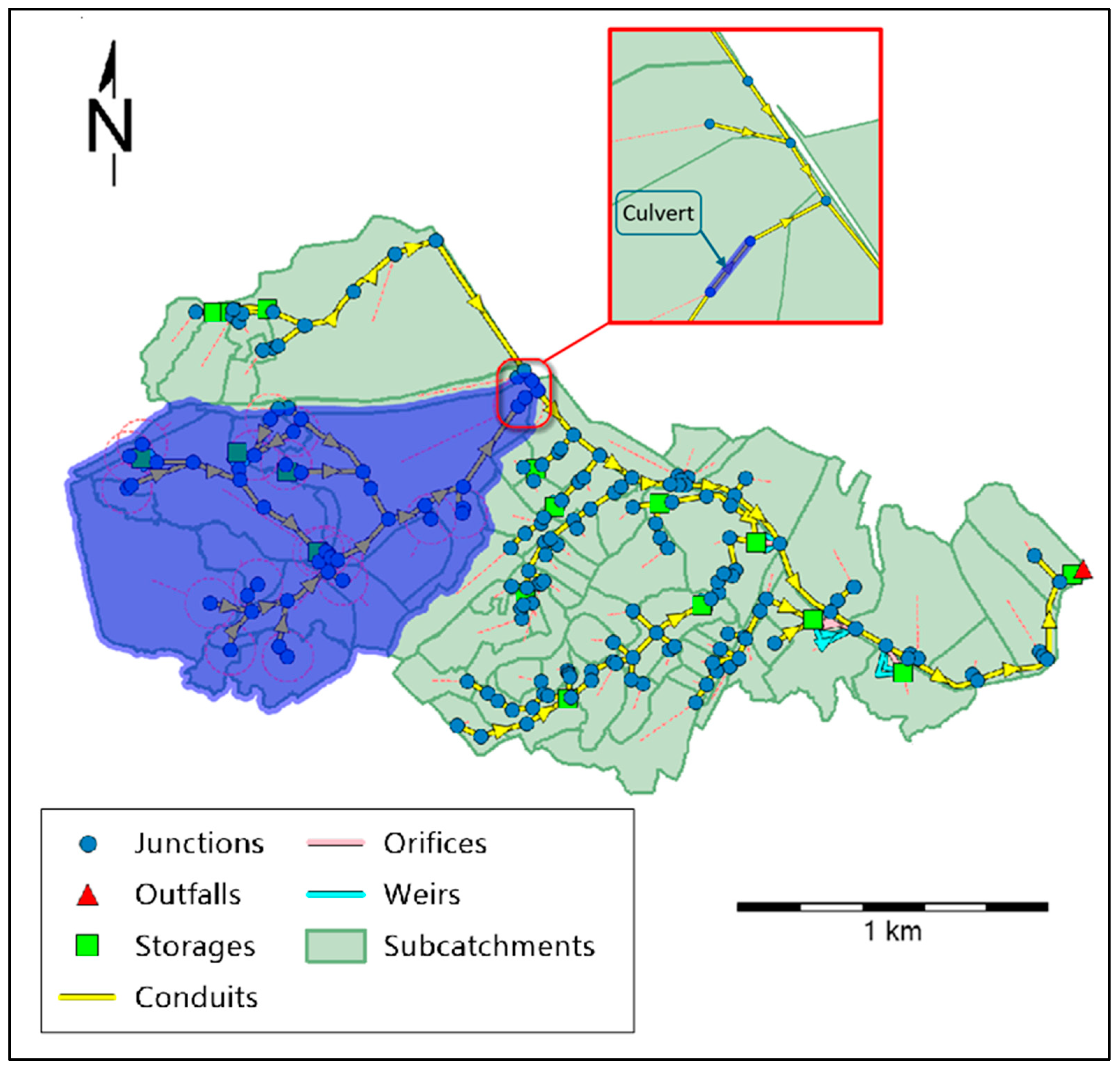
A SWMM model of the canal sewershed was developed based upon GIS data provided by the City of Fredericksburg, supplemented by field data of the conveyance network collected in summer of 2021. The model includes 74 sub-catchments, 156 conduits (links), and 156 nodes (junctions) [58]. ArcGIS Pro 2.8.2 was used to delineate the subcatchments based on a 1-m resolution Digital Elevation Model (DEM) supplied by the City of Fredericksburg [59].

The SWMM model also requires various inputs including precipitation, temperature, soil properties, hydraulic systems and infrastructure specifications, land use, and topography. Rainfall data were loaded into the model as a time series, demonstrating the rainfall volume recorded by rain gauges at the monitoring station. Temperature data were obtained from the closest NOAA station—Corbin, VA (station ID: USC00442009)—located approximately 15 km from Fredericksburg, VA, using recent records from the National Climatic Data Center (NCDC) [60]. The model simulates evaporation rates based on daily minimum and maximum air temperature.

The rainfall time series used for model input had a 5-min time step, which was selected to match the resolution of flow monitoring data and to accurately capture the short-duration, high-intensity rainfall events typical of urban stormwater systems.

The infiltration mechanism in SWMM was simulated using the Green-Ampt approach [61] and the parameters included in this method, such as suction head, hydraulic conductivity, and initial moisture deficit, were obtained from the Web Soil Survey Geographic (SSURGO) database provided by the U.S. Department of Agriculture Natural Resources Conservation Service [62].

The dynamic wave algorithm was chosen for flow routing in SWMM because it provides the most detailed and physically realistic simulation of flow hydraulics in urban drainage systems. Groundwater flow and interaction with surface water are simulated by a simplified Darcy’s law, which is driven by the aquifer bottom elevation, factors of groundwater-surface water interaction, unsaturated upper zone depth, saturated groundwater table elevation, aquifer porosity, and hydraulic conductivity in the saturated zone [63]. The elevation of the groundwater table was quantified using Digital Geologic Data for City of Fredericksburg and Spotsylvania County [64]. These parameters drive the flow between the aquifer and the stream, calculating the groundwater movement based on both the levels of the ground and surface water.

The model incorporated measured sub-hourly rainfall data and daily temperature data as input. The base model underwent partial manual calibration before starting automatic calibration.

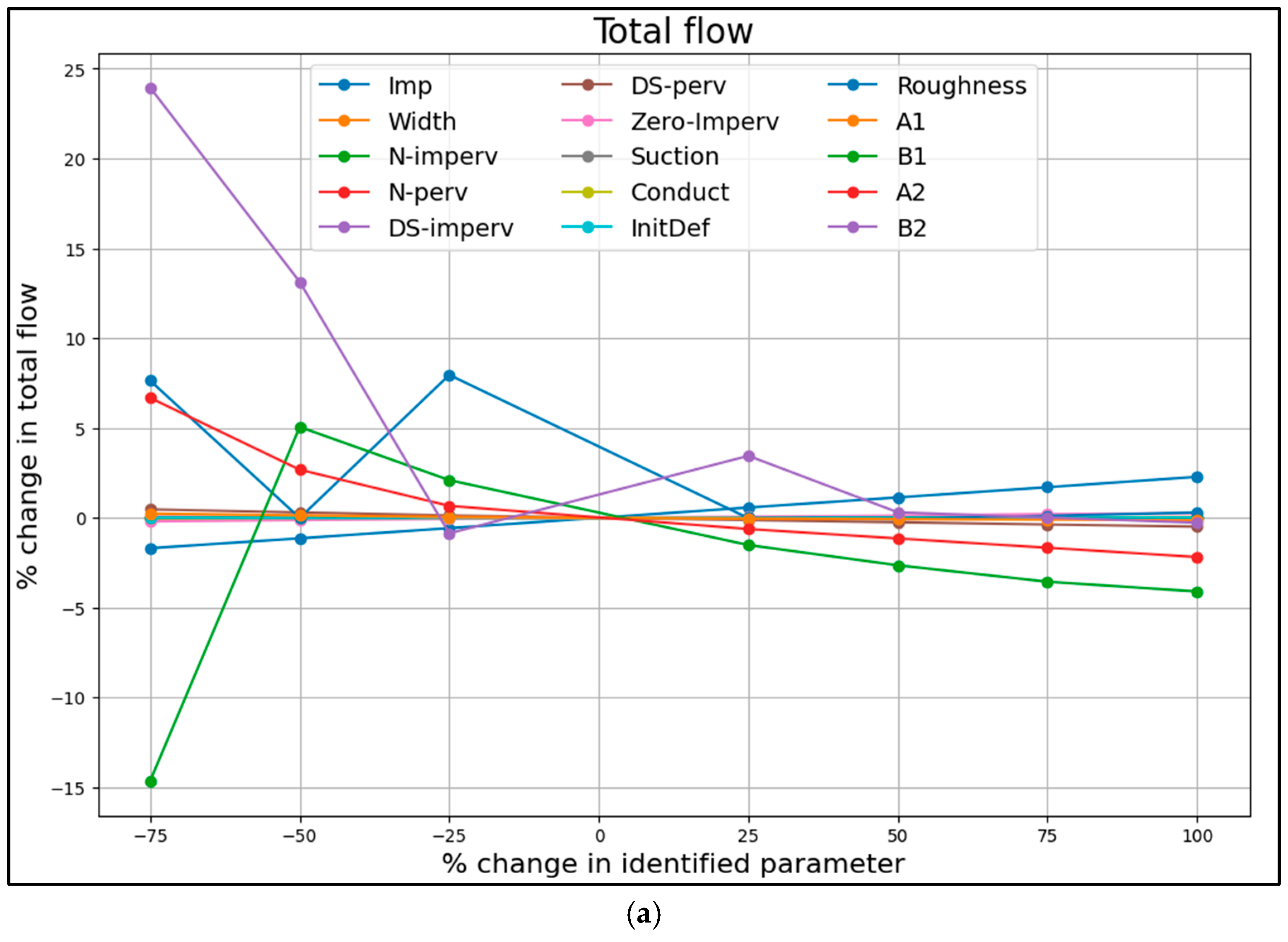
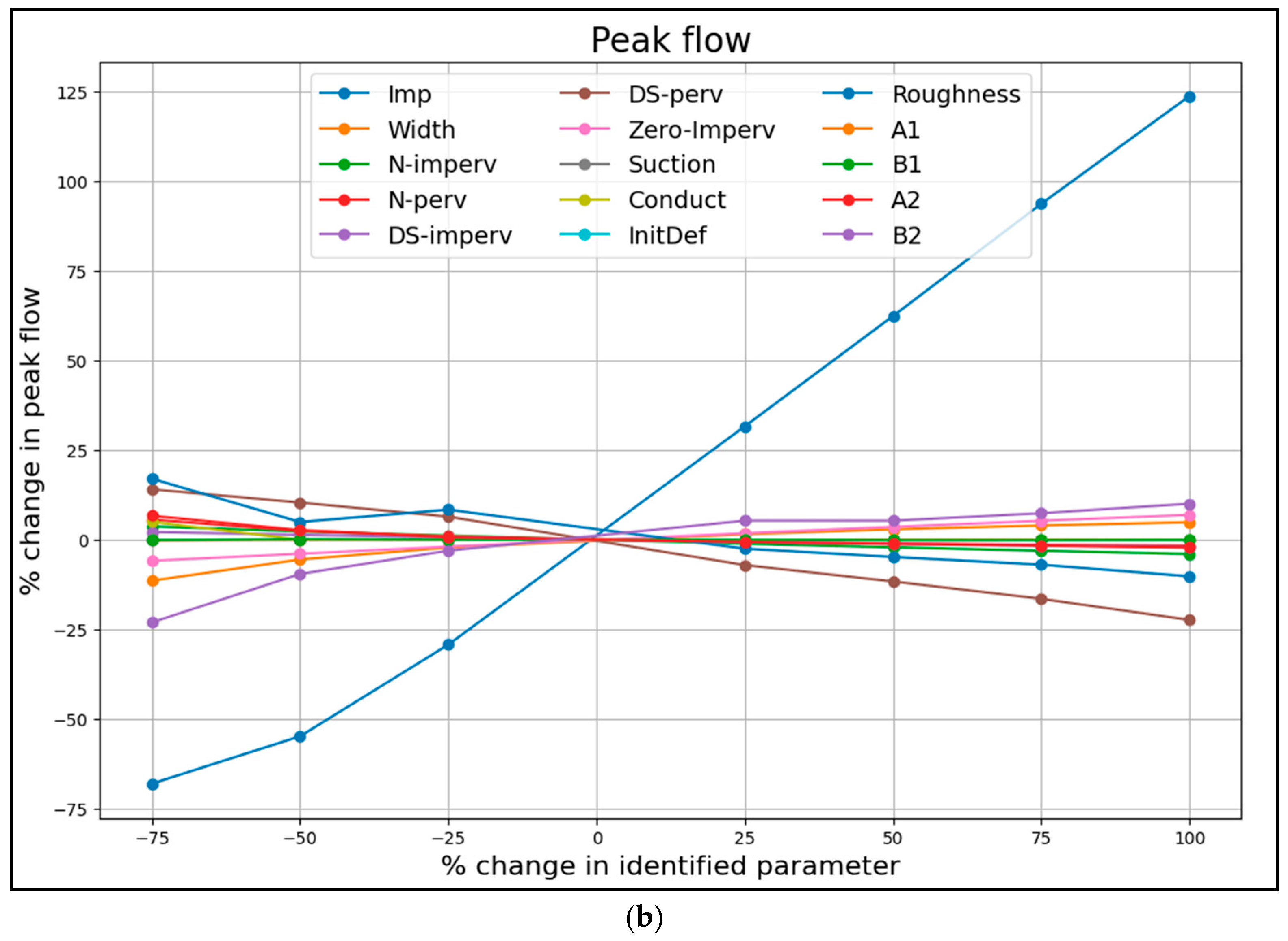
2.5. Sensitivity Analysis

In this study, the integrated PySWMM-Pymoo tool was employed to perform sensitivity analysis and automated calibration of the SWMM model for both single and multi-objective scenarios. Sensitivity analysis was conducted to identify the most impactful parameters, which were subsequently utilized in the calibration process by targeting these influential parameters.

Parameter sensitivity analysis was conducted using the one-at-a-time (OAT) approach, which involves varying each input parameter individually while keeping the others fixed. This method allows for the assessment of the impact of each parameter on the results, specifically examining the total flow over the entire simulation period and peak flow. By measuring and comparing these effects, we evaluated how each parameter influences overall flow behavior.

$$S_{total,i}\left(\%\right)={\displaystyle \frac{Qtotal\left(P_i+∆P_i,P_{j\ne i}=P_j^0\right)-Qtotal\left(P_i,P_{j\ne i}=P_j^0\right)}{Qtotal\left(P_i,P_{j\ne i}=P_j^0\right)}}\times 100$$

(1)

$$S_{peak,i}(\%)={\displaystyle \frac{Qpeak\left(P_i+∆P_i,P_{j\ne i}=P_j^0\right)-Qpeak(P_i,P_{j\ne i}=P_j^0)}{Qpeak(P_i,P_{j\ne i}=P_j^0)}}\times 100$$

(2)

where:

$S_{total,i}\left(\%\right)$ = Sensitivity of the total flow to the input P_i parameter

$S_{peak,i}(\%)$ = Sensitivity of the peak flow to the input P_i parameter

Qmean = Overall average of the flow rate over the simulation period

Qpeak = Maximum flow rate over the simulation period

P_i = Input Parameter

∆P_i = Increment applied to P_i

P_j⁰ = Baseline (original) values of all other input parameters P_j where j ≠ i

The range of each parameter used in the sensitivity analysis was determined based on a combination of sources, including recommendations from the SWMM user manual, parameter values commonly reported in peer-reviewed studies, and practical modeling experience from previous applications in urban watersheds with similar land use and hydrologic characteristics.

While the OAT sensitivity analysis method has known limitations, particularly its inability to account for interactions between parameters, we selected it for this study due to its computational efficiency, simplicity, and ease of interpretation, which make it well-suited for the initial development and demonstration of the calibration tool.

2.6. Hydrologic Calibration and Validation

The model was calibrated using flow data collected from 15 April to 30 December 2021—a period that encompasses both the wet and dry seasons in the study area. This timeframe includes months characterized by frequent, high-intensity storm events as well as periods with lower-intensity but more sustained rainfall. As a result, the calibration captures a wide spectrum of hydrologic conditions, enabling the model to simulate both peak storm flows and base flow conditions with greater accuracy and reliability. Calibration is a critical step in enhancing the accuracy and reliability of hydrological simulations, as it involves adjusting model parameters to closely match observed data. To guide this process, a sensitivity analysis was first performed to identify the parameters that have the greatest influence on model performance. Once these key parameters were identified, optimization techniques were used to refine them. Depending on the calibration goals, either single-objective or multi-objective optimization methods can be applied. Single-objective optimization focuses on improving one performance metric, while multi-objective optimization considers multiple metrics simultaneously to achieve a more balanced and comprehensive calibration. In this study, the NSGA-II algorithm was applied for multi-objective optimization, while the PSO algorithm was used for single-objective optimization tasks.

The objective formulation considered in this study was minimizing total flow volume error. NSE, PBIAS, and RSR have been employed as metrics that assess aspects of the performance of the calibrated model. The near-optimal results represent a balance among these metrics [65].

$$NSE=1-{\displaystyle \frac{\sum _{i=1}^n{\left(O_i-P_i\right)}^2}{\sum _{i-=1}^n{\left(O_i-\overline{O}\right)}^2}}$$

(3)

$$PBIAS={\displaystyle \frac{\sum _{i=1}^n\left({P_i-O}_i\right)}{\sum _{i=1}^n{O}_i}}\times 100$$

(4)

$$RSR={\displaystyle \frac{RMSE}{STDE{V}_{obs}}}={\displaystyle \frac{\sqrt{\sum _{i=1}^n{\left(O_i-P_i\right)}^2}}{\sqrt{\sum _{i=1}^n{\left(O_i-\overline{O}\right)}^2}}}$$

(5)

where:

O_i = Observed flow at time

P_i = Predicted flow at time

$\overline{O}$ = Mean of the observed flow

n = Number of observations

After completing calibration, the model was run for a validation period to assess its performance and ensure its accuracy. Validating a SWMM model after calibration is essential to ensure it performs reliably. This involves testing the model using independent datasets that were not part of the calibration process. By applying the same metrics including NSE, PBIAS and RSR, the validation process checks whether the model can accurately reproduce observed data under different conditions.

2.7. Stepwise Calibration Approach

In this study, a systematic and robust stepwise calibration approach was employed to calibrate the SWMM model for a large and complex urban sewershed. The sewershed consists of multiple drainage paths and subcatchments, which collectively form smaller sub-sewersheds, each contributing uniquely to the overall hydrologic response. To manage model complexity and improve efficiency, calibration began by selecting a representative subset of subcatchments, those directly contributing to the mainstream flow and supported by available monitoring data. This subset was used to calibrate key hydrologic parameters, particularly those governing infiltration and base flow, under observed conditions.

Once satisfactory calibration was achieved for this subset, the calibrated parameters, especially those related to base flow and infiltration, were transferred to similar subcatchments throughout the rest of the sewershed. This transfer was justified based on comparable land use, soil characteristics, and drainage patterns across subcatchments. Although spatial variability exists, this assumption is common in urban hydrologic modeling where monitoring data are limited. It allows for hydrologic consistency across the watershed while reducing computational burden and calibration time. The final model was then refined by calibrating influential parameters at the full sewershed scale to ensure accurate representation of both localized responses and cumulative watershed behavior. This stepwise method not only streamlines the calibration process but also enhances model reliability and efficiency.

In the optimization approach, the calibration process is enhanced by transitioning from a floating-point format to an integer-based representation for certain parameters. This technique effectively reduces the search domain by discretizing real-valued parameters to integers or restricting them to a specific number of decimal places. By doing so, the optimization process becomes more efficient, as it focuses on a narrower, predefined parameter space. This method not only simplifies the computational process but also ensures that the calibration aligns more closely with realistic, practical values, improving the overall accuracy and reliability of the model.

3. Results and Discussion

3.1. Sensitivity Analysis Results

Sensitivity analysis was conducted to narrow the set of parameters included in the calibration process [66,67]. This analysis aimed to evaluate the relative influence of individual SWMM input parameters on simulated flow, to distinguish influential and non-influential parameters. In SWMM-based studies, sensitivity analysis is a common practice, often implemented using the OAT method, where each input parameter varies while others remain constant—being the most prevalent technique [47,68].

A literature review revealed that the most sensitive parameters are often site-specific. Based on the prior literature [7,11,20,24,69,70], the guidelines from the SWMM model manual, and practical modeling experience, 15 hydrological parameters have been consistently recognized as influential and are frequently cited in various studies. The parameters and their specific ranges are detailed in

Table 2. Selected input parameters for sensitivity analysis.

Category	Parameter	Physical Effect	Range	Unit
Subcatchments Characteristics	Imp	The percentage of land in a sub-catchment that is characterized by impervious cover.	[0.0, 100]	%
	Width	The width of the surface flow path contributes to sheet flow within a subcatchment.	[100, 10,000]	m
	N-imperv	Manning’s n for overland flow over the impervious portion of a given subcatchment.	[0.01, 0.05]	_
	N-perv	Manning’s n for overland flow over the pervious portion of a given subcatchment.	[0.01, 0.5]	_
	DS-imperv	Depth of depression storage on the impervious portion of a given subcatchment.	[0.5, 3]	mm
	DS-perv	Depth of depression storage on the pervious portion of a given subcatchment.	[1, 6]	mm
	Zero-Imperv	Percent of the impervious area of a given sub-catchment without any capacity for depression storage.	[18, 32]	%
Infiltration Characteristics	Suction	Percent of the impervious area of a given sub-catchment without any capacity for depression storage.	[12, 110]	mm
	Conduct	Saturated hydraulic conductivity of soil used in the Green-Ampt method.	[20, 200]	mm/h
	InitDef	Initial moisture shortfall in the soil for the Green-Ampt infiltration model.	[0.1, 0.56]	_
Conduit Characteristics	Roughness	Manning’s roughness coefficient assigned to a specific conduit or open channel.	[0.011, 0.015]	_
Groundwater Characteristics	A1	Groundwater flow coefficient.	[0, 1]	_
	B1	Groundwater flow exponent.	[0, 10]	_
	A2	Groundwater flow coefficient.	[0, 1]	_
	B2	Groundwater flow exponent.	[0, 10]	_

.

The chosen parameters characterize subcatchments, channels, and the flow of groundwater and surface water. Imp, width, N-imperv, N-perv, DS-imperv, DS-perv and Zero-Imperv are associated with subcatchment properties. Suction, Conduct, and InitDef are Green-Ampt equation parameters that represent soil infiltration characteristics. Roughness or conduit’s Manning’s n represents the resistance to water flow within a conduit. A1, B1, A2, and B2 are groundwater and surface water flow parameters that determine the rate of lateral groundwater flow between the aquifer and the node. These coefficients calculate groundwater flow based on the levels of groundwater and surface water.

By making tweaks to each parameter, the resulting changes in simulated peak flow and total flow volume at the sewershed outfall were compared to the values from the manually calibrated model. The percentage changes, representing the parameter sensitivities, were then sorted, ranked (as shown in

Table 3. Rank of input parameters for sensitivity analysis.

Parameter	Total Flow Volume		Peak Flow
	Maximum Percentage Variation	Rank	Maximum Percentage Variation	Rank
Imp	2.29	5	123.67	1
Width	−0.04	10	−11.42	5
N-imperv	0.03	11	−3.97	10
N-perv	0.03	12	5.63	8
DS-imperv	−0.49	6	−22.35	3
DS-perv	0.048	9	2.17	11
Zero-Imperv	0.25	7	6.93	6
Suction	0.00001	15	0.00001	15
Conduct	0.004	13	4.99	9
InitDef	−0.0001	14	−0.0001	14
Roughness	7.96	3	17.01	4
A1	0.23	8	−0.12	13
B1	−14.64	2	0.13	12
A2	4.93	4	6.67	7
B2	23.95	1	−23.04	2

), and the results of the sensitivity analysis of parameters are provided in Figure 5.

The maximum percentage variation represents the highest relative change in total flow volume or peak flow resulting from individual parameter adjustments, and was calculated using Equations (1) and (2) under different incremental changes applied to each parameter.

Input parameters were identified as influential based on the magnitude of their impact on model outputs. Consistent with the method used by Barco et al. (2008) [70], the ranking was determined using the maximum percentage change as the evaluation metric (Table 3).

The parameters with the greatest impact on model outputs for total flow volume and peak flow were identified as the most influential, with their sensitivity varying between these metrics, as shown in Figure 5. Sensitivity analysis results show the parameter associated with imperviousness, and groundwater has the most impact on both total flow volume and peak flow. In this study, by evaluating the impact of each parameter on both total flow volume and peak flow, the 13 parameters including Imp, Width, N-imperv, N-perv, DS-imperv, DS-perv, Zero-Imperv, Conduct, Roughness, A1, B1, A2, and B2 were identified as influential parameters and were subsequently used for the calibration of the SWMM model.

3.2. SWMM Model Calibration Results

The model was calibrated using a selection of influential parameters with appropriate search bounds for each. The objective was to minimize errors between predicted and observed values.

In this study, an evolutionary algorithm was employed for model calibration. This optimization method iteratively explores each parameter’s domain by generating a population of potential solutions, evaluating their performance, and selecting the fittest individuals to form the next generation. Through successive generations, the algorithm refines the search, gradually converging on the optimal or near-optimal solution within the parameter domain.

Two examples, one of single-objective optimization and one of multi-objective optimization, are presented in the following section to demonstrate the model’s ability to calibrate using either a single objective function or multiple objective function.

3.2.1. Single Objective Calibration

In this section, the SWMM model for the entire sewershed, including 74 sub-catchments (Figure 6), was calibrated using a single objective function.

Calibrating a SWMM model for a sewershed is performed through an effective and systematic approach by starting with a smaller portion of the sewershed containing several subsets of subcatchments. The first step involves selecting subcatchments that directly contribute to the mainstream in the sewershed and focusing on calibrating this portion of the entire sewershed. This simplifies the system and allows for more precise calibration of both base flow during dry periods and storm peak flow during wet periods.

The rationale for selecting this subset of subcatchments lies in their hydrologic significance and data availability. This portion of the sewershed contains a monitoring station at its outlet, enabling reliable calibration against observed flow data. Because these subcatchments are the main contributors to streamflow in the canal, the calibrated base flow and infiltration parameters derived from this area provide a strong foundation. These parameters were then extended to the remaining subcatchments based on hydrologic similarity. Given the comparable land use, soil types, and drainage infrastructure across the sewershed, this approach allowed for effective parameter transfer while maintaining physical relevance. Subsequent full-system optimization ensured that the transferred parameters were further refined and adapted to local conditions, supporting both model accuracy and computational efficiency.

A subset of 19 subcatchments within this sewershed was selected for calibration of base flow parameters. These subcatchments contribute to the mainstream of the sewershed, which ultimately discharges into the canal, as illustrated in Figure 7.

This section of the sewershed, comprising 19 selected subcatchments, drains into the canal through a culvert and conduit at the confluence point. Streamflow measurements were taken at the culvert inlet. By using observed flow values at the downstream of this portion of the sewershed, the model can be calibrated to simulate both base flow and storm flow. Once this subset of subcatchments is calibrated, the calibrated base flow parameters were applied to the rest of the sewershed.

The transferability of calibrated parameters across the sewershed is supported by the similarity in physical and hydrologic characteristics among the subcatchments, including land cover, impervious surface coverage, and drainage configurations. The base flow and infiltration parameters, initially calibrated using observed data from a representative subset of subcatchments, were applied to the remaining areas with comparable conditions.

The objective function focused on maximizing NSE and utilized the PSO optimization algorithm to determine the calibrated parameters. The PSO works by simulating a group of particles (potential solutions) that move through the parameter space, guided by both their own best-known positions and the best-known positions of the swarm as a whole. Over multiple iterations, the particles adjust their positions, converging on the near-optimal solution based on collective and individual experience.

The optimization algorithm was configured to use 25 swarms with 200 iterations to calibrate the SWMM model of the entire sewershed. The initial calibration began with a manually calibrated model that had an NSE value of 0.22. As the iterations progressed, the NSE value improved, demonstrating the effectiveness of the optimization process.

The algorithm employed two termination criteria: the first was a maximum number of iterations, set at 200, and the second was based on convergence tolerance. Specifically, the algorithm would terminate if the improvement in the objective value fell below a threshold of 0.0001 for 30 consecutive iterations. The convergence behavior of the PSO algorithm over generations is illustrated in Figure 8. The convergence behavior shown in Figure 8 illustrates how the PSO algorithm progressively improves the objective function (NSE) over successive iterations. The steady upward trend in the curve reflects the automatic calibration tool’s ability to explore the parameter space and converge toward an optimal or near-optimal solution. The flattening of the curve near the final iterations indicates that the algorithm is reaching stability, with minimal improvement in NSE, which satisfies the convergence threshold. This demonstrates the effectiveness of the PSO in calibrating the model with reasonable computational efficiency.

To calibrate the model, observations from the outlet of the sewershed were utilized. The results of the calibration over two calibration and validation periods are shown in Figure 9.

The calibration process was demonstrated to be highly effective, with prediction results closely aligned with the observed data for both the calibration and validation periods, as illustrated in Figure 9. This indicates that the model accurately captures the underlying system dynamics, leading to reliable predictions.

The predicted and observed peak flows and total flow volumes at 5-min intervals, obtained through single-objective optimization, are presented in

Table 4. Predicted and observed maximum peak flows at 5-min intervals during the calibration and validation periods from single objective calibration.

Date	Category	Peak Flow (cms)		Time To Peak (min)
		Prediction	Observation	Prediction	Observation
26 July 2021	High Flow	0.339	0.308	65	70
17 August 2021	High Flow	0.246	0.238	135	120

and

Table 5. Predicted and observed flow volume at 5-min intervals during the calibration and validation periods from single objective calibration.

Date	Category	Flow Volume (m3)
		Prediction	Observation
19 July 2021–20 July 2021	Low Flow	1.68	1.71
17 August 2021–18 August 2021	Low Flow	4.2	4.35

. These results highlight the model’s ability to accurately replicate both storm event peaks, time to peak, and base flow conditions. The tables include data for both the calibration and validation periods, allowing for a clear comparison of the model performance in capturing maximum streamflow as well as low-flow behavior. The strong agreement between observed and predicted values demonstrates the model’s effectiveness in simulating short-duration, high-intensity storm events, crucial for flood risk assessment and stormwater planning. Additionally, the accurate representation of low-flow conditions supports long-term model reliability and is essential for evaluating water quality and baseflow-related processes.

3.2.2. Multi-Objective Calibration

To demonstrate the capability of the integrated link in calibrating the SWMM model based on multi-objective functions, a commercial subcatchment within the study area was selected. This is a small subcatchment within the larger sewershed, characterized by commercial land use, covering an area of 2630.5 m². This subcatchment includes 5 conduits and 6 junctions, as displayed in Figure 10. A monitoring station was located at the outlet of this subcatchment, recording water flow at 5-min intervals. This data is used as observations to compare with predicted flow and was used to calibrate the SWMM model.

To calibrate the SWMM model for the commercial subcatchment, three objective functions (f1, f2, and f3) were defined: maximizing NSE (f1), minimizing PBIAS (f2), and minimizing RSR (f3). The NSGA-II algorithm was used to optimize these objectives and identify the best solution. The algorithm generates some population based on different combinations of input parameters and then ranks these solutions into fronts based on dominance, with the first front comprising the non-dominated solutions. NSGA-II was then applied with crossover and mutation to evolve the population while maintaining diversity through a crowding distance mechanism. Over successive generations, the algorithm converges with a set of optimal trade-off solutions, known as the Pareto front.

The Pareto front in this multi-objective calibration example represents a set of near-optimal solutions for the three functions, highlighting the trade-offs between the competing objectives. The Pareto front with different objectives of this example is shown in Figure 11. The Pareto front resulting from the NSGA-II multi-objective optimization illustrates the trade-offs among NSE, PBIAS, and RSR. Each point on the Pareto front represents a non-dominated solution where improvement in one objective would lead to a compromise in another. The spread of solutions along the Pareto front reflects the optimization algorithm’s ability to maintain diversity in the population while approaching optimal trade-offs. This flexibility is essential in urban hydrologic modeling, where stakeholders may prioritize different aspects of model performance depending on the performance metric. The results of muti-objective calibration (Figure 11) show that increasing NSE values are generally associated with decreasing RSR, indicating improved model accuracy and a better match between observed and simulated flows. However, as NSE increases, PBIAS also tends to increase, suggesting a rising bias, reflecting underestimation in the model output. This trade-off reveals that while the model improves its overall efficiency (higher NSE) and reduces the residual error ratio (lower RSR), it may do so at the expense of increased bias. These trends highlight the need to balance multiple objectives in calibration, as optimizing one metric can sometimes lead to compromises in others.

To evaluate the accuracy and reliability of the calibrated model, its results were compared to observed data from both the calibration and validation periods, as shown in Figure 12. The comparison of calibrated and measured flow processes across four rainfall events indicates that the NSE, PBIAS, and RSR values are within acceptable ranges. This demonstrates a strong agreement between the simulated and observed flows.

The results for calibration and validation periods for the multi-objective calibration are provided in

Table 6. Statistical indices of streamflow during calibration and validation periods, based on results from the multi-objective optimization.

Statistical Index	Calibration	Validation	Model Performance
NSE	0.73	0.86	Good/Very good
PBIAS (%)	17.1	13.1	Good
RSR	0.52	0.37	Good/Very good

.

The comparison of simulation results, presented in Figure 12 and Table 6, indicates that the automatic calibration tool effectively calibrates the SWMM model to predict runoff for both the calibration and validation periods. The results, based on the criteria by Moriasi et al., 2007 [65], fall into the “Good” and “Very good” categories for calibration and validation periods, respectively.

The predicted and observed peak flows, time to peak, and total flow volumes at 5-min intervals during the calibration and validation periods, obtained through multi-objective optimization, demonstrate the model’s ability to effectively capture both high-flow and low-flow conditions (

Table 7. Predicted and observed maximum peak flows at 5-min intervals during the calibration and validation periods from multi-objective calibration.

Date	Category	Peak Flow (×103 cms)		Time To Peak (min)
		Prediction	Observation	Prediction	Observation
4 June 2021	High Flow	32.73	35.68	35	30
22 June 2021	High Flow	7.84	7.36	15	10

and

Table 8. Predicted and observed flow volume at 5-min intervals during the calibration and validation periods from multi-objective calibration.

Date	Category	Flow Volume (×103 m3)
		Prediction	Observation
3 June 2021–5 June 2021	Low Flow	55.24	56.91
17 June 2021–18 June 2021	Low Flow	110.85	118.92

). The close agreement between observed and simulated values highlights strong model performance, which is critical for accurate flood risk assessment and stormwater infrastructure planning. In addition to replicating peak flow behavior, the model also captures low-flow dynamics, which are important for base flow estimation and water quality modeling. These results further support the reliability and robustness of the model calibrated through the multi-objective optimization framework.

4. Conclusions

This study introduces a novel calibration tool for SWMM by integrating PySWMM with Pymoo. This tool capitalizes on the capabilities of PySWMM, Pymoo, and Python for automated calibration. This developed tool is designed to leverage PySWMM’s API capabilities for systematic adjustments of SWMM model parameters, while utilizing Pymoo’s advanced optimization algorithms to be able to use parallel search techniques to efficiently identify near-optimal values. The PySWMM-Pymoo tool supports both single and multi-objective automated calibration, making it suitable for event-based and continuous simulations. Furthermore, the tool performs sensitivity analysis prior to calibration, identifying influential parameters specific to the study area.

The PySWMM-Pymoo tool was applied in a case study sewershed in Fredericksburg, VA, demonstrating its feasibility and applicability. The developed tool was applied to calibrate a single subcatchments using multi-objective calibration and an entire catchment’s sewershed using single-objective calibration.

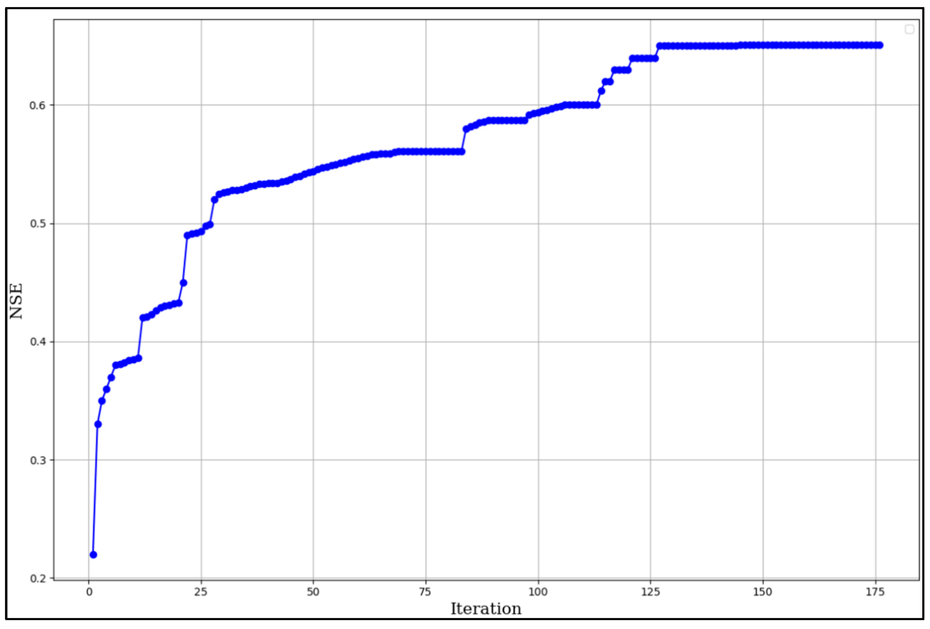
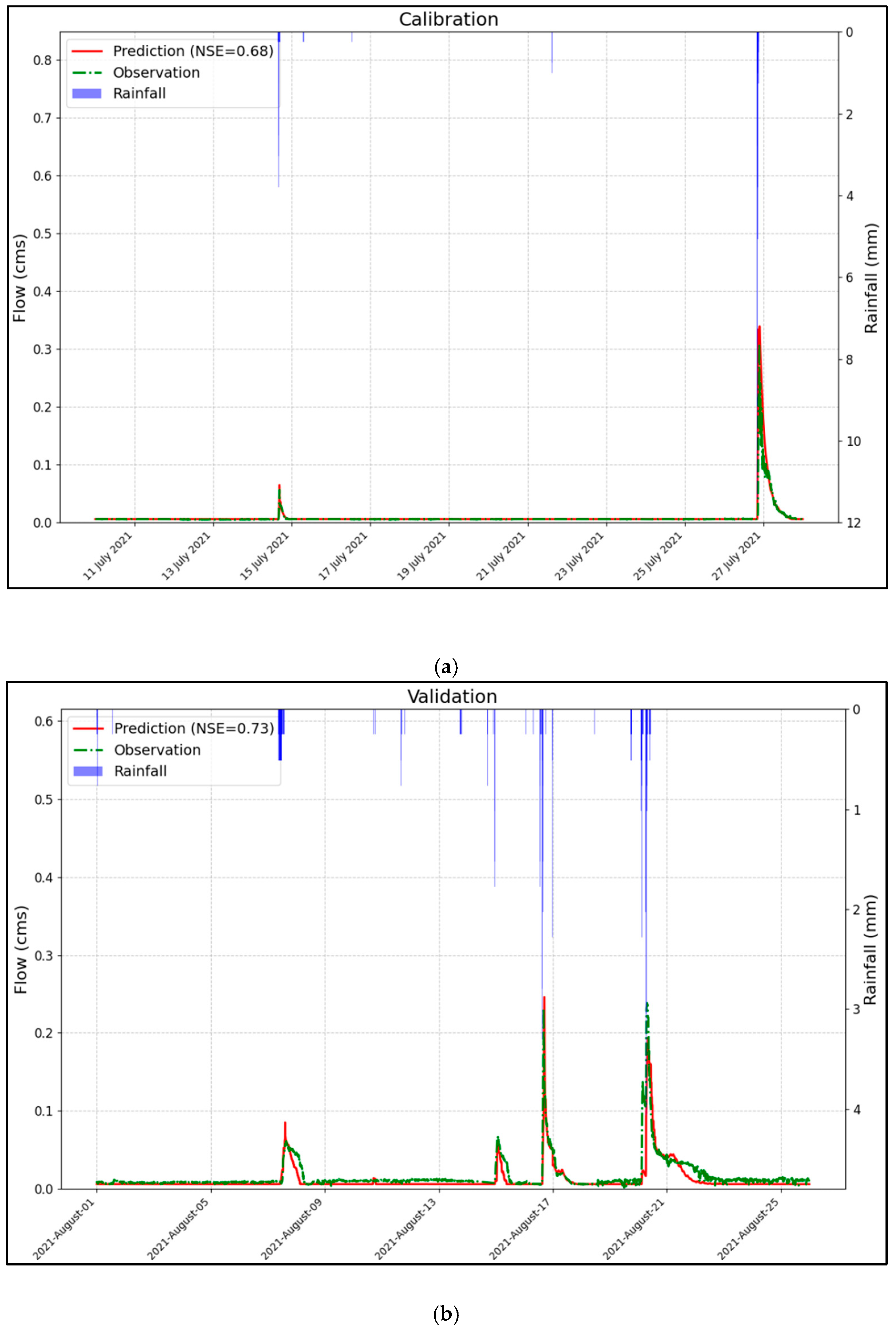
In single-objective optimization, the PSO algorithm was employed to maximize the NSE value. Calibrating the SWMM model for the entire sewershed followed a systematic and efficient approach, starting with a smaller section of the sewershed comprising a group of subcatchments that are the primary contributors to runoff. The parameters were fine-tuned for this group of subcatchments and then extended to the entire sewershed for comprehensive calibration. The NSE values from this test case for the calibration and validation phases were 0.68 and 0.73, respectively, demonstrating the reliability of the tool in achieving accurate calibration of the SWMM model.

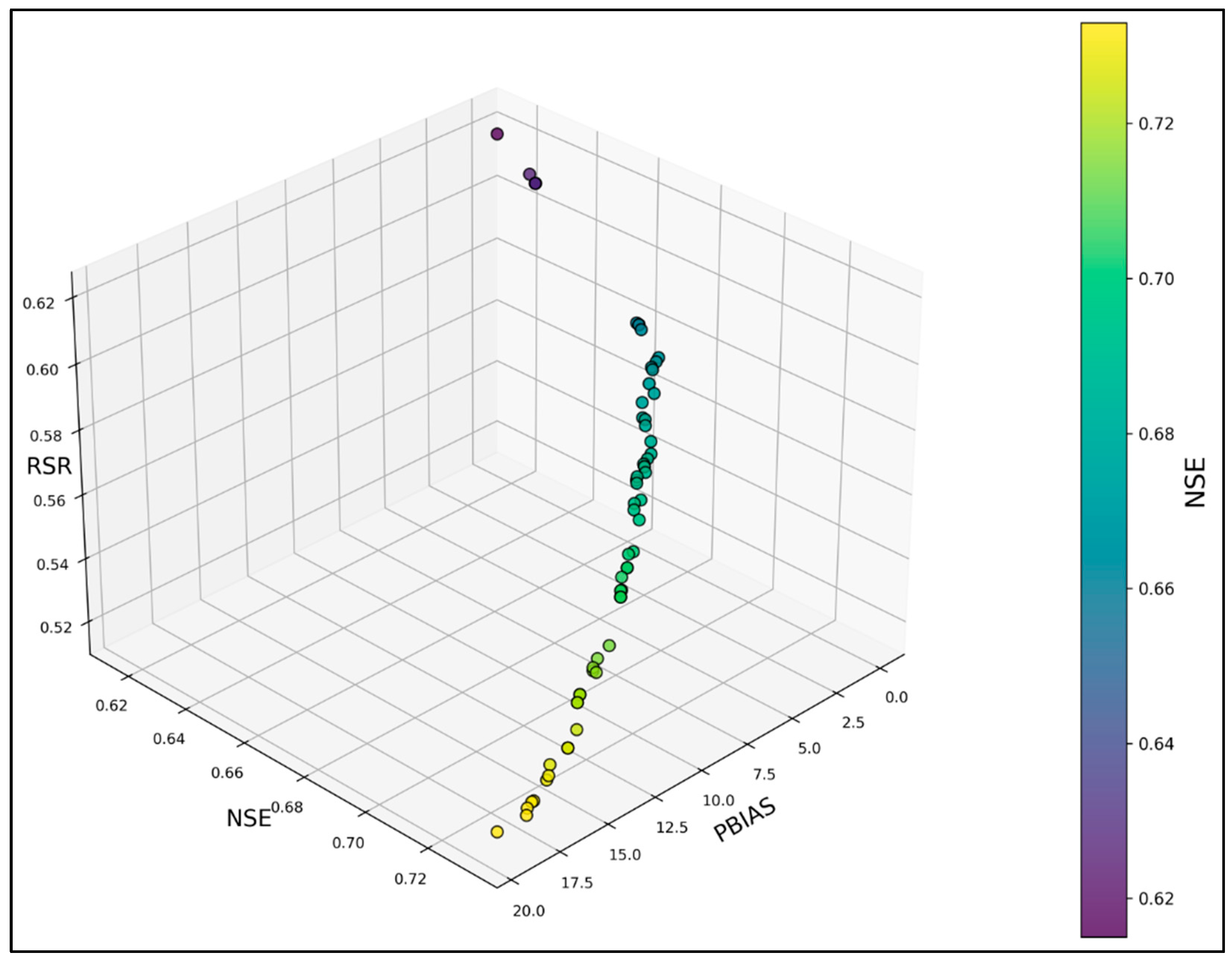
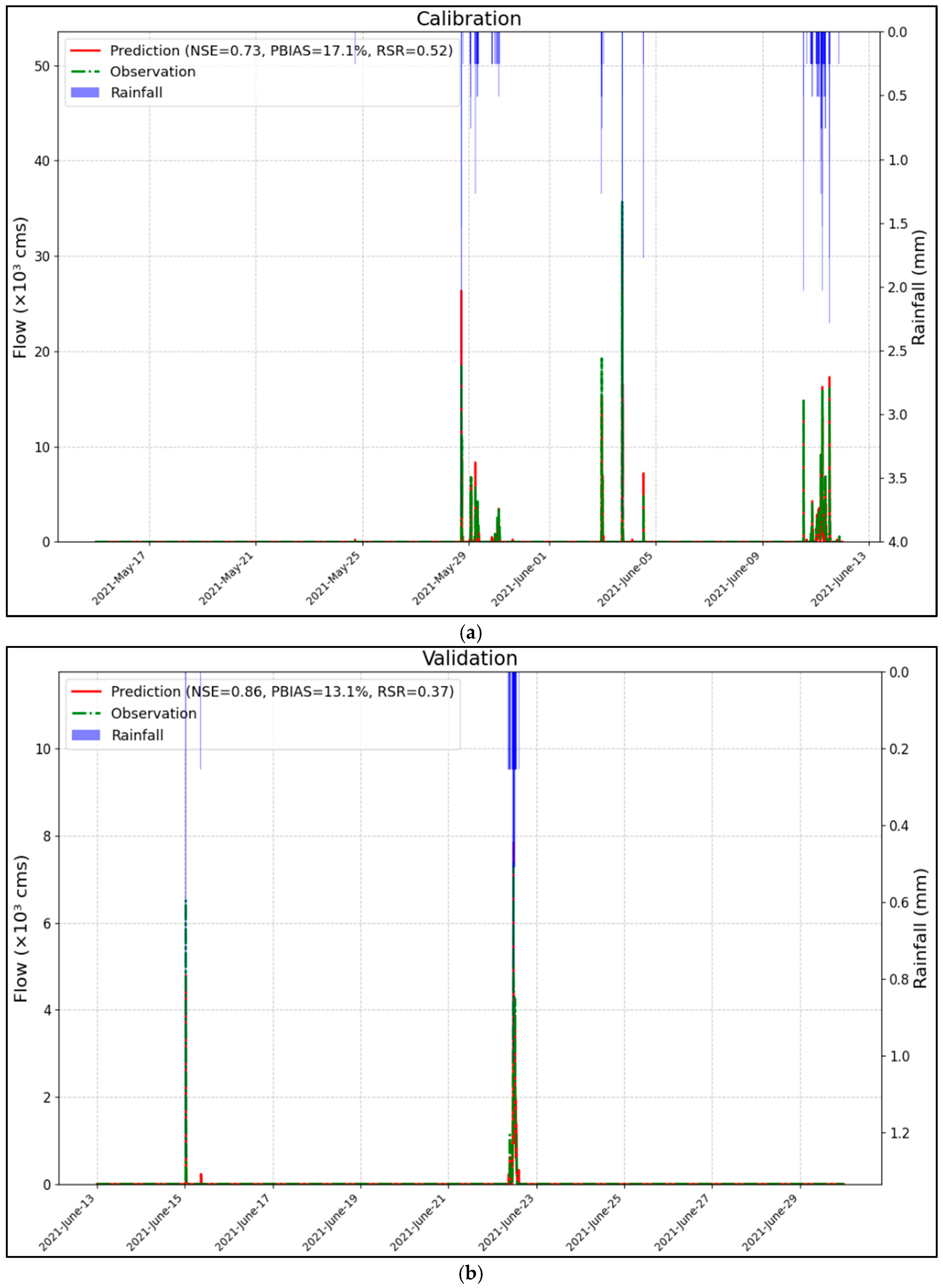
For multi-objective optimization, the NSGA-II algorithm was employed to calibrate the SWMM model, focusing on three objectives: NSE, PBIAS, and RSR. These objectives were used to calibrate a subcatchment within a larger sewershed. The NSE, PBIAS, and RSR values obtained for the calibration period were 0.73, 17.1, and 0.52, respectively, while for the validation period, they were 0.86, 13.1, and 0.37. These results demonstrated the model’s capability to effectively calibrate the SWMM model.

While the developed tool demonstrates strong potential for automating SWMM calibration, several limitations should be acknowledged. The sensitivity analysis relied on OAT method, which does not capture interactions between parameters and may limit comprehensive understanding of parameter influence. Additionally, the calibration was based on a relatively short monitoring period due to data availability. Future research should explore the use of global sensitivity analysis methods to better quantify parameter interactions, extend the tool to support stormwater quality calibration, and investigate hybrid or adaptive optimization strategies to enhance performance across a wider range of hydrologic and watershed conditions.

Overall, the results indicate that this tool is particularly well-suited for calibrating storm runoff simulations in urban sewersheds, where complex drainage networks and spatial variability in hydrologic responses require sophisticated and adaptable modeling approaches. By streamlining and automating the calibration process, the tool helps improve model accuracy and efficiency, supporting better-informed decisions in urban stormwater planning and management. Overall, it offers a practical and extensible framework for developing and applying more robust models in urban stormwater systems.

References

1. Hou, Y.; Kuang, W.; Dou, Y. Observing the compact trend of urban expansion patterns in global 33 megacities during 2000–2020. J. Geogr. Sci. 2023, 33, 2359–2376. [Google Scholar] [CrossRef]
2. Hussain, S.N.; Zwain, H.M.; Nile, B.K. Modeling the effects of land-use and climate change on the performance of stormwater sewer system using SWMM simulation: Case study. J. Water Clim. Change 2022, 13, 125–138. [Google Scholar] [CrossRef]
3. Iffland, R.; Förster, K.; Westerholt, D.; Pesci, M.H.; Lösken, G. Robust vegetation parameterization for green roofs in the EPA stormwater management model (SWMM). Hydrology 2020, 8, 12. [Google Scholar] [CrossRef]
4. Aghakouchak, A.; Jiang, S.C.; Sanders, B.F.; Levin, L.A.; Taylor, S.; Grant, S.B. From rain tanks to catchments: Use of low-impact development to address hydrologic symptoms of the urban stream syndrome. Environ. Sci. Technol. 2015, 49, 11264–11280. [Google Scholar]
5. Luo, K.; Hu, X.; He, Q.; Wu, Z.; Cheng, H.; Hu, Z.; Mazumder, A. Impacts of rapid urbanization on the water quality and macroinvertebrate communities of streams: A case study in Liangjiang New Area. China. Sci. Total Environ. 2018, 621, 1601–1614. [Google Scholar] [CrossRef]
6. Kumar, S.; Guntu, R.K.; Agarwal, A.; Villuri, V.G.K.; Pasupuleti, S.; Kaushal, D.R.; Gosian, A.K.; Bronstert, A. Multi-objective optimization for stormwater management by green-roofs and infiltration trenches to reduce urban flooding in central Delhi. J. Hydrol. 2022, 606, 127455. [Google Scholar] [CrossRef]
7. Behrouz, M.S.; Sample, D.J.; Kisila, O.B.; Harrison, M.; Yazdi, M.N.; Garna, R.K. Parameterization of nutrients and sediment build-up/wash-off processes for simulating stormwater quality from specific land uses. J. Environ. Manag. 2024, 358, 120768. [Google Scholar] [CrossRef]
8. Alamdari, N.; Sample, D.J.; Ross, A.C.; Easton, Z.M. Evaluating the impact of climate change on water quality and quantity in an urban watershed using an ensemble approach. Estuaries Coasts 2020, 43, 56–72. [Google Scholar] [CrossRef]
9. Falconer, R.A. Modelling and forecasting processes in urban environments: Particularly in the UK and China. Hydrology 2025, 4, 82. [Google Scholar] [CrossRef]
10. Salvadore, E.; Bronders, J.; Batelaan, O. Hydrological modelling of urbanized catchments: A review and future directions. J. Hydrol. 2015, 529, 62–81. [Google Scholar] [CrossRef]
11. Ye, C.L.; Xu, Z.X.; Lei, X.H.; Chen, Y.; Ding, X.C.; Liang, Y.S. Simulation and analysis of flooding in urban neighborhoods based on SWMM and Infoworks ICM. Water Conserv. 2023, 39, 87–94. [Google Scholar]
12. Rossman, L.A. Storm Water Management Model User’s Manual Version 5.1; US Environmental Protection Agency: Washington, DC, USA, 2015. [Google Scholar]
13. De Paola, F.; Giugni, M.; Pugliese, F. A harmony-based calibration tool for urban drainage systems. In Water Management; Thomas Telford Ltd.: London, UK, 2018; Volume 171, No. 1; pp. 30–41, Proceedings of the Institution of Civil Engineers. [Google Scholar]
14. Perin, R.; Trigatti, M.; Nicolini, M.; Campolo, M.; Goi, D. Automated calibration of the EPA-SWMM model for a small suburban catchment using PEST: A case study. Environ. Monit. Assess. 2020, 192, 374. [Google Scholar] [CrossRef] [PubMed]
15. Wani, O.; Scheidegger, A.; Carbajal, J.P.; Rieckermann, J.; Blumensaat, F. Parameter estimation of hydrologic models using a likelihood function for censored and binary observations. Water Res. 2017, 121, 290–301. [Google Scholar] [CrossRef]
16. Alamdari, N. Development of a robust automated tool for calibrating a SWMM watershed model. In Proceedings of the World Environmental and Water Resources Congress, Palm Beach, FL, USA, 22–26 May 2016; pp. 221–228. [Google Scholar]
17. James, W.; Kuch, A. Sensitivity-calibration decision-support tools for continuous SWMM modeling: A fuzzy-logic approach. J. Water Manag. Model. 1998, 6, R200–R209. [Google Scholar] [CrossRef]
18. Dell, T.; Razzaghmanesh, M.; Sharvelle, S.; Arabi, M. Development and application of a SWMM-Based simulation model for municipal scale hydrologic assessments. Water 2021, 13, 1644. [Google Scholar] [CrossRef]
19. Zhong, B.; Wang, Z.; Yang, H.; Xu, H.; Gao, M.; Liang, Q. Parameter optimization of SWMM model using integrated Morris and GLUE methods. Water 2022, 15, 149. [Google Scholar] [CrossRef]
20. Wan, B.; James, W. SWMM calibration using genetic algorithms. In Global Solutions for Urban Drainage; American Society of Civil Engineers: Reston, VA, USA, 2002; pp. 1–14. [Google Scholar]
21. Swathi, V.; Raju, K.S.; Varma, M.R.R.; Veena, S.S. Automatic calibration of SWMM using NSGA-III and the effects of delineation scale on an urban catchment. J. Hydroinformatics 2019, 21, 781–797. [Google Scholar] [CrossRef]
22. Alamdari, N.; Sample, D.J. A multiobjective simulation-optimization tool for assisting in urban watershed restoration planning. J. Clean. Prod. 2019, 213, 251–261. [Google Scholar] [CrossRef]
23. Tiernan, E.D. Developing SWMMCALPY: An Automated, Genetic Approach to Calibrating the Storm Water Management Model. Ph.D. Thesis, The University of Texas at Austin, Austin, TX, USA, 2018. [Google Scholar]
24. Behrouz, M.S.; Zhu, Z.; Matott, L.S.; Rabideau, A.J. A new tool for automatic calibration of the Storm Water Management Model (SWMM). J. Hydrol. 2020, 581, 124436. [Google Scholar] [CrossRef]
25. Tolson, B.A.; Shoemaker, C.A. Dynamically dimensioned search algorithm for computationally efficient watershed model calibration. Water Resour. Res. 2007, 43. [Google Scholar] [CrossRef]
26. Vrugt, J.A.; Robinson, B.A. Improved evolutionary optimization from genetically adaptive multimethod search. Proc. Natl. Acad. Sci. USA 2007, 104, 708–711. [Google Scholar] [CrossRef] [PubMed]
27. U.S. Environmental Protection Agency. Assessment of Surface Water Model Maintenance and Support Status; (EPA/600/R-18/265); Office of Research and Development: Washington, DC, USA, 2018. [Google Scholar]
28. U.S. Environmental Protection Agency. Storm Water Management Model (SWMM). Available online: https://github.com/USEPA/Stormwater-Management-Model (accessed on 1 May 2025).
29. Computational Hydraulics International (CHI). PCSWMM-Urban Drainage Modeling Software. Available online: https://www.pcswmm.com (accessed on 1 May 2025).
30. Innovyze. InfoSWMM-Comprehensive Urban Drainage Modeling Software. Available online: https://innovyze.com/products/stormwater-sewer-flood-modeling/xpswmm (accessed on 1 May 2025).
31. U.S. Environmental Protection Agency. SWMM GUI—Storm Water Management Model Graphical User. Urban Water J. 2019, 16, 68–76. Available online: https://github.com/USEPA/SWMM-GUI/tree/master (accessed on 1 May 2025).
32. Leutnant, D.; Döring, A.; Uhl, M. SWMMR-An R package to interface SWMM. Urban Water J. 2019, 16, 68–76. [Google Scholar] [CrossRef]
33. Tanim, A.H.; Smith-Lewis, C.; Downey, A.R.; Imran, J.; Goharian, E. Bayes_Opt-SWMM: A Gaussian process-based Bayesian optimization tool for real-time flood modeling with SWMM. Environ. Model. Softw. 2024, 179, 106122. [Google Scholar] [CrossRef]
34. McDonnell, B.E.; Ratliff, K.; Tryby, M.E.; Wu, J.J.X.; Mullapudi, A. PySWMM: The python interface to stormwater management model (SWMM). J. Open Source Softw. 2020, 5, 1–3. [Google Scholar] [CrossRef]
35. Gu, L.; Sun, Y.; Gao, C.; She, L. A coupled parameter automation calibration module for urban stormwater modelling. Water 2024, 16, 824. [Google Scholar] [CrossRef]
36. Xue, F.; Tian, J.; Wang, W.; Zhang, Y.; Ali, G. Parameter calibration of SWMM model based on optimization algorithm. Comput. Mater. Contin. 2020, 65, 2189–2199. [Google Scholar] [CrossRef]
37. Kim, S.W.; Kwon, S.H.; Jung, D. Development of a multiobjective automatic parameter-calibration framework for urban drainage systems. Sustainability 2022, 14, 8350. [Google Scholar] [CrossRef]
38. Assaf, M.N.; Manenti, S.; Creaco, E.; Giudicianni, C.; Tamellini, L.; Todeschini, S. New optimization strategies for SWMM modeling of stormwater quality applications in urban area. J. Environ. Manag. 2024, 361, 121244. [Google Scholar] [CrossRef]
39. Wang, T.; Zhang, L.; Zhai, J.; Wang, L.; Zhao, Y.; Liu, K. Automatic calibration of SWMM parameters based on multi-objective optimization model. J. Hydroinformatics 2024, 26, 683–706. [Google Scholar] [CrossRef]
40. Rodriguez, M.; Cavadini, G.B.; Cook, L.M. Do baseline assumptions alter the efficacy of green stormwater infrastructure to reduce combined sewer overflows? Water Res. 2024, 253, 121284. [Google Scholar] [CrossRef] [PubMed]
41. Fang, T.; Ball, J.E. Evaluation of spatially variable control parameters in a complex catchment modelling system: A genetic algorithm application. J. Hydroinformatics 2007, 9, 163–173. [Google Scholar] [CrossRef]
42. Qin, H.P.; Li, Z.X.; Fu, G. The effects of low impact development on urban flooding under different rainfall characteristics. J. Environ. Manag. 2013, 129, 577–585. [Google Scholar] [CrossRef]
43. Ashbolt, S.; Aryal, S.; Petrone, K.; McIntosh, B.S.; Maheepala, S.; Chowdhury, R.; Gardner, T. Can stormwater harvesting restore pre-development flows in urban catchments in South East Queensland? Water Sci. Technol. 2013, 67, 446–451. [Google Scholar] [CrossRef]
44. Krebs, G.; Kokkonen, T.; Valtanen, M.; Setälä, H.; Koivusalo, H. Spatial resolution considerations for urban hydrological modelling. J. Hydrol. 2014, 512, 482–497. [Google Scholar] [CrossRef]
45. Di Pierro, F.; Khu, S.T.; Savić, D. From single-objective to multiple-objective multiple-rainfall events automatic calibration of urban storm water runoff models using genetic algorithms. Water Sci. Technol. 2006, 54, 57–64. [Google Scholar] [CrossRef]
46. Zhao, D.; Chen, J.; Wang, H.; Tong, Q. Application of a sampling based on the combined objectives of parameter identification and uncertainty analysis of an urban rainfall-runoff model. J. Irrig. Drain. Eng. 2013, 139, 66–74. [Google Scholar] [CrossRef]
47. Van der Sterren, M.; Rahman, A.; Ryan, G. Modeling of a lot scale rainwater tank system in XP-SWMM: A case study in Western Sydney, Australia. J. Environ. Manag. 2014, 141, 177–189. [Google Scholar] [CrossRef]
48. Xu, Z.; Xiong, L.; Li, H.; Xu, J.; Cai, X.; Chen, K.; Wu, J. Runoff simulation of two typical urban green land types with the Stormwater Management Model (SWMM): Sensitivity analysis and calibration of runoff parameters. Environ. Monit. Assess. 2019, 191, 1–16. [Google Scholar] [CrossRef]
49. Rosa, D.J.; Clausen, J.C.; Dietz, M.E. Calibration and verification of SWMM for low impact development. JAWRA J. Am. Water Resour. Assoc. 2015, 51, 746–757. [Google Scholar] [CrossRef]
50. Del Giudice, G.; Padulano, R. Sensitivity analysis and calibration of a rainfall-runoff model with the combined use of EPA-SWMM and genetic algorithm. Acta Geophys. 2016, 64, 1755–1778. [Google Scholar] [CrossRef]
51. Krebs, G.; Kokkonen, T.; Valtanen, M.; Koivusalo, H.; Setälä, H. A high resolution application of a stormwater management model (SWMM) using genetic parameter optimization. Urban Water J. 2013, 10, 394–410. [Google Scholar] [CrossRef]
52. Vassiljev, A.; Suits, K.; Kaur, K.; Kändler, N.; Truu, M.; Annus, I. Automatic calibration toolbox for SWMM5. Adv. Eng. Softw. 2023, 185, 103528. [Google Scholar] [CrossRef]
53. Dent, S.; Hanna, R.B.; Wright, L.T. Automated calibration using optimization techniques with SWMM RUNOFF. J. Water Manag. Model. 2004, 2004. 32, 45–52. [Google Scholar] [CrossRef]
54. Blank, J.; Deb, K. Pymoo: Multi-objective optimization in python. IEEE Access 2020, 8, 89497–89509. [Google Scholar] [CrossRef]
55. Li, S.; Wang, Z.; Wu, X.; Zeng, Z.; Shen, P.; Lai, C. A novel spatial optimization approach for the cost-effectiveness improvement of LID practices based on SWMM-FTC. J. Environ. Manag. 2022, 307, 114574. [Google Scholar] [CrossRef]
56. El Kounni, A.; Outzourhit, A.; Mastouri, H.; Radoine, H. Building energy model automated calibration using Pymoo. Energy Build. 2023, 298, 113524. [Google Scholar] [CrossRef]
57. Sample, D.J.; Behrouz, M.S.; Harrison, M.R.; Yazdi, M.N.; Kisila, B.O.; Lanier, J. Runoff Water Quality Monitoring for Total Phosphorus, Total Nitrogen, and Total Suspended Solids in the City of Fredericksburg, VA; Resources Protection Group, 2023; LLC RIVERE; Available online: https://resourceprotectiongroup.org/wp-content/uploads/2023/02/RPG-Fred-Report020323.pdf (accessed on 20 December 2024).
58. Behrouz, M.S.; Ahmadi, H. SWMM Model-City of Fredericksburg; HydroShare: Raleigh, NC, USA, 2024; Available online: https://www.hydroshare.org/resource/2c4a324dbe0d487690b7b79eb0bfd618 (accessed on 20 December 2024).
59. Virginia Geographic Information Network (VGIN). Virginia LiDAR Inventory Web Mapping Application. 2021. Available online: https://vgin.vdem.virginia.gov/apps/VGIN::virginia-lidar-download-application/explore (accessed on 1 January 2022).
60. NOAA’s National Climatic Data Center (NCDC). National Oceanic and Atmospheric Administration. 2020. Available online: https://www.ncdc.noaa.gov/ (accessed on 11 January 2020).
61. Green, W.H.; Ampt, G.A. Studies on Soil Physics. J. Agric. Sci. 1911, 4, 1–24. [Google Scholar] [CrossRef]
62. U.S. Department of Agriculture Natural Resources Conservation Service. Web Soil Survey Geographic Database (SSURGO); U.S. Department of Agriculture: Washington, DC, USA, 2021. [Google Scholar]
63. Yazdi, M.N.; Ketabchy, M.; Sample, D.J.; Scott, D.; Liao, H. An evaluation of HSPF and SWMM for simulating streamflow regimes in an urban watershed. Environ. Model. Softw. 2019, 118, 211–225. [Google Scholar] [CrossRef]
64. Fredericksburg and Spotsylvania County Battlefields Memorial National Military Park. Geologic Resources Inventory Report, Natural Resource Report NPS/NRPC/GRD/NRR—2010/229; Natural Resource Program Center: Denver, CO, USA, 2010. [Google Scholar]
65. Moriasi, D.N.; Arnold, J.G.; Van Liew, M.W.; Bingner, R.L.; Harmel, R.D.; Veith, T.L. Model evaluation guidelines for systematic quantification of accuracy in watershed simulations. Trans. ASABE 2007, 50, 885–900. [Google Scholar] [CrossRef]
66. Ballinas-González, H.A.; Alcocer-Yamanaka, V.H.; Canto-Rios, J.J.; Simuta-Champo, R. Sensitivity analysis of the rainfall–runoff modeling parameters in data-scarce urban catchment. Hydrology 2020, 7, 73. [Google Scholar] [CrossRef]
67. Niazi, M.; Nietch, C.; Maghrebi, M.; Jackson, N.; Bennett, B.R.; Tryby, M.; Massoudieh, A. Storm water management model: Performance review and gap analysis. J. Sustain. Water Built Environ. 2017, 3, 04017002. [Google Scholar] [CrossRef] [PubMed]
68. James, W.R.C.; Wan, B.; James, W. Implementation in PCSWMM using genetic algorithms for auto calibration and design-optimization. In Global Solutions Urban Drainage; American Society of Civil Engineers: Reston, VA, USA, 2002; pp. 1–10. [Google Scholar]
69. Behrouz, M.S.; Sample, D.J.; Yazdi, M.N. Robustness of storm water management model parameter sets for dry and wet hydroclimatic conditions. J. Clean. Prod. 2023, 411, 137328. [Google Scholar] [CrossRef]
70. Barco, J.; Wong, K.M.; Stenstrom, M.K. Automatic calibration of the US EPA SWMM model for a large urban catchment. J. Hydraul. Eng. 2008, 134, 466–474. [Google Scholar] [CrossRef]
Figure 1. PYSWMM-PYMOO linkage.
Hydrology 12 00129 g001
Figure 2. Maps display (a) the geographic location of Fredericksburg, VA, and (b) the delineated sewershed boundary.
Hydrology 12 00129 g002aHydrology 12 00129 g002b
Figure 3. Land use map of City of Fredericksburg.
Hydrology 12 00129 g003
Figure 4. Monitoring locations used for model calibration.
Hydrology 12 00129 g004
Figure 5. Sensitivity analysis of 15 selected parameters with respect to (a) total flow volume (b) peak flow.
Hydrology 12 00129 g005aHydrology 12 00129 g005b
Figure 6. The SWMM model of entire catchment.
Hydrology 12 00129 g006
Figure 7. The subset of subcatchments within the sewershed.
Hydrology 12 00129 g007
Figure 8. Convergence of single objective optimization.
Hydrology 12 00129 g008
Figure 9. Comparison between the observed and simulated flow (a) calibration and (b) validation periods for single objective calibration.
Hydrology 12 00129 g009
Figure 10. Commercial subcatchment for multi-objective calibration.
Hydrology 12 00129 g010
Figure 11. Pareto front in multi-objective calibration.
Hydrology 12 00129 g011
Figure 12. Comparison between the observed and simulated flow: (a) calibration and (b) validation periods for multi-objective calibration.
Hydrology 12 00129 g012