Triangular Fuzzy Finite Element Solution for Drought Flow of Horizontal Unconfined Aquifers

Abstract

In this paper, a novel approximate triangular fuzzy finite element method (FEM) is proposed to solve the one-dimensional second-order unsteady nonlinear fuzzy partial differential Boussinesq equation. The physical problem concerns the case of the drought flow of a horizontal unconfined aquifer with a limited breath B and special boundary conditions: (a) at x = 0, the water level is equal to zero, and (b) at x = B, the flow rate is equal to zero due to the presence of an impermeable wall. The initial water table is assumed to be curvilinear, following the form of an inverse incomplete beta function. To account for uncertainties in the system, the hydraulic parameters—hydraulic conductivity (K) and porosity (S)—are treated as fuzzy variables, considering sources of imprecision such as measurement errors and human-induced uncertainties. The performance of the proposed fuzzy FEM scheme is compared with the previously developed orthogonal fuzzy FEM solution as well as with an analytical solution. The results are in close agreement with those of the other methods, with the mean error of the analytical solution found to be equal to $1.19·{10}^{-6}$. Furthermore, the possibility theory is applied and fuzzy estimators constructed, leading to strong probabilistic interpretations. These findings provide valuable insights into the hydraulic properties of unconfined aquifers, aiding engineers and water resource managers in making informed and efficient decisions for sustainable hydrological and environmental planning.

1. Introduction

The drought flow in a river system can be described as the drainage flow from the groundwater aquifers in the basin. Practically, it is the rate of flow that a given catchment can supply in the absence of precipitation and in the absence of artificial storage works. It is often referred to as groundwater recession flow, base flow, low flow, percolation flow, and sustained flow.

Many authors have discussed particular aspects of base flow, and between them, Hall (1968) [1] described a complete review of existing solutions until 1967. According to him, the basic differential equation governing flow in an aquifer was presented by Boussinesq in 1877. Boussinesq linearized the nonlinear equation by making simplifying assumptions, and the result was a form of the heat flow or diffusion equation that can be solved more readily. Boussinesq, in 1904 [2], further developed his solution, introducing a non nonlinear solution with the assumption that a stream is located on a horizontal, impermeable lower boundary with an initial curvilinear water table and zero water-level elevation in the stream. Brutsaert and Nieber (1977) [3] examined the drought or base flow characteristics of six basins in the Finger Lakes region. They concluded that among several expressions, Boussinesq’s nonlinear solution of free surface groundwater flow is best suited to parameterize the observed hydrographs. Troch et al. (1993) [4] have used Boussinesq’s solution in order to estimate the catchment-scale parameters, namely, the aquifer hydraulic conductivity and the average depth to the impervious layer. Szilagyi et al. (1998) [5] have tested the recession flow analysis of Brutsaert and Nieber (1977) [3] and Troch et al. (1993) [4] using a numerical model. They have found that the estimation of the catchment-scale saturated hydraulic conductivity and mean aquifer depth were reliable. Troch et al. (2004) [6] presented an analytical solution, providing analytical solutions to storage-based subsurface flow equations in catchment studies. Based on a literature overview, Troch et al. (2013) [7] summarize the impact and legacy of the contributions of Wilfried Brutsaert and Jean-Yves Parlange concerning many applications in catchment hydrology, ranging from drought flow analysis to surface water–groundwater interactions. An exact solution to the full nonlinear Boussinesq equation is presented by Bartlett and Porporato (2018) [8], and their solution applies to sloping aquifers and accounts for source and sink terms such as bedrock seepage, an often-significant flux in headwater catchments. This new solution provides a more realistic representation of streamflow and groundwater dynamics in hillslopes. Conceptual approximations of the Boussinesq equation were introduced and analyzed by Akylas and Gravanis (2024) [9], resulting in a very accurate and well-applicable model for horizontal unconfined aquifers during the pure drainage phase, without any recharge and zero-inflow conditions.

Many numerical solutions to the problem of the water response to recharge or discharge of an aquifer have been developed in the past. Among the various numerical methods, the most commonly used techniques are the finite difference method (FDM), finite volume method (FVM), and finite element method (FEM). The FDM is a well-established and simple method, approximating the governing equations [10]. Although many fluid dynamics problems may be solved using the FDM, as soon as irregular geometries are encountered, the FDM technique becomes difficult to use. The FVM is a further refined version of the FDM and has become popular in computational fluid dynamics [11]. There is a similarity between the FVM technique and the linear FEM. The FEM method is a numerical tool for determining approximate solutions to a large class of engineering problems. The FEM considers that the solution region comprises many small, interconnected sub-regions or elements, approximating the governing equations, and reduces the complex partial differential equations to either linear or nonlinear simultaneous equations. Also, this method allows a close representation of the boundaries of complicated domains [12,13,14].

Therefore, the FEM is a popular method for numerically solving partial differential equations arising in engineering and mathematical modeling, including traditional fields of structural analysis, heat transfer, fluid flow, mass transport, and electromagnetic potential. According to Oden (1990) [15], “no other family of approximation methods has had a greater impact on the theory and practice of numerical methods during the twentieth century”. Many numerical solutions based on FEM methods concerning hydraulic problems have been presented. Tzimopoulos (1976) [16] studied a physical problem of a free surface flow toward a ditch or a river. The solution to Boussinesq’s equation was made by the application of the FEM. Galerkin’s method [17] was used, leading to a system of nonlinear equations. Numerical results were compared with the exact solution of Boussinesq and with other FDM approximations. Frangakis and Tzimopoulos (1979) [18] investigated a numerical model based on Boussinesq’s equation describing the unsteady groundwater flow on impervious sloping bedrock. The numerical model uses the FEM technique with Galerkin’s method. The stability and accuracy of the method have been proved by the comparison of numerical results with the Crank–Nicolson scheme. Tzimopoulos and Tolikas (1980) [19] investigated the problem of artificial groundwater recharge in the case of an unconfined aquifer, described by the Boussinesq equation. The problem was solved by analytical and numerical methods, and the FEM method was used with square elements. Tber and Talibi (2007) [20] presented a numerical method of FEM to automatically identify hydraulic conductivity in the seawater intrusion problem when a sharp interface approach is used. Mohammadnejad and Khoei (2013) [21] presented a fully coupled numerical model developed for the modelling of the hydraulic fracture propagation in porous media using the extended FEM method in conjunction with the cohesive crack model. Yang et al. (2019) [22] proposed a novel computational methodology to simulate the nonlinear hydro-mechanical process in saturated porous media containing crossing fractures. The nonlinear hydro-mechanical coupled equations are obtained by Extended Finite Element Method (XFEM) discretization and solved by the Newton–Raphson method. Aslan and Temel (2022) [23] described the 2D steady-state seepage analysis of the dam body and its base investigated using the FEM based on Galerkin’s approach. The body and foundation soil are considered as homogeneous isotropic and anisotropic materials, and the effects of horizontal drainage length and the cutoff wall on seepage are investigated.

Since the aforementioned problem concerns differential equations, which present particular problems regarding fuzzy logic, a significant number of research studies were carried out in that field, especially regarding the fuzzy differentiation of functions. Initially, fuzzy differentiable functions were studied by Puri and Ralescu (1983) [24], who generalized and extended Hukuhara’s fundamental study [25] (H-derivative) of a set of values appearing in fuzzy sets. Kaleva (1987) [26] and Seikkala (1987) [27] developed a theory on fuzzy differential equations. In the last few years, several studies have been carried out in the theoretical and applied research fields on fuzzy differential equations with an H-derivative [26,28,29]. Nevertheless, in many cases, this method has presented certain drawbacks, since it has led to solutions with increasing support, along with increasing time [30]. This proves that, in some cases, this solution is not a representative generalization of the classic case. To overcome this drawback, the generalized derivative gH (gH-derivative) was introduced [31,32,33,34]. The gH-derivative will be used henceforth for a more extensive degree of fuzzy functions than the Hukuhara derivative.

In the current work, the solution of the one-dimensional second-order unsteady nonlinear fuzzy partial differential Boussinesq equation is examined. The physical problem concerns the case of drought flow of a horizontal unconfined aquifer with a limited breath B and special boundary conditions: at x = 0, the water level is equal to zero, and at x = B, the flow rate is equal to zero because of the existence of an impermeable wall. Additionally, the water table is initially curvilinear in the form of an inverse incomplete beta function. The hydraulic parameters (hydraulic conductivity, K, and porosity, S) of the physical problem are considered fuzzy for various reasons (e.g., machine impression, human errors, etc.). This problem is encountered with a new triangular fuzzy FEM numerical solution, and Galerkin method is used, leading to a system of crisp boundary value problems. Thus, the main novelty and goals of this work were threefold, as follows: (1) to develop a new fuzzy FEM numerical scheme based on triangular elements; (2) to define the range where the analytical solutions approximate the new FEM numerical solution as well as to make a comparative analysis between the new triangular fuzzy FEM solution, the analytical solution, and the previous developed orthogonal fuzzy FEM solution [35]; and (3) to apply the possibility theory to the fuzzy estimators, leading to strong probability solutions for some hydraulic entities, which help the engineers and designers of water resource projects, gaining knowledge of hydraulic properties and taking the right decision for rational and productive engineering studies.

2. Materials and Methods

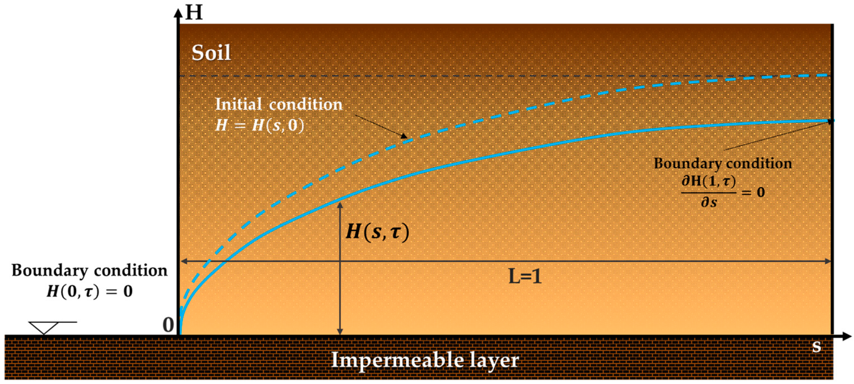
2.1. Crisp Model

As mentioned in the Introduction for the case of one-dimensional horizontal flow, the Boussinesq equation describing recession flow is

$${\displaystyle \frac{\mathsf{\partial }h}{\mathsf{\partial }t}}={\displaystyle \frac{K}{S}}{\displaystyle \frac{\mathsf{\partial }}{\mathsf{\partial }x}}\left(h{\displaystyle \frac{\mathsf{\partial }h}{\mathsf{\partial }x}}\right)$$

(1)

Figure 1 provides the definition sketch of the investigated physical problem.

The initial and boundaries conditions are

$$\begin{gathered} t=0, h(x,0)=h\left(x\right), \\ t>0, h\left(0,t\right)=0, {\displaystyle \frac{\mathsf{\partial }h(L,t)}{\mathsf{\partial }x}}=0 \end{gathered}$$

(2)

We introduce now non-dimensional variables, as follows:

$$H={\displaystyle \frac{h}{h_0}}, s={\displaystyle \frac{x}{L}}, \tau ={\displaystyle \frac{K{h}_{0}t}{2S{L}^2}}$$

(3)

The Boussinesq equation becomes

$${\displaystyle \frac{\mathsf{\partial }H}{\mathsf{\partial }\tau }}={\displaystyle \frac{\mathsf{\partial }}{\mathsf{\partial }s}}\left(2H{\displaystyle \frac{\mathsf{\partial }H}{\mathsf{\partial }s}}\right),$$

(4)

with the new initial and boundary conditions

$$\begin{array}{l}\tau =0, H(s,0)=H\left(s\right),\\ \tau >0, H\left(0,\tau \right)=0, {\displaystyle \frac{\mathsf{\partial }\left(H\right(1,\tau \left)\right)}{\mathsf{\partial }s}}=0\end{array}$$

(5)

where $\left(h\left(x\right), H\left(s\right)\right)$ is the initial water table of the aquifer.

Numerical Method

For the solution of Equation (4), the FEM method has been used. The domain of integration (s, τ) is divided into triangular elements with dimensions Δs and Δτ/2. The global nodal points are numbered with large numbers 1, 2, …, G, while the local ones inside each element are numbered with small letters (i, j, k) (Figure 2b). Equation (4) is nonlinear, and thus the more suitable numerical method for the construction of a model with finite elements is Galerkin’s method [14].

Using this method, Equation (4) is written as follows:

$$L(\overline{H})={\displaystyle \frac{\mathsf{\partial }\overline{H}}{\mathsf{\partial }\tau }}-{\displaystyle \frac{\mathsf{\partial }}{\mathsf{\partial }s}}\left(2\overline{H}{\displaystyle \frac{\mathsf{\partial }\overline{H}}{\mathsf{\partial }s}}\right)=r_0,$$

(6)

where $r_0$ = a small quantity and $\overline{H}$ = an approximating function to H.

In Galerkin’s method, the global basis function ${\Phi }_{\Delta }\left(\overrightarrow{X}\right)$ (Figure 2a) is orthogonal with respect to the operator $L\left(\overline{H}\right)$, that is,

$${\int }_{R}L\left(\overline{H}\right){\Phi }_{\Delta }\left(\overrightarrow{X}\right)dR=0, \overrightarrow{X}=\left(s,\tau \right), \Delta =\mathrm{1,2},\dots ,G.$$

(7)

(Note: henceforth, we skip the over line in H for practical reasons).

Using Green’s theorem, Equation (7) gives the following nonlinear algebraic equation (see also Appendix A):

$$\begin{array}{c}{\displaystyle \frac{\lambda }{2}}(\Delta H^2{)}_i^{j+1/2}-{\displaystyle \frac{(H_i^{j+1}-H_i^j)}{3}}-{\displaystyle \frac{(H_{i-1}^{j+1}-H_{i-1}^j)}{12}}-{\displaystyle \frac{(H_{i+1}^{j+1/2}-H_{i+1}^j)}{12}}=0=\\ {\displaystyle \frac{\lambda }{4}}\{(\Delta H^2{)}_i^{j+1}+(\Delta H^2{)}_i^j\}-{\displaystyle \frac{(H_i^{j+1}-H_i^j)}{3}}-{\displaystyle \frac{(H_{i-1}^{j+1}-H_{i-1}^j)}{12}}-{\displaystyle \frac{(H_{i+1}^{j+1/2}-H_{i+1}^j)}{12}}\\ i=\mathrm{1,2}, \dots \dots ,nj=\mathrm{1,2}, \dots \dots ,k\end{array}$$

(8)

where λ = Δt/Δs² and the operator $(\Delta H^2{)}_i^j=(H^2{)}_{i+1}^j-2(H^2{)}_i^j+(H^2{)}_{i-1}^j$. The nonlinear terms are linearized by taking the following form:

$$\begin{array}{c}(H^2{)}_{i-1}^{j+1}=(H^2{)}_{i-1}^j+{\displaystyle \frac{\mathsf{\partial }\left(H^2\right)}{\mathsf{\partial }H}}(H_{i-1}^{j+1}-H_{i-1}^j)=2H_{i-1}^j{H}_{i-1}^{j+1}-(H^2{)}_{i-1}^j\\ -2(H^2{)}_i^{j+1}=-2(H^2{)}_i^j-2{\displaystyle \frac{\mathsf{\partial }\left(H^2\right)}{\mathsf{\partial }H}}(H_i^{j+1}-H_i^j)=-4H_i^j{H}_i^{j+1}+2(H^2{)}_i^j\\ (H^2{)}_{i+1}^{j+1}=(H^2{)}_{i+1}^j+{\displaystyle \frac{\mathsf{\partial }\left(H^2\right)}{\mathsf{\partial }H}}(H_{i-1}^{j+1}-H_{i-1}^j)=2H_{i+1}^j{H}_{i+1}^{j+1}-(H^2{)}_{i+1}^j\end{array}$$

(9)

The functions at the point (i, j + 1/2) are approximated by

$$(H^2{)}_{\mathrm{i},\mathrm{j}+1/2}={\displaystyle \frac{1}{2}}((H^2{)}_{\mathrm{i},\mathrm{j}}+(H^2{)}_{\mathrm{i},\mathrm{j}+1})$$

(10)

Under the above simplifications, the linearized equation becomes

$$\begin{array}{c}{A}_i{X}_{i-1}+B_i{X}_i+C_i{X}_{i+1}=D_i\\ A_i=({\displaystyle \frac{1}{4}}-1.5\lambda H_{i-1}^j),B_i=(3\lambda H_i^j+1),C_i=({\displaystyle \frac{1}{4}}-1.5\lambda H_{i+1}^j),\\ D_i={\displaystyle \frac{1}{4}}(H_{i-1}^j+4H_i^j+H_{i+1}^j)\\ X_{i-1}\equiv H_{i-1}^{j+1},X_i\equiv H_i^{j+1},X_{i+1}\equiv H_{i+1}^{j+1}\end{array}$$

(11)

The solution of Equation (11) could be obtained by the well-known Thomas algorithm [36] for tridiagonal systems, while newer efficient explicit inverse formulas [37] can also be used.

2.2. Fuzzy Model Definitions

To facilitate the understanding of readers non-familiar with fuzzy and possibility theory, in the subsections below, several necessary definitions will be provided, concerning some preliminaries in fuzzy theory [38] and some definitions about the differentiability and possibility theory.

2.2.1. Fuzzy Theory Definitions

Definition 1. 

A fuzzy set $\tilde{U}$ on a universe set X is a mapping $\tilde{U}:X\to \left[\mathrm{0,1}\right]$, assigning to each element $x\in X$ a degree of membership $0\le \tilde{U}\left(x\right)\le 1.$ The membership function is also defined as ${\mu }_{\tilde{U}}\left(x\right)$ with the following properties: (i) ${\mu }_{\tilde{U}}$ is upper semicontinuous; (ii) ${\mu }_{\tilde{U}}\left(x\right)$ = 0 outside of some interval [c, d]; (iii) there are real numbers $c\le a\le b\le d$, such that ${\mu }_{\tilde{U}}$ is increasing on [c, a], decreasing on [b, d], and ${\mu }_{\tilde{U}}\left(x\right)$ = 1 for each $x\in [a,b]$; and (iv) $\tilde{U}$ is a convex fuzzy set, i.e.,

$${\mu }_{\tilde{U}}(\lambda x+(1-\lambda \left)x\right)\ge \mathit{min}\{{\mu }_{\tilde{U}}\left(\lambda x\right),{\mu }_{\tilde{U}}\left(\right(1-\lambda \left)x\right)\}$$

Definition 2. 

Let X be a Banach space and $\tilde{U}$ be a fuzzy set on X. The α-cuts of $\tilde{U}$ are defined as $[\tilde{U}{]}_{\alpha }=\{x\in R\left|\tilde{U}\left(x\right)\ge \alpha \right.\},\alpha \in (\mathrm{0,1}]$ and for α = 0 the closure is

$$[\tilde{U}{]}_0=\stackrel{------------------}{\{x\in R\left|\tilde{U}\left(x\right)>0\right.\}}$$

Definition 3. 

Let Ҡ(X) be the family of all nonempty compact convex subsets of a Banach space. A fuzzy set $\tilde{U}$ on X is called compact if $[\tilde{U}{]}_{\alpha }\in$ Ҡ(X), $\forall \alpha \in \left[\mathrm{0,1}\right].$ The space of all compact and convex fuzzy sets on X is denoted as Ƒ (X).

Definition 4. 

Let $\tilde{U}\in$ Ƒ (R). The α-cuts of $\tilde{U}$, are $[\tilde{U}{]}_{\alpha }=[U_{\alpha }^{-},U_{\alpha }^{+}]={\Delta }_{\alpha }$. According to the representation theorem of Negoita and Ralescu (1975) [39] and the theorem of Goetschel and Voxman (1986) [40], the membership function and the α-cut form of a fuzzy number $\tilde{U}$ are equivalent, and, in particular, the α-cuts $[\tilde{U}{]}_{\alpha }=[U_{\alpha }^{-},U_{\alpha }^{+}]={\Delta }_{\alpha }$ uniquely represent $\tilde{U}$, provided that the two functions are monotonic ($U_{\alpha }^{-}$ increasing, $U_{\alpha }^{+}$ decreasing) and $U_1^{-}\le U_1^{+}, for \alpha =1.$

Definition 5. 

gH-Differentiability [41]. Let $\tilde{U}:[a,b] \to$ Ƒ (R) be such that $\left[\tilde{U}\right(x){]}_{\alpha }=[U_{\alpha }^{-}\left(x\right),U_{\alpha }^{+}\left(x\right)]={\Delta }_{\alpha }$. Suppose that the functions $U_{\alpha }^{-}\left(x\right)$, $U_{\alpha }^{+}\left(x\right)$ are real-valued functions, differentiable with respect to x and uniform with respect to $\alpha \in \left[\mathrm{0,1}\right]$. Then, the function $\tilde{U}\left(x\right)$ is gH-differentiable at a fixed $x\in [a,b]$ if and only if one of the following two cases holds:

(a)

${\left(U_{\alpha }^{-}\right)}^{\prime }\left(x\right)$ is increasing, ${\left(U_{\alpha }^{+}\right)}^{\prime }\left(x\right)$ is decreasing as functions of α, and ${\left(U_{\alpha }^{-}\right)}^{\prime }\left(x\right)\le {\left(U_{\alpha }^{+}\right)}^{\prime }\left(x\right)]$;

(b)

${\left(U_{\alpha }^{-}\right)}^{\prime }\left(x\right)$ is decreasing, ${\left(U_{\alpha }^{+}\right)}^{\prime }\left(x\right)$ is increasing as functions of α, and ${\left(U_{\alpha }^{+}\right)}^{\prime }\left(x\right)\le {\left(U_{\alpha }^{-}\right)}^{\prime }\left(x\right)]$.

Note: ${\left(U_{\alpha }^{-}\right)}^{\prime }(x)={\displaystyle \frac{d{U}_{\alpha }^{-}(x)}{dx}},{\left(U_{\alpha }^{+}\right)}^{\prime }(x)={\displaystyle \frac{d{U}_{\alpha }^{+}\left(x\right)}{dx}}$. In both of the above cases, the ${\tilde{U}}_{\alpha }^{\prime }\left(x\right)$ derivative is a fuzzy number.

Definition 6. 

gH-differentiable at $x_0$. Let $\tilde{U}:[a,b]\to$ Ƒ(R) and $x_0\in [a,b]$ with $U_{\alpha }^{-}\left(x\right)$, $U_{\alpha }^{+}\left(x\right)$ both be differentiable at $x_0$. According to [41] it is

• $\tilde{U}$ is (i)-gH-differentiable at $x_0$ if

  (i)

  ${\left[{\tilde{U}}_{gH}^{\prime }\left(x_0\right)\right]}_a=\left[{\left(U_{\alpha }^{-}\right)}^{\prime }\left(x_0\right),{\left(U_{\alpha }^{+}\right)}^{\prime }\left(x_0\right)\right], \forall \alpha \in \left[\mathrm{0,1}\right]$;

• $\tilde{U}$ is (ii)-gH-differentiable at $x_0$ if

  (i)

  ${\left[{\tilde{U}}_{gH}^{\prime }\left(x_0\right)\right]}_a=\left[{\left(U_{\alpha }^{+}\right)}^{\prime }\left(x_0\right),{\left(U_{\alpha }^{-}\right)}^{\prime }\left(x_0\right)\right], \forall \alpha \in \left[\mathrm{0,1}\right]$.

Definition 7. 

g-differentiability. Let $\tilde{U}:[a,b]\to$ Ƒ(R) be such that $\left[\tilde{U}\right(x){]}_{\alpha }=[U_{\alpha }^{-}\left(x\right),U_{\alpha }^{+}\left(x\right)]$. If $U_{\alpha }^{-}\left(x\right)$ and $U_{\alpha }^{+}\left(x\right)$ are differentiable real-valued functions with respect to x and uniform for $\alpha \in \left[\mathrm{0,1}\right]$, then ${\tilde{U}}_{\alpha }\left(x\right)$ is g-differentiable and it is valid that [41]

$${\left[{\tilde{U}}_g^{\prime }\left(x\right)\right]}_a=\left[\underset{\beta \ge \alpha }{inf}\mathit{min}\{(U_{\alpha }^{-}{)}^{\prime }(x),(U_{\alpha }^{+}{)}^{\prime }(x)\},\underset{\beta \ge \alpha }{sup}\mathit{max}\{(U_{\alpha }^{-}{)}^{\prime }(x),(U_{\alpha }^{+}{)}^{\prime }(x)\}\right]$$

Definition 8. 

The gH-differentiability implies g-differentiability, but the inverse is not true.

Definition 9. 

[gH-p] differentiability. A fuzzy-valued function $\tilde{U}$ of two variables is a rule that assigns to each ordered pair of real numbers (x, t) in a set D, a unique fuzzy number denoted by $\tilde{U}(x,t)$. Let $\tilde{U}(x,t)$: D $\to$ R_Ƒ, (x₀, t₀)$\in$ D and $U_{\alpha }^{-}(x,t)$, $U_{\alpha }^{+}(x,t)$ be real-valued functions and partially differentiable with respect to x. According to [34,42] it is

• $\tilde{U}(x,t)$ is [(i)-p]-differentiable with respect to x at ($x_0, t_0)$ if

  $${\displaystyle \frac{\mathsf{\partial }{\tilde{U}}_{\alpha }(x_0,t_0)}{\mathsf{\partial }{x}_{i.gH}}}=[{\displaystyle \frac{\mathsf{\partial }{U}_{\alpha }^{-}(x_0,t_0)}{\mathsf{\partial }x}},{\displaystyle \frac{\mathsf{\partial }{U}_{\alpha }^{+}(x_0,t_0)}{\mathsf{\partial }x}}]$$
• $\tilde{U}(x,t)$ is [(ii)-p]-differentiable with respect to x at ($x_0, t_0)$ if

  $${\displaystyle \frac{\mathsf{\partial }{\tilde{U}}_{\alpha }(x_0,t_0)}{\mathsf{\partial }{x}_{ii.gH}}}=[{\displaystyle \frac{\mathsf{\partial }{U}_{\alpha }^{+}(x_0,t_0)}{\mathsf{\partial }x}},{\displaystyle \frac{\mathsf{\partial }{U}_{\alpha }^{-}(x_0,t_0)}{\mathsf{\partial }x}}]$$

Definition 10. 

Let $\tilde{U}(x,t)$: D $\to$ Ƒ (R), and ${\displaystyle \frac{\mathsf{\partial }{\tilde{U}}_{\alpha }(x_0,t_0)}{\mathsf{\partial }{x}_{i.gH}}}$ be [gH-p]-differentiable at ($x_0, t_0)$ $\in$ D with respect to x. It is valid that [34,42]

• ${\displaystyle \frac{\mathsf{\partial }{\tilde{U}}_{\alpha }(x_0,t_0)}{\mathsf{\partial }{x}_{i.gH}}}$ is [(i)-p]-differentiable with respect to x if

$${\displaystyle \frac{{\mathsf{\partial }}^2{\tilde{U}}_{\alpha }(x_0,t_0)}{\mathsf{\partial }{x^2}_{i.gH}}}=\left\{\begin{array}{c}\left[{\displaystyle \frac{{\mathsf{\partial }}^2{U}_{\alpha }^{-}\left(x_0,t_0\right)}{\mathsf{\partial }{x}^2}},{\displaystyle \frac{{\mathsf{\partial }}^2{U}_{\alpha }^{+}\left(x_0,t_0\right)}{\mathsf{\partial }{x}^2}}\right]if \tilde{U}\left(x,t\right) is \left[\left(i\right)-p\right] differentiable\\ \left[{\displaystyle \frac{{\mathsf{\partial }}^2{U}_{\alpha }^{+}\left(x_0,t_0\right)}{\mathsf{\partial }{x}^2}},{\displaystyle \frac{{\mathsf{\partial }}^2{U}_{\alpha }^{-}\left(x_0,t_0\right)}{\mathsf{\partial }{x}^2}}\right]if \tilde{U}\left(x,t\right) is \left[\left(ii\right)-p\right] differentiable\end{array}\right.$$

• ${\displaystyle \frac{\mathsf{\partial }{\tilde{U}}_{\alpha }(x_0,t_0)}{\mathsf{\partial }{x}_{i.gH}}}$ is [(ii)-p]-differentiable with respect to x if

$${\displaystyle \frac{{\mathsf{\partial }}^2{\tilde{U}}_{\alpha }(x_0,t_0)}{\mathsf{\partial }{x^2}_{i.gH}}}=\left\{\begin{array}{c}\left[{\displaystyle \frac{{\mathsf{\partial }}^2{U}_{\alpha }^{+}\left(x_0,t_0\right)}{\mathsf{\partial }{x}^2}},{\displaystyle \frac{{\mathsf{\partial }}^2{U}_{\alpha }^{-}\left(x_0,t_0\right)}{\mathsf{\partial }{x}^2}}\right]if \tilde{U}\left(x,t\right) is \left[\left(i\right)-p\right] differentiable\\ \left[{\displaystyle \frac{{\mathsf{\partial }}^2{U}_{\alpha }^{-}\left(x_0,t_0\right)}{\mathsf{\partial }{x}^2}},{\displaystyle \frac{{\mathsf{\partial }}^2{U}_{\alpha }^{+}\left(x_0,t_0\right)}{\mathsf{\partial }{x}^2}}\right]if \tilde{U}\left(x,t\right) is \left[\left(ii\right)-p\right] differentiable\end{array}\right.$$

2.2.2. Possibility Theory Definitions

Definition 11. 

A possibility measure Pos on a set X (e.g., a set of reals) is characterized by a possibility distribution $\pi \to \left[\mathrm{0,1}\right]$ and is defined by the following:

$$\forall A\subseteq X,Pos\left(x\right)=\mathit{sup}(\pi \left(x\right),x\in A)$$

For finite sets, this definition reduces to the following:

$$\forall A\subseteq X,Pos\left(x\right)=\mathit{max}(\pi \left(x\right),x\in A)$$

Definition 12. 

A degree of necessity Nec on a set X (e.g., a set of reels) is characterized by the non-possibility (one minus possibility) of complement to A, A^C.

$$\forall A\subseteq X,Nec\left(A\right)=1-Pos\left(A^C\right)$$

Definition 13. 

A probability distribution p and a possibility distribution π are said to be consistent only if $\pi \left(u\right)\ge p\left(u\right),\forall u$ [43,44].

Definition 14. 

Two possibility distributionsπ_x and π′_x are consistent with the probability distribution p_x. The π_x distribution is more specific than π′_x if it is π_x < π′_x. A possibility distribution π′_x consistent with the probability distribution p_x is called maximal specificity, if it is more specific than each other possibility distribution:

$${\pi }_x:{\pi }_{\mathrm{x}}^{\prime } (\mathrm{x}) < {\pi }_{\mathrm{x}} (\mathrm{x}), \forall x$$

Definition 15. 

The α-cuts $[\tilde{Y}{]}_{\alpha }={\Delta }_{\alpha }$ are the confidence intervals of probability P, and the confidence level is α. A real-valued possibility measure Pos is equivalent to the special probability function P(Pos) such that P(Pos) = {P, $\forall A measurable,$ P (A) ≤ Pos(A)}. Equivalently, P(Pos) = {P, $\forall A measurable,$ P (A) ≥ Nec(A)}.

For a number Y with a known and continuous probability distribution function p, the fuzzy number $\tilde{Y}$, which has a possibility measure $Po{s}_{\tilde{Y}}={\mu }_{\tilde{Y}}$, is the fuzzy estimator of Y and has an α-cut of $Po{s}_{\tilde{Y}}\left|\alpha \right.=[\tilde{Y}{]}_{\alpha }={\Delta }_{\alpha }$. This fuzzy number satisfies the consistency principle and verifies that the probability P of the α-cut ${\Delta }_{\alpha }$ is equal to $1-\alpha$: P $\left({\Delta }_{\alpha }\right)=1-\alpha$.

Definition 16. 

Conjecture (Mylonas, 2022) [44]. For a function Y = Y (X₁, X₂, …, X_n) with an unknown probability distribution function, a fuzzy number may be constructed ${\tilde{Y}}^{\ast }=\tilde{Y}({\tilde{X}}_1^{\ast },{ \tilde{X}}_2^{\ast },\dots ,{\tilde{X}}_n^{\ast })$ if the probability distribution functions of each X₁, X₂, …, X_n are known and the α-cut is equal to the following:

$$[{\tilde{Y}}^{\ast }{]}_{\alpha }=[\tilde{Y}\left(\right[{\tilde{X}}_1^{\ast }{]}_{\alpha },[{\tilde{X}}_2^{\ast }{]}_{\alpha },\dots ,[{\tilde{X}}_n^{\ast }{]}_{\alpha }){]}_{\alpha }$$

In this case, the fuzzy number ${\tilde{Y}}^{\ast }$ is the fuzzy estimator of Y and verifies the following:

$$\mathrm{P} \left({\Delta }_{\alpha }\right)\ge Ne{c}_{{\tilde{Y}}^{\ast }}\left({\Delta }_{\alpha }\right)=1-\alpha$$

so that the probability of α-cut ${\Delta }_{\alpha }$ is greater than equal to $1-\alpha$.

2.3. Fuzzy Finite Elements and Corresponding Systems

2.3.1. Fuzzy Model

The parameters K and S of Equation (1) are considered fuzzy, and for that reason, the function h is fuzzy, as well as the non-dimensional function H. Figure 3 presents the fuzzy estimators for the current problem using the method proposed by Sfiris and Papadopoulos (2014) [45].

Equation (4) is written in its fuzzy form as follows:

$${\displaystyle \frac{\mathsf{\partial }\tilde{H}}{\mathsf{\partial }\tau }}={\displaystyle \frac{\mathsf{\partial }}{\mathsf{\partial }s}}\left(2\tilde{H}{\displaystyle \frac{\mathsf{\partial }\tilde{H}}{\mathsf{\partial }s}}\right)=2({\displaystyle \frac{\mathsf{\partial }\tilde{H}}{\mathsf{\partial }s}}{)}^2+2\tilde{H}{\displaystyle \frac{{\mathsf{\partial }}^2\tilde{H}}{\mathsf{\partial }{s}^2}},$$

(12)

with the new boundary and initial conditions

• Boundary conditions

  $$\tau >0,\tilde{H}(0,\tau )={\tilde{H}}_1,{\displaystyle \frac{\mathsf{\partial }\tilde{H}(1,\tau )}{\mathsf{\partial }s}}=0$$

  (13)
• Initial condition

  $$\tau =0,\tilde{H}(s,0)=F\left(s\right),$$

Solutions to the fuzzy problem (12) and the boundary and initial conditions (13), can be found utilizing the theory of [34,41,42,46], translating the above fuzzy problem to a system of second-order crisp boundary value problems, hereafter called the corresponding system for the fuzzy problem. Therefore, eight crisp BVP systems are possible for the fuzzy problem {(1, 1), (1, 2), (1, 3), (1, 4), (2, 1), (2, 2), (2, 3), (2, 4)} with the same initial and boundary conditions.

• System (1, 1):

  $$\begin{gathered} {\displaystyle \frac{\mathsf{\partial }{H}^{-}}{\mathsf{\partial }\tau }}=H^{-}{\displaystyle \frac{{\mathsf{\partial }}^2{H}^{-}}{\mathsf{\partial }{\xi }^2}}+{\left({\displaystyle \frac{\mathsf{\partial }{H}^{-}}{\mathsf{\partial }\xi }}\right)}^2 \\ {\displaystyle \frac{\mathsf{\partial }{H}^{-}}{\mathsf{\partial }\tau }}=H^{-}{\displaystyle \frac{{\mathsf{\partial }}^2{H}^{-}}{\mathsf{\partial }{\xi }^2}}+{\left({\displaystyle \frac{\mathsf{\partial }{H}^{+}}{\mathsf{\partial }\xi }}\right)}^2 \end{gathered}$$
• System (1, 2):

  $$\begin{gathered} {\displaystyle \frac{\mathsf{\partial }{H}^{+}}{\mathsf{\partial }\tau }}=H^{+}{\displaystyle \frac{{\mathsf{\partial }}^2{H}^{+}}{\mathsf{\partial }{\xi }^2}}+{\left({\displaystyle \frac{\mathsf{\partial }{H}^{+}}{\mathsf{\partial }\xi }}\right)}^2 \\ {\displaystyle \frac{\mathsf{\partial }{H}^{+}}{\mathsf{\partial }\tau }}=H^{+}{\displaystyle \frac{{\mathsf{\partial }}^2{H}^{+}}{\mathsf{\partial }{\xi }^2}}+{\left({\displaystyle \frac{\mathsf{\partial }{H}^{-}}{\mathsf{\partial }\xi }}\right)}^2 \end{gathered}$$
• System (1, 3):

  $$\begin{gathered} {\displaystyle \frac{\mathsf{\partial }{H}^{-}}{\mathsf{\partial }\tau }}=H^{-}{\displaystyle \frac{{\mathsf{\partial }}^2{H}^{+}}{\mathsf{\partial }{\xi }^2}}+{\left({\displaystyle \frac{\mathsf{\partial }{H}^{+}}{\mathsf{\partial }\xi }}\right)}^2 \\ {\displaystyle \frac{\mathsf{\partial }{H}^{-}}{\mathsf{\partial }\tau }}=H^{-}{\displaystyle \frac{{\mathsf{\partial }}^2{H}^{+}}{\mathsf{\partial }{\xi }^2}}+{\left({\displaystyle \frac{\mathsf{\partial }{H}^{-}}{\mathsf{\partial }\xi }}\right)}^2 \end{gathered}$$
• System (1, 4):

  $$\begin{gathered} {\displaystyle \frac{\mathsf{\partial }{H}^{+}}{\mathsf{\partial }\tau }}=H^{+}{\displaystyle \frac{{\mathsf{\partial }}^2{H}^{-}}{\mathsf{\partial }{\xi }^2}}+{\left({\displaystyle \frac{\mathsf{\partial }{H}^{-}}{\mathsf{\partial }\xi }}\right)}^2 \\ {\displaystyle \frac{\mathsf{\partial }{H}^{+}}{\mathsf{\partial }\tau }}=H^{+}{\displaystyle \frac{{\mathsf{\partial }}^2{H}^{-}}{\mathsf{\partial }{\xi }^2}}+{\left({\displaystyle \frac{\mathsf{\partial }{H}^{+}}{\mathsf{\partial }\xi }}\right)}^2 \end{gathered}$$
• System (2, 1):

  $$\begin{gathered} {\displaystyle \frac{\mathsf{\partial }{H}^{+}}{\mathsf{\partial }\tau }}=H^{-}{\displaystyle \frac{{\mathsf{\partial }}^2{H}^{+}}{\mathsf{\partial }{\xi }^2}}+{\left({\displaystyle \frac{\mathsf{\partial }{H}^{+}}{\mathsf{\partial }\xi }}\right)}^2 \\ {\displaystyle \frac{\mathsf{\partial }{H}^{+}}{\mathsf{\partial }\tau }}=H^{-}{\displaystyle \frac{{\mathsf{\partial }}^2{H}^{+}}{\mathsf{\partial }{\xi }^2}}+{\left({\displaystyle \frac{\mathsf{\partial }{H}^{-}}{\mathsf{\partial }\xi }}\right)}^2 \end{gathered}$$
• System (2, 2):

  $$\begin{gathered} {\displaystyle \frac{\mathsf{\partial }{H}^{-}}{\mathsf{\partial }\tau }}=H^{+}{\displaystyle \frac{{\mathsf{\partial }}^2{H}^{-}}{\mathsf{\partial }{\xi }^2}}+{\left({\displaystyle \frac{\mathsf{\partial }{H}^{-}}{\mathsf{\partial }\xi }}\right)}^2 \\ {\displaystyle \frac{\mathsf{\partial }{H}^{-}}{\mathsf{\partial }\tau }}=H^{+}{\displaystyle \frac{{\mathsf{\partial }}^2{H}^{-}}{\mathsf{\partial }{\xi }^2}}+{\left({\displaystyle \frac{\mathsf{\partial }{H}^{+}}{\mathsf{\partial }\xi }}\right)}^2 \end{gathered}$$
• System (2, 3):

  $$\begin{gathered} {\displaystyle \frac{\mathsf{\partial }{H}^{+}}{\mathsf{\partial }\tau }}=H^{-}{\displaystyle \frac{{\mathsf{\partial }}^2{H}^{-}}{\mathsf{\partial }{\xi }^2}}+{\left({\displaystyle \frac{\mathsf{\partial }{H}^{-}}{\mathsf{\partial }\xi }}\right)}^2 \\ {\displaystyle \frac{\mathsf{\partial }{H}^{+}}{\mathsf{\partial }\tau }}=H^{-}{\displaystyle \frac{{\mathsf{\partial }}^2{H}^{-}}{\mathsf{\partial }{\xi }^2}}+{\left({\displaystyle \frac{\mathsf{\partial }{H}^{+}}{\mathsf{\partial }\xi }}\right)}^2 \end{gathered}$$
• System (2, 4):

  $$\begin{gathered} {\displaystyle \frac{\mathsf{\partial }{H}^{-}}{\mathsf{\partial }\tau }}=H^{+}{\displaystyle \frac{{\mathsf{\partial }}^2{H}^{+}}{\mathsf{\partial }{\xi }^2}}+{\left({\displaystyle \frac{\mathsf{\partial }{H}^{+}}{\mathsf{\partial }\xi }}\right)}^2 \\ {\displaystyle \frac{\mathsf{\partial }{H}^{-}}{\mathsf{\partial }\tau }}=H^{+}{\displaystyle \frac{{\mathsf{\partial }}^2{H}^{+}}{\mathsf{\partial }{\xi }^2}}+{\left({\displaystyle \frac{\mathsf{\partial }{H}^{-}}{\mathsf{\partial }\xi }}\right)}^2 \end{gathered}$$

Note: we will hereby restrict ourselves to the solution of the first system (1,1), which is described in detail below. We apply this case, since it gives a physical solution to the problem of aquifer recharging from the lake.

According to Definition 4, the α-cuts $[H^{-\alpha },H^{+\alpha }]$ uniquely represent the fuzzy function $\tilde{H}$ and the following fuzzy expression is valid and is referring to α-cuts:

$$L(\tilde{H}{)}_{\alpha }=[L(H{)}_{\alpha }^{-},L(H{)}_{\alpha }^{+}]$$

(14)

Solution of the system (1, 1).

We write again Equation (12) in physical dimensions:

• Case a

$$L(h{)}_{\alpha }^{-}=[{\displaystyle \frac{\mathsf{\partial }{h}^{-}}{\mathsf{\partial }t}}-{\displaystyle \frac{K^{-}}{S^{-}}}(h^{-}{\displaystyle \frac{{\mathsf{\partial }}^2{h}^{-}}{\mathsf{\partial }{x}^2}}+({\displaystyle \frac{\mathsf{\partial }{h}^{-}}{\mathsf{\partial }x}}{)}^2)=0{]}_{\alpha },$$

Boundary conditions

$$t>0, h^{-}\left(0,t\right)=0, {\displaystyle \frac{\mathsf{\partial }\left(h^{-}\right(L,t)}{\mathsf{\partial }x}}=0$$

Initial condition

$$t=0, h^{-}(x,0)=F\left(x\right),$$

• Case b

$$L(h{)}_{\alpha }^{+}=[{\displaystyle \frac{\mathsf{\partial }{h}^{+}}{\mathsf{\partial }t}}-{\displaystyle \frac{K^{+}}{S^{+}}}(h^{+}{\displaystyle \frac{{\mathsf{\partial }}^2{h}^{+}}{\mathsf{\partial }{x}^2}}+({\displaystyle \frac{\mathsf{\partial }{h}^{+}}{\mathsf{\partial }x}}{)}^2)=0{]}_{\alpha },\alpha \in [\mathrm{0,1}],$$

Boundary conditions

$$t>0, h^{+}\left(0,t\right)=0, {\displaystyle \frac{\mathsf{\partial }\left(h^{+}\right(L,t)}{\mathsf{\partial }x}}=0$$

Initial condition

$$t=0, h^{+}(x,0)=F\left(x\right),$$

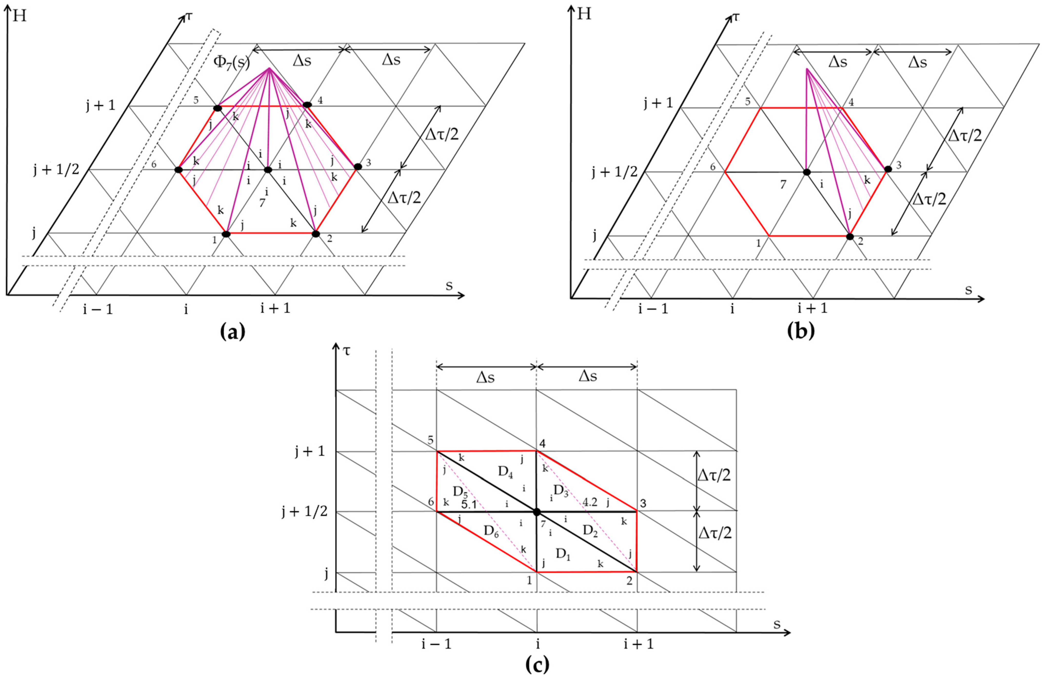
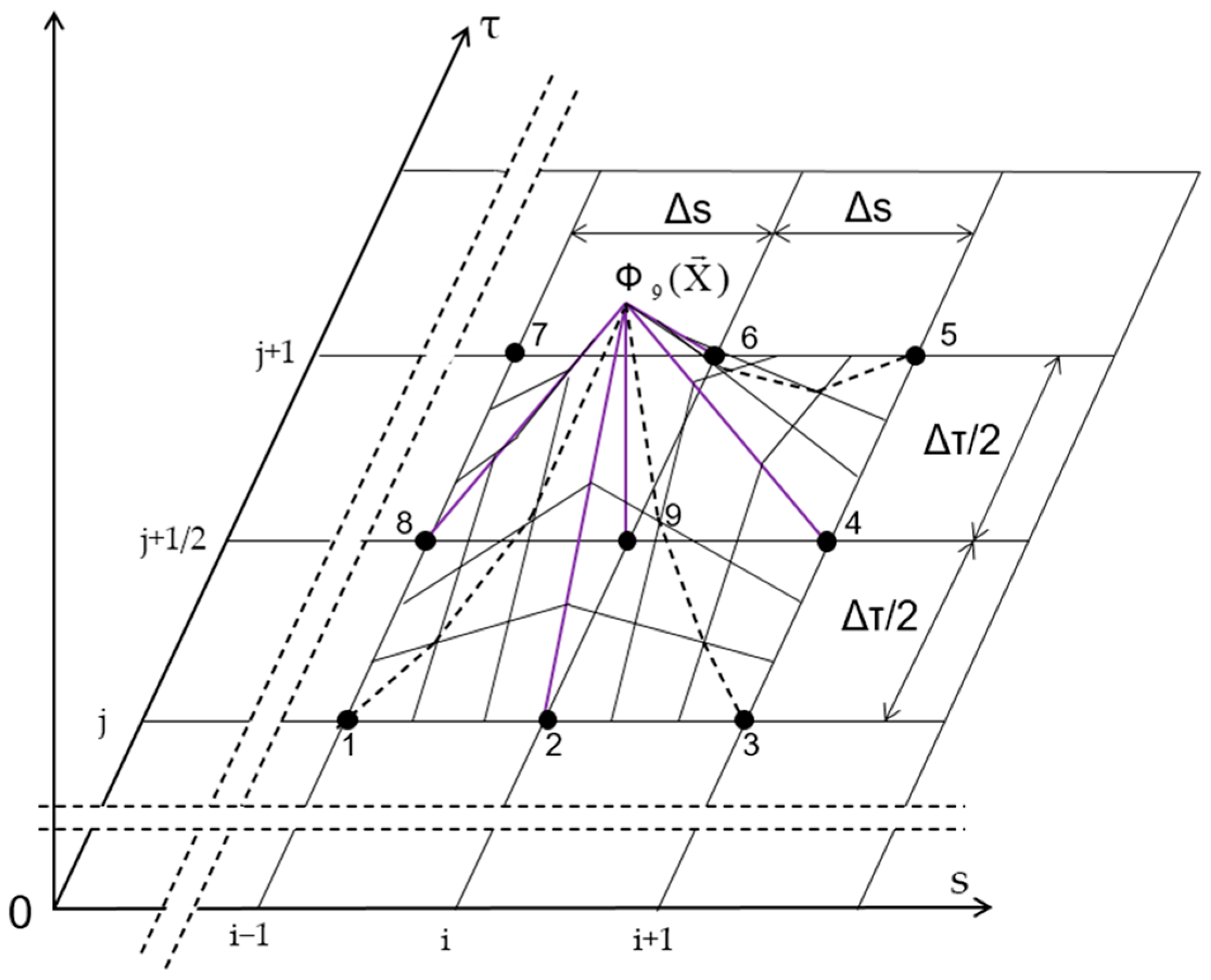
2.3.2. The Proposed Fuzzy Triangular Finite Element Solution

We have taken six α-cuts for the ratio ${\nu }_{{\alpha }_i}=({\displaystyle \frac{K}{S}}{)}_{{\alpha }_i},\left(i=\mathrm{1,2}, \dots ,6\right),$ and the above systems (cases a and b) are solved for every ${\nu }_{{\alpha }_i},(i=\mathrm{1,2}, \dots ,6)$. It is easy to solve once the non-dimensional form of the above system has solutions for every α-cut and every system as follows.

From Equation (3) we have

$$\tau ={\displaystyle \frac{K{h}_{0}t}{2S{L}^2}},\mathrm{or} {\tau }_{{\alpha }_i}=({\displaystyle \frac{K}{S}}{)}_{{\alpha }_i}{\displaystyle \frac{h_0}{2L^2}}{t}_{{\alpha }_i}$$

(15)

where α_i means the α-cut in line i. For simplification, we put the ratio $({\displaystyle \frac{K}{S}}{)}_{{\alpha }_i}={\nu }_{{\alpha }_i}$, and the above relation becomes

$${\tau }_{{\alpha }_i}={\nu }_{{\alpha }_i}{\displaystyle \frac{h_0}{2L^2}}{t}_{{\alpha }_i}$$

For α = 1, we have from Figure 3 ${\alpha }_6\left|\alpha =1\right.$, and the α-cut ${\alpha }_6$ = 1 is taken as a basis for the ratio $({\displaystyle \frac{K}{S}}{)}_{{\alpha }_i}={\nu }_{{\alpha }_i}$ that means ${\tau }_{{\alpha }_6}={\nu }_{{\alpha }_6}{\displaystyle \frac{h_0}{2L^2}}{t}_{{\alpha }_6}$.

For two different α-cuts ${\alpha }_i,{ \alpha }_j$ we take

$${\displaystyle \frac{{\tau }_{{\alpha }_i}}{{\tau }_{{\alpha }_j}}}={\displaystyle \frac{{\nu }_{{\alpha }_i}}{{\nu }_{{\alpha }_j}}}{\displaystyle \frac{t_{{\alpha }_i}}{t_{{\alpha }_j}}}\Rightarrow {\tau }_{{\alpha }_i}={\tau }_{{\alpha }_j}{\displaystyle \frac{{\nu }_{{\alpha }_i}}{{\nu }_{{\alpha }_j}}}{\displaystyle \frac{t_{{\alpha }_i}}{t_{{\alpha }_j}}}$$

(16)

and for the same real time $t_{{\alpha }_i}=t_{{\alpha }_j}$ we have

$${\tau }_{{\alpha }_i}={\tau }_{{\alpha }_j}{\displaystyle \frac{{\nu }_{{\alpha }_i}}{{\nu }_{{\alpha }_j}}}.$$

(17)

Therefore, for the solutions of case a, as well as for the case b, the solutions of the crisp non dimensional system (8) and the linearized Equation (11) are sufficient in order to have the solutions of the two cases. For every real time $t_{{\alpha }_i}=t_{{\alpha }_j}$, the non-dimensional time ${\tau }_{{\alpha }_i}$ of every α-cut is given by Equation (17). The α-cut ${\alpha }_6\left|\alpha =1\right.$ is taken as a basis in Equation (17) and this equation becomes

$${\tau }_{{\alpha }_i}={\nu }_{{\alpha }_i}\left({\displaystyle \frac{{\tau }_{{\alpha }_6=1}}{{\nu }_{{\alpha }_6=1}}}\right),$$

(18)

That is, the non-dimensional time for each α-cut is the product of the ratio $({\displaystyle \frac{K}{S}}{)}_{{\alpha }_i}={\nu }_{{\alpha }_i}$ and the ratio $\left({\displaystyle \frac{{\tau }_{{\alpha }_6=1}}{{\nu }_{{\alpha }_6=1}}}\right).$

2.3.3. Outflow Volumes

The outflow volume for dimensional variables is equal to

$$\Omega \left(t_i\right)={\int }_0^{L}Sh(x,t_i)dx (m^3/m),$$

or in non-dimensional variables

$$V\left({\tau }_i\right)={\displaystyle \frac{\Omega \left(t_i\right)}{S{h}_{0}L}}={\int }_0^{1}H(s,{\tau }_i)ds.$$

In the case of fuzzy numbers, we have

$$\left[V\right({\tau }_i){]}_{{\alpha }_i}=[{\int }_0^{1}H(s,{\tau }_i)ds{]}_{{\alpha }_i}.$$

It is now easy to find fuzzy estimators of outflow volume for each time τ_i.

2.4. Proposed Method for Solving the Crisp and Fuzzy Cases of Non-Dimensional Variables

For the convenience of the reader, the following pseudocode (Algorithem 1) is presented in the following explanatory form:

Algorithem 1 A pseudocode solving process
Step 1:	τ = 0 The interval [s0, sN] is divided into N equal parts: $\Delta s={\displaystyle \frac{(s_N-s_0)}{N}},s_r=s_0+(r-1)\Delta s,r=\mathrm{1,2},\dots ,N+1,s_0=0,s_N=1$
Step 2:	τ = τ+Δτ, $\lambda ={\displaystyle \frac{\Delta \tau }{\Delta s^2}}$
Step 3:	Initial values H(sr,0)  sr, r = 1,2,…N + 1
Step 4:	Boundary values H(0,τ) = h0, ${\displaystyle \frac{dH(s_{N+1},\tau )}{ds}}=0\to {\displaystyle \frac{H(s_{N+2},\tau )-H(s_N,\tau )}{2\Delta s}}=0\to H(s_{N+2},\tau )=H(s_N,\tau )$
Step 5:	Find coefficients $\overline{A_i,B_i,C_i,D_i}$
Step 6:	Solve the tridiagonal system [36,37]
Step 7:	Put HNEW into HINITIAL
Step 8:	Compute outflow volume V(HNEW)
Step 9:	Print τ, V(τ), HΝΕW values
Step 10:	If $\tau \le {\tau }_{\max }$ go to 2
	end

3. Results

In order to test the efficiency of the proposed fuzzy triangular finite element solution with other methods, the Boussinesq fuzzy analytical solution and the fuzzy orthogonal finite element method [35] are used. A soil sample was used with the following parameters: a hydraulic conductivity K with mean value of 3 cm/h and standard deviation and an effective porosity S with mean value of 0.21 and standard deviation. In both cases, the magnitude of the measurements is equal to n = 40 and the two parameters follow a normal distribution. This soil is classified as coarse sand according to the classification of [47].

3.1. Boussinesq Analytical Solution

Boussinesq (1904) [2] obtained an exact analytical solution assuming an inverse incomplete beta function as the initial condition for the ground water table. His solution was obtained under simplifying assumptions:

(a)

Neglecting the effect of capillary rise above the water table;

(b)

Accepting the Dupuit–Forcheimer approximation, i.e., the hydraulic head is independent of depth and therefore the streamlines are assumed to be approximately parallel to the bed;

(c)

His solution is valid when t is large, that is, when the water table at x = L is below the aquifer depth h₀ (See Figure 1).

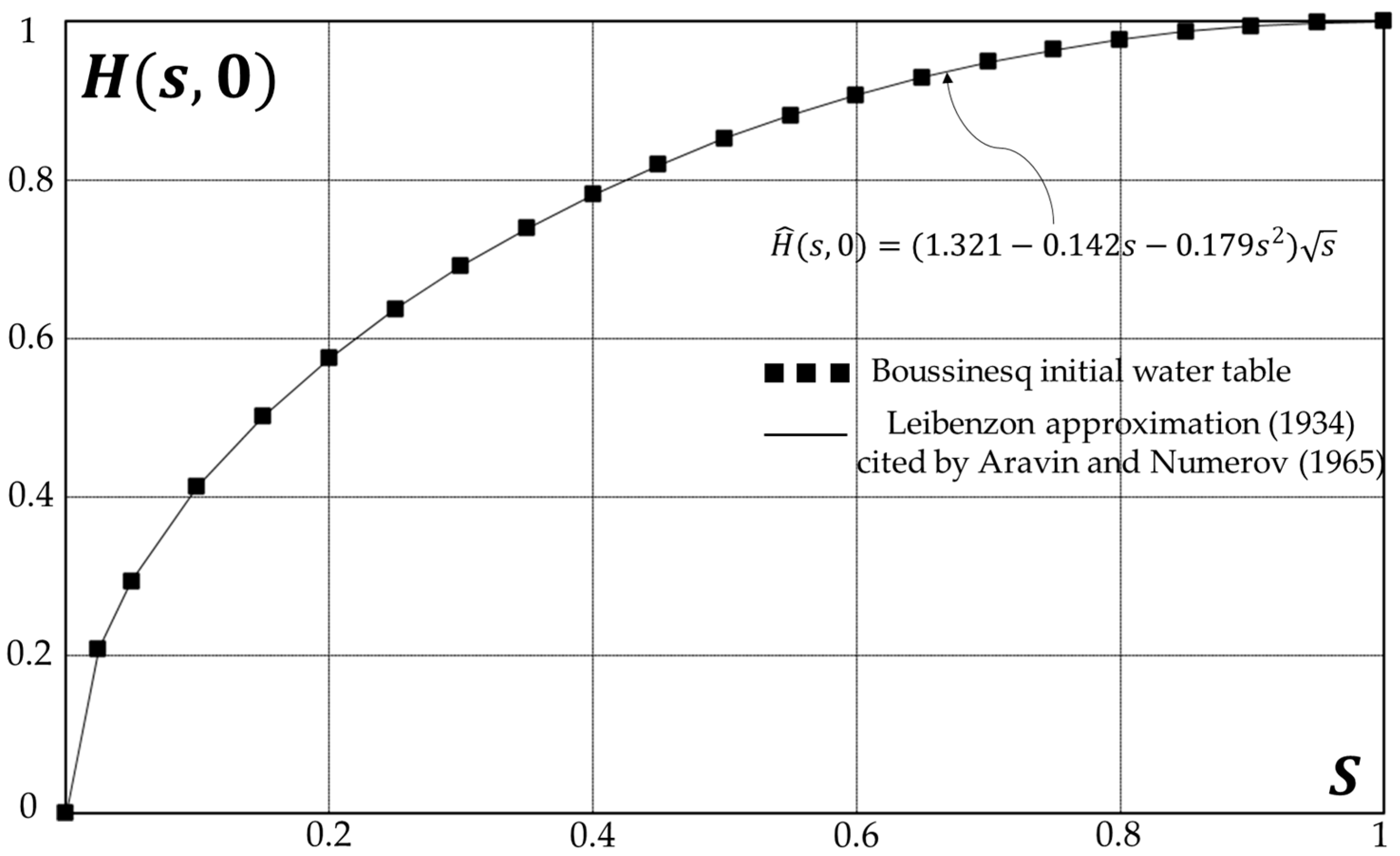
3.2. Initial Water Table

The final value for each time is given by Boussinesq in the following form:

$$H\left(s,\tau \right)={\displaystyle \frac{H\left(s,0\right)}{1+1.115\ast \tau }}, \tau ={\displaystyle \frac{K{h}_{0}t}{S{L}^2}}$$

where H(s, 0) is the initial condition for the ground water table. Leibenzon (1934), cited by Aravin and Numerov (1965) [48], gives for H(s, 0) the following approximated expression:

$$H(s,0)=(1.321-0.142s-0.179s^2)\sqrt{s}$$

Note: in the present research, the value of ${\tau }_1={\displaystyle \frac{K{h}_{0}t}{2S{L}^2}}={\displaystyle \frac{\tau }{2}}\Rightarrow \tau =2{\tau }_1$.

3.3. Storativity and Discharge

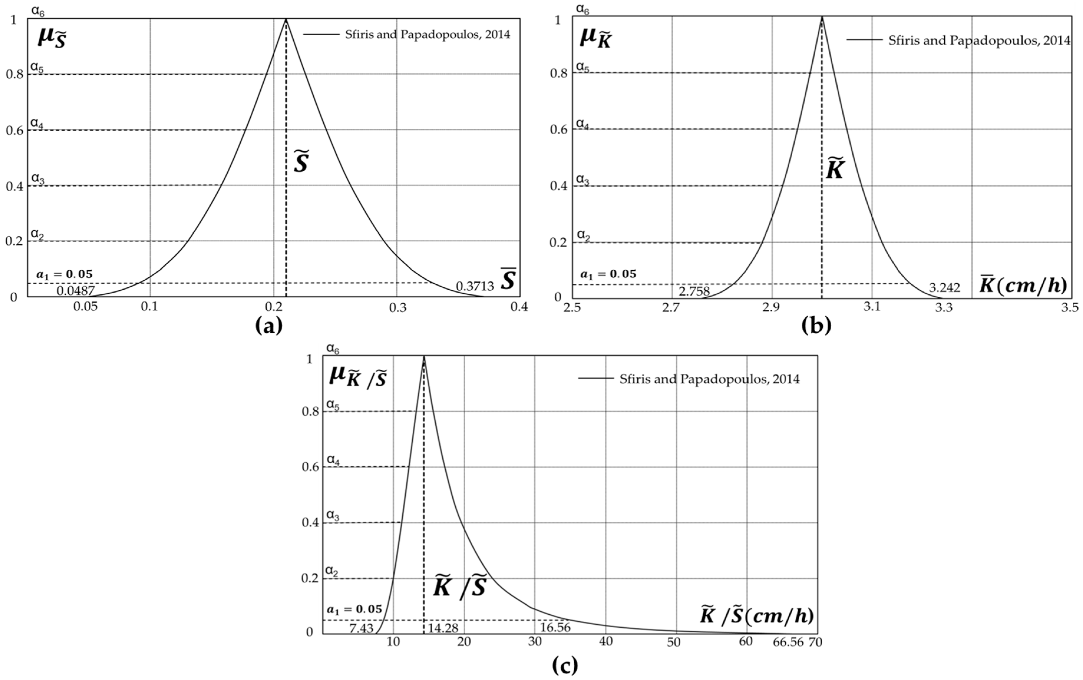
3.3.1. Dimensional Storativity

$${\Omega }_{init}=\left(SB{h}_0\right){\int }_0^{1}H\left(s,0\right)ds,$$

where S = effective porosity and B = aquifer breath.

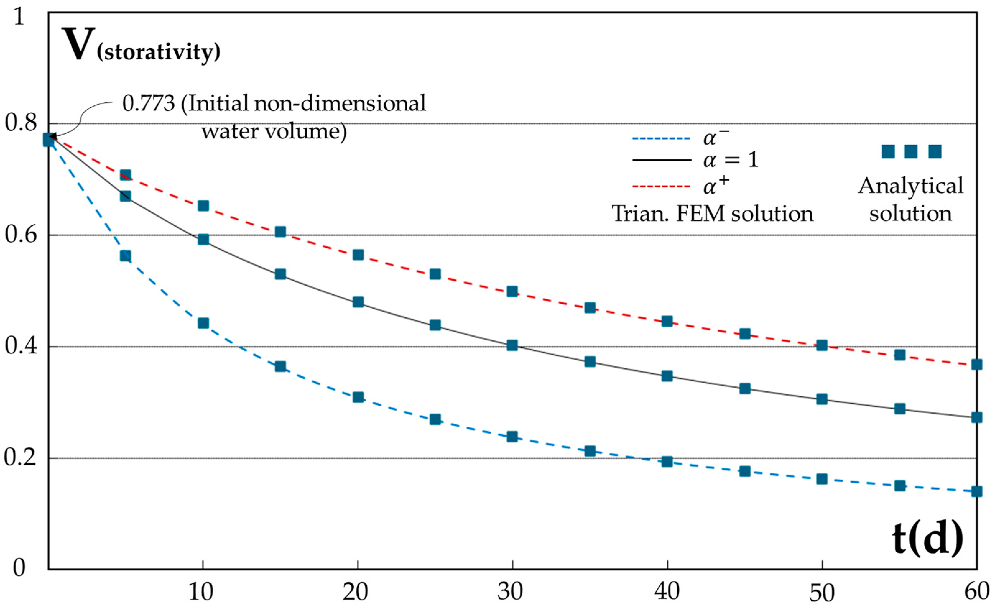
3.3.2. Non-Dimensional Storativity

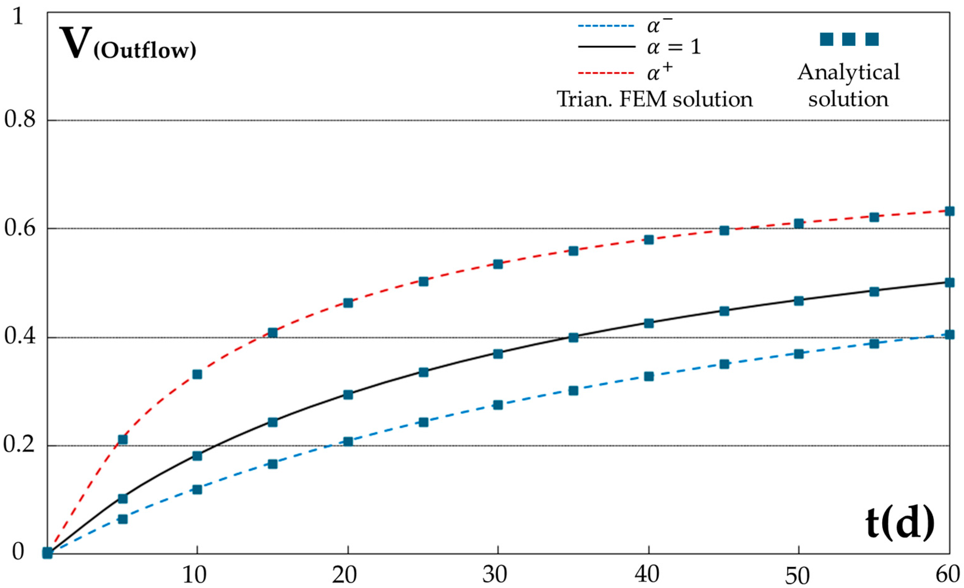
$$V_{\mathrm{init}}={\displaystyle \frac{{\mathsf{\Omega }}_{init}}{SL{h}_0}}={\int }_0^{1}H(s,0)ds={\displaystyle \frac{2}{3C}}=0.773096, C=0.86236$$

Applying now the Leibenzon approximated expression, we have

$$V_{init}^{\prime }={\int }_0^{1}H(s,0)ds={\int }_0^1(1.321-0.142s-0.179s^2)\sqrt{s}=0.772724$$

The reduced error between Vinit and V′init is equal to

$$\epsilon ={\displaystyle \frac{\left|V_{init}-V_{init}^{\prime }\right|}{V_{init}}}=4.8·10^{-4}$$

that is, the Leibenzon approximation is very reliable. Figure 4 presents the Boussinesq initial curve and Leibenzon approximation.

3.3.3. Discharge

The discharge Q per unit width is equal to ${\displaystyle \frac{dV}{d\tau }}={\displaystyle \frac{0.86236}{(1+1.115\tau {)}^2}}$.

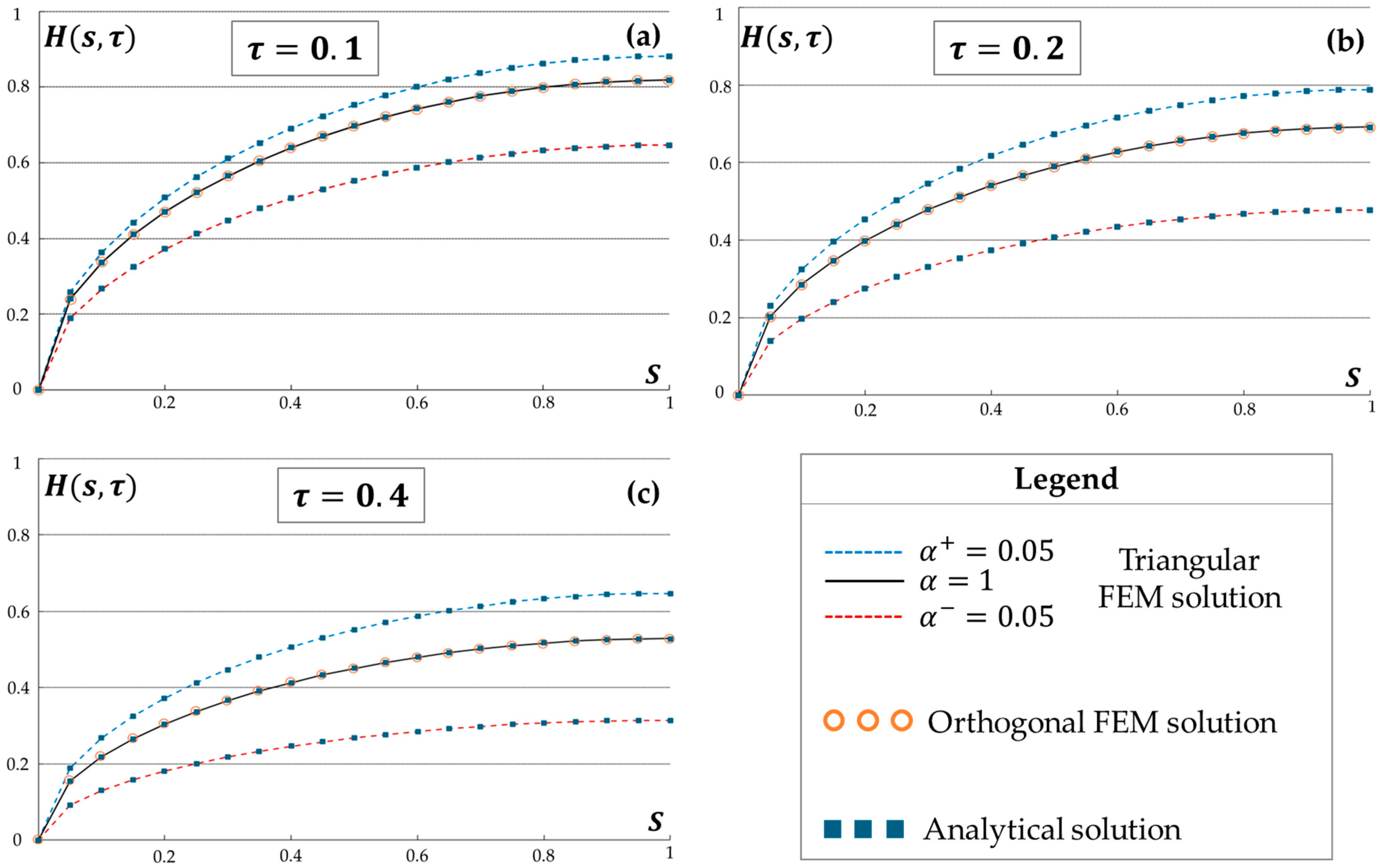
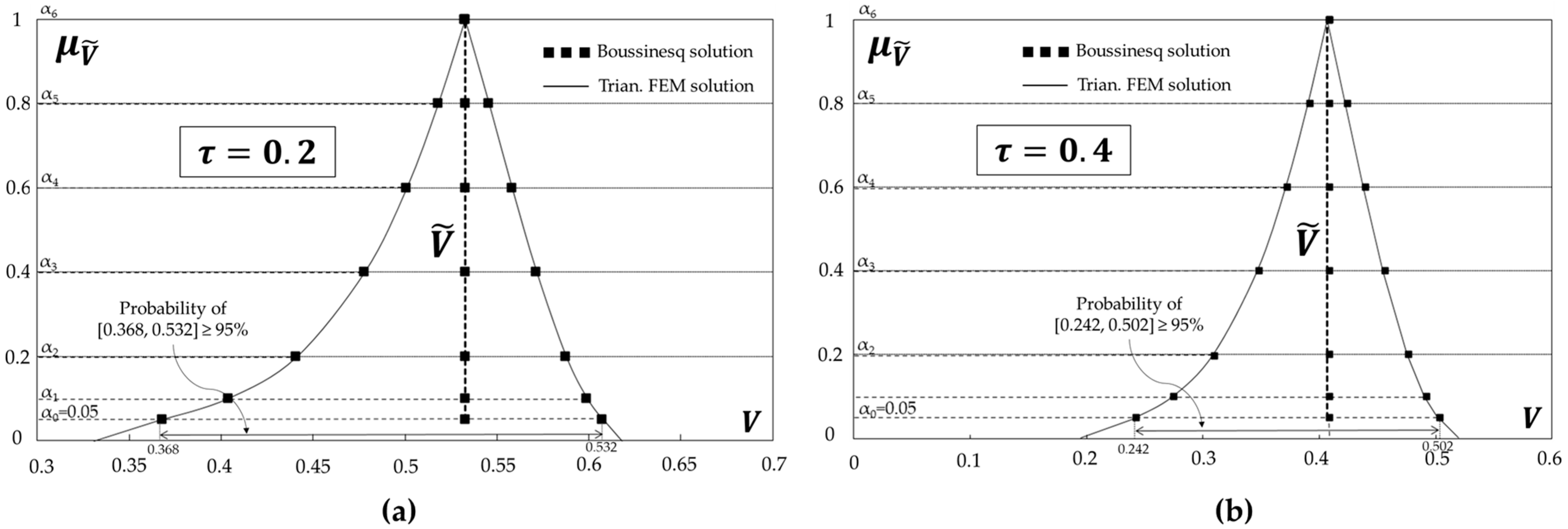
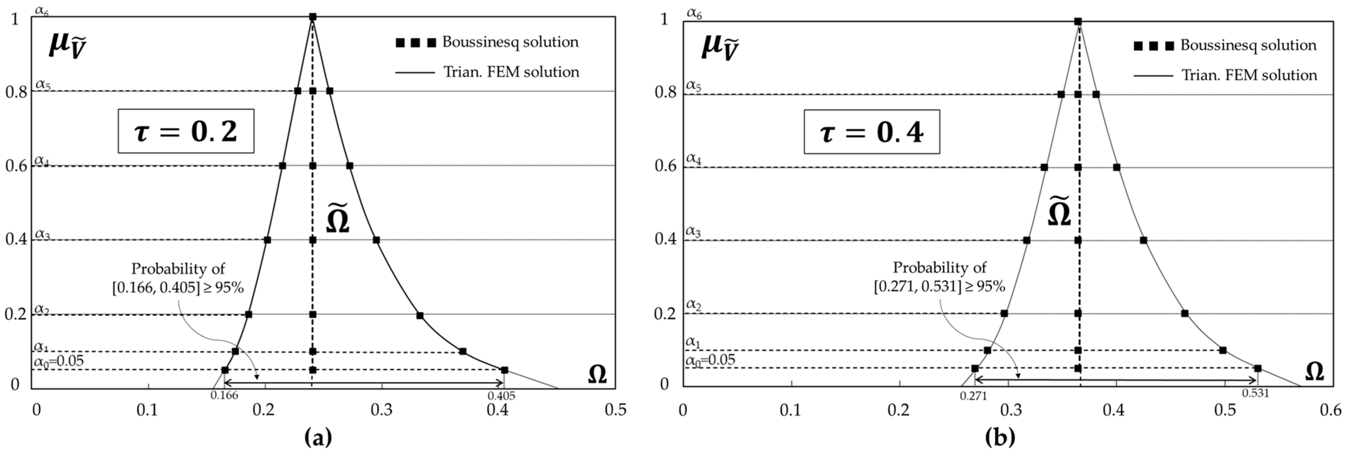
3.4. Fuzzy Triangular Finite Element Method Application and Comparison

For comparison needs, a short presentation of the orthogonal fuzzy FEM is presented below with the corresponding graphical representation (Figure 5).

The linearized FEM model is [35]

$$\begin{array}{c}{A}_i{X}_{i-1,j+1}+B_i{X}_{i,j+1}+C_i{X}_{i+1,j+1}=D_i\\ A_i=-\lambda H_{i-1,j}+{\displaystyle \frac{1}{6}},B_i=2\lambda H_{i,j}+{\displaystyle \frac{2}{3}},C_i=-\lambda H_{i+1,j}+{\displaystyle \frac{1}{6}},D_i={\displaystyle \frac{1}{6}}(H_{i+1,j}+4H_{i,j}+H_{i-1,j})\\ X_{i-1,j+1}\equiv H_{i-1,j+1},X_{i,j+1}\equiv H_{i,j+1},X_{i+1,j+1}\equiv H_{i+1,j+1}\end{array}$$

According to the above theory, which is presented in Section 2, a code program was constructed for triangular FEM, as described above for the crisp case. For the fuzzy case, it has used the method of different time spaces described above. The initial Boussinesq curve was calculated using the Leibenzon approximation

$$H(s,0)=(1.321-0.142s-0.179s^2)\sqrt{s}$$

with Δs = 0.05. Figure 6 illustrates the falling of the water level for three different times (τ = 0.1, τ = 0.2, and τ = 0.4) using the FEM.

Table 1. Values of H(s,τ) for τ = 0.2.

	ORTH Fuzzy FEM			TRIAN Fuzzy FEM			Boussinesq
a/a	${\mathit{\tau }}_{{\mathit{\alpha }}^{-}}$ 0.48959	${\mathit{\tau }}_{{\mathit{\alpha }}^{-}}={\mathit{\tau }}_{{\mathit{\alpha }}^{+}}$ 0.20000	${\mathit{\tau }}_{{\mathit{\alpha }}^{+}}$ 0.12002	${\mathit{\tau }}_{{\mathit{\alpha }}^{-}}$ 0.48959	${\mathit{\tau }}_{{\mathit{\alpha }}^{-}}={\mathit{\tau }}_{{\mathit{\alpha }}^{+}}$ 0.20000	${\mathit{\tau }}_{{\mathit{\alpha }}^{+}}$ 0.12002	${\mathit{\tau }}_{{\mathit{\alpha }}^{-}}$ 0.48959	${\mathit{\tau }}_{{\mathit{\alpha }}^{-}}={\mathit{\tau }}_{{\mathit{\alpha }}^{+}}$ 0.20000	${\mathit{\tau }}_{{\mathit{\alpha }}^{+}}$ 0.12002
0.00	0.00000	0.00000	0.00000	0.00000	0.00000	0.00000	0.00000	0.00000	0.00000
0.05	0.13991	0.20232	0.23077	0.13991	0.20240	0.23077	0.14041	0.20311	0.23169
0.10	0.19702	0.28490	0.32496	0.19702	0.28501	0.32496	0.19729	0.28541	0.32555
0.15	0.23987	0.34686	0.39564	0.23987	0.34700	0.39564	0.23990	0.34703	0.39586
0.20	0.27500	0.39766	0.45358	0.27500	0.39781	0.45357	0.27482	0.39758	0.45349
0.25	0.30493	0.44094	0.50294	0.30493	0.44111	0.50294	0.30460	0.44068	0.50263
0.30	0.33095	0.47856	0.54585	0.33095	0.47875	0.54585	0.33052	0.47815	0.54541
0.35	0.35382	0.51164	0.58358	0.35382	0.51184	0.58358	0.35335	0.51113	0.58308
0.40	0.37405	0.54089	0.61695	0.37405	0.54110	0.61695	0.37358	0.54039	0.61645
0.45	0.39197	0.56681	0.64651	0.39197	0.56703	0.64651	0.39152	0.56639	0.64606
0.50	0.40783	0.58974	0.67266	0.40784	0.58997	0.67266	0.40742	0.58935	0.67230
0.55	0.42182	0.60996	0.69572	0.42182	0.61020	0.69572	0.42146	0.60968	0.69547
0.60	0.43406	0.62766	0.71591	0.43406	0.62790	0.71591	0.43376	0.62746	0.71576
0.65	0.44467	0.64300	0.73341	0.44467	0.64325	0.73341	0.44442	0.64288	0.73336
0.70	0.45373	0.65610	0.74835	0.45373	0.65635	0.74835	0.45353	0.65609	0.74838
0.75	0.46130	0.66705	0.76083	0.46130	0.66731	0.76083	0.46113	0.66708	0.76093
0.80	0.46744	0.67593	0.77096	0.46744	0.67619	0.77096	0.46729	0.67600	0.77109
0.85	0.47219	0.68279	0.77878	0.47219	0.68305	0.77878	0.47203	0.68285	0.77892
0.90	0.47556	0.68767	0.78435	0.47556	0.68793	0.78435	0.47539	0.68769	0.78446
0.95	0.47759	0.69060	0.78769	0.47759	0.69087	0.78769	0.47740	0.69059	0.78777
1.00	0.47772	0.69087	0.78804	0.47772	0.69113	0.78804	0.47806	0.69156	0.78887

presents the values of the water table H(s, τ) for τ = 0.2 and

Table 2. Values of H(s, τ) for τ = 0.4.

	ORTH Fuzzy FEM			TRIAN Fuzzy FEM			Boussinesq
a/a	${\mathit{\tau }}_{{\mathit{\alpha }}^{-}}$ 0.97917	${\mathit{\tau }}_{{\mathit{\alpha }}^{-}}={\mathit{\tau }}_{{\mathit{\alpha }}^{+}}$ 0.40000	${\mathit{\tau }}_{{\mathit{\alpha }}^{+}}$ 0.24004	${\mathit{\tau }}_{{\mathit{\alpha }}^{-}}$ 0.97917	${\mathit{\tau }}_{{\mathit{\alpha }}^{-}}={\mathit{\tau }}_{{\mathit{\alpha }}^{+}}$ 0.40000	${\mathit{\tau }}_{{\mathit{\alpha }}^{+}}$ 0.24004	${\mathit{\tau }}_{{\mathit{\alpha }}^{-}}$ 0.97917	${\mathit{\tau }}_{{\mathit{\alpha }}^{-}}={\mathit{\tau }}_{{\mathit{\alpha }}^{+}}$ 0.40000	${\mathit{\tau }}_{{\mathit{\alpha }}^{+}}$ 0.24004
0.00	0.00000	0.00000	0.00000	0.00000	0.00000	0.00000	0.00000	0.00000	0.00000
0.05	0.09194	0.15466	0.19058	0.09194	0.15466	0.19058	0.09225	0.15523	0.19130
0.10	0.12947	0.21779	0.26836	0.12947	0.21779	0.26836	0.12963	0.21813	0.26880
0.15	0.15763	0.26515	0.32673	0.15763	0.26515	0.32673	0.15763	0.26522	0.32685
0.20	0.18071	0.30398	0.37457	0.18071	0.30399	0.37457	0.18057	0.30386	0.37444
0.25	0.20038	0.33707	0.41534	0.20038	0.33707	0.41534	0.20014	0.33680	0.41501
0.30	0.21748	0.36583	0.45078	0.21748	0.36583	0.45078	0.21717	0.36543	0.45033
0.35	0.23251	0.39112	0.48194	0.23251	0.39112	0.48194	0.23217	0.39064	0.48143
0.40	0.24581	0.41348	0.50949	0.24581	0.41348	0.50949	0.24546	0.41300	0.50898
0.45	0.25759	0.43329	0.53390	0.25759	0.43329	0.53390	0.25725	0.43288	0.53343
0.50	0.26801	0.45082	0.55551	0.26801	0.45082	0.55551	0.26770	0.45042	0.55510
0.55	0.27720	0.46628	0.57455	0.27720	0.46628	0.57455	0.27692	0.46596	0.57423
0.60	0.28524	0.47981	0.59122	0.28525	0.47981	0.59122	0.28501	0.47955	0.59099
0.65	0.29222	0.49154	0.60567	0.29222	0.49154	0.60567	0.29201	0.49133	0.60551
0.70	0.29817	0.50155	0.61801	0.29817	0.50155	0.61801	0.29799	0.50143	0.61792
0.75	0.30315	0.50992	0.62833	0.30315	0.50992	0.62833	0.30299	0.50983	0.62828
0.80	0.30719	0.51671	0.63669	0.30719	0.51671	0.63669	0.30704	0.51665	0.63667
0.85	0.31031	0.52196	0.64315	0.31031	0.52196	0.64315	0.31015	0.52188	0.64313
0.90	0.31253	0.52569	0.64775	0.31253	0.52569	0.64775	0.31236	0.52558	0.64771
0.95	0.31386	0.52793	0.65051	0.31386	0.52793	0.65051	0.31368	0.52780	0.65044
1.00	0.31392	0.52809	0.65075	0.31392	0.52809	0.65075	0.31411	0.52854	0.65134

presents the values of the water table H(s, τ) for τ = 0.4.

Both tables have been divided in three groups: ORT fuzzy FEM, TRIAN fuzzy FEM, and the Boussinesq analytical method. In front of each group, there are three numbers. For instance, in the first group in Table 1, there are the three numbers 0.48959, 0.2, and 0.12002. The middle number corresponds to non-dimensional time τ = 0.2 and according to Equation (3) it is

$${\tau }_{0.2}=0.2={\displaystyle \frac{K{h}_{0}t}{2S{L}^2}}=({\displaystyle \frac{K}{S}}{)}_{\alpha =1}{\displaystyle \frac{h_0}{2L^2}}{t}_{\tau =0.2}=14.285({\displaystyle \frac{h_0}{2L^2}})t_{\tau =0.2}\Rightarrow t_{\tau =0.2}={\displaystyle \frac{0.2}{14.285}}{\displaystyle \frac{2L^2}{S}}$$

In Figure 3c, in level α = 0.05, there are two values:

$$({\displaystyle \frac{K}{S}}{)}_{{\alpha }_{0.05}^{-}}=7.42, ({\displaystyle \frac{K}{S}}{)}_{\alpha {+}_{0.05}^{-}}=66.56$$

We consider now the same dimensional time $t_{\tau =0.2}$ for both α-secs (${\alpha }_{0.5}^{-},{\alpha }_{0.5}^{+}$) and we have

$${\tau }_{1new}==7.42{\displaystyle \frac{h_0}{2L^2}}{t}_{\tau =0.2}\to {\tau }_{new}={\displaystyle \frac{7.42}{14.285}}0.2=0.12002$$

$${\tau }_{2new}==66.56{\displaystyle \frac{h_0}{2L^2}}{t}_{\tau =0.2}\to {\tau }_{new}={\displaystyle \frac{66.56}{14.285}}0.2=0.48949$$

These new values for non-dimensional times

$${\tau }_{1new}=0.12002 \mathrm{a}\mathrm{n}\mathrm{d} {\tau }_{2new}=0.48949$$

correspond to levels ${\alpha }_{0.05}^{-},{ \alpha }_{0.05}^{+}$ of the dimensional time $t_{\tau =0.2}$.

According to the above tables, it is obvious that the orthogonal fuzzy FEM is in close agreement with the triangular fuzzy FEM. In order to make a comparison between the triangular fuzzy FEM method and Boussinesq analytical solution, the mean reduced square error is introduced as follows:

$$e={\displaystyle \frac{1}{N}}\sum _{j=1}^N{\left({\displaystyle \frac{H_{TridFEM,j}^{{\alpha }_i}-H_{Bous,j}^{{\alpha }_i}}{H_{Bous,j}^{{\alpha }_i}}}\right)}^2$$

Table 3. Mean reduced square error.

TRIAN Fuzzy FEM vs. Boussinesq
	${\mathit{\alpha }}^{-}$	$\mathit{\alpha }=1$	${\mathit{\alpha }}^{+}$
${\tau }_1$	0.0000011292	0.0000011775	0.0000011763
${\tau }_2$	0.0000012431	0.0000012289	0.0000011372
${\tau }_4$	0.0000013667	0.0000011672	0.0000011166

presents the mean reduced square error between the TRID fuzzy FEM and Boussinesq solution. In all cases, the error is small and the mean error of all is equal to 1.19 × 10⁻⁶.

Figure 7 and Figure 8 illustrate the water storativity versus real time and the water outflow versus real time, correspondingly. The fine line corresponds to triangular fuzzy FEM solution and the black orthogonal points correspond to the Boussinesq analytical solution. In both Figures, there is a good agreement between the two solutions.

Figure 9 illustrates the fuzzy estimator of water storativity V for τ = 0.2 and τ = 0.4. The fine line corresponds to the triangular fuzzy FEM solution and the black orthogonal points correspond to the Boussinesq analytical solution. According to these figures, the probability of interval [0.368, 0.532] is greater than 95‰ for τ = 0.2 and the probability of interval [0.242, 0.502] is greater than 95‰ for τ = 0.4. Finally, Figure 10 illustrates the water outflow volume Ω, in which the fine line corresponds to the triangular fuzzy FEM solution, the black orthogonal points correspond to the Boussinesq analytical solution, and the two lines on either side represent the α-cuts (α⁻, α⁺). The probability of interval [0.166, 0.405] is greater than 95‰ for τ = 0.2 and the probability of interval [0.271, 0.531] is greater than 95‰ for τ = 0.4.

4. Discussion

The study of drought flow presents unique challenges due to its dependence on complex hydrological and hydraulic processes. Unlike steady-state or fully saturated flow conditions, drought flow is characterized by low water availability, an increased influence of capillary forces, and strong interactions between soil properties and subsurface flow pathways. These conditions necessitate numerical methods that can handle irregular geometries, nonlinear boundary conditions, and uncertainty in parameter estimation.

Traditional numerical techniques, such as FDM and FVM, have proven useful in solving various fluid dynamics problems. However, these methods struggle when applied to domains with complex geometries and heterogeneous boundary conditions, which are common in drought-affected regions. Moreover, drought flow is influenced by uncertain parameters characterized also by great spatial variability, such as K and S. This issue necessitates advanced fuzzy numerical schemes such as the fuzzy FEM, which, against other fuzzy numerical methods [49,50], provides a more flexible approach by discretizing the study region into small, interconnected elements, especially with the use of triangular elements, as proposed in the current work. This approach enhances the classical FEM framework by incorporating fuzzy logic principles, enabling the model to handle the uncertainties inherent in drought flow predictions. In addition, this allows FEM to approximate governing equations efficiently, even in irregular domains, and capture accurately the properties’ variations and provide more realistic simulations of subsurface flow. Especially, based on the findings of this work, the use of triangular elements allows for better convergence properties in computational models, reducing the errors associated with numerical discretization and improving stability in the low-flow conditions characteristic of drought events. Additionally, traditional FEM approaches often require precise input parameters, which may be difficult to obtain in drought-prone regions. By incorporating fuzzy sets, the proposed triangular fuzzy FEM mitigates the impact of parameter estimation errors and allows for a more comprehensive sensitivity analysis.

Beyond handling uncertainties in hydraulic parameters, in this work, the integration of probability theory through fuzzy estimators introduces a new dimension of reliability in hydrological modeling. Based on our results, the fuzzy estimators for water storativity (V) and water outflow (Ω) using the possibility theory provide strong probabilities (95%) with a small risk margin (5%) for their values, providing a more realistic physical condition of the investigated problem.

Overall, the benefit gained through the application of this methodology is substantial, especially for engineers involved in the design and construction of hydraulic projects. Specifically, by quantifying uncertainties more effectively and providing probability-based confidence intervals, the method allows engineers to achieve a reliable evaluation of study quality and project performance, with an overall reliability exceeding 95%. This capability is crucial in practice, where uncertainty in soil and hydraulic parameters can significantly affect project outcomes. Traditional deterministic methods often underestimate such uncertainties, leading to potential risks in both the design and construction phases. In contrast, the integration of fuzzy logic within the finite element framework enables better risk management, more informed decision-making, and, ultimately, greater project success. From an academic perspective, this research advances the state of knowledge by offering a robust and flexible methodology that can handle irregular geometries, highly variable hydraulic properties, and uncertainty quantification—areas where traditional methods face limitations.

Despite its advantages, the triangular fuzzy FEM has certain limitations that must be acknowledged. One key challenge is the increased computational cost associated with the incorporation of fuzzy logic into the finite element framework. The additional complexity introduced by fuzzy membership functions and possibility theory increases the number of calculations required, potentially leading to longer simulation times compared to traditional FEM approaches. This issue may be particularly limiting for large-scale hydrological models or real-time decision-making applications. Furthermore, while the proposed triangular fuzzy FEM improves the representation of uncertainties in hydraulic properties, it does not eliminate the need for calibration and validation using observed data. The effectiveness of the method relies on thorough validation against experimental or field measurements, which may not always be available for drought-prone regions. In addition, the integration of probability-based fuzzy estimations into FEM is still an evolving field, requiring further theoretical advancements and practical testing to refine its applicability.

Future research should focus on refining fuzzy membership functions, optimizing computational efficiency, and validating model outcomes with field observations to further improve its applicability to similar physical problems. Moreover, future studies should explore the extension of probability-based fuzzy estimations to other hydrological parameters, such as soil moisture retention and infiltration rates, to provide a more holistic understanding of subsurface flow processes. Finally, expanding the application of the proposed FEM scheme to other hydrological processes, such as the hydraulic communication of surface and aquifer systems and ecohydrological modeling, could provide a more comprehensive understanding of water dynamics in drought-prone regions.

5. Conclusions

This research makes a significant contribution to the advancement of uncertainty modeling in hydrological systems by developing a novel triangular fuzzy finite element method (FEM) framework for drought flow analysis. The integration of triangular fuzzy logic with FEM, grounded in the generalized Hukuhara derivative (gH-derivative) theory for partial differential equations, represents a substantial theoretical innovation that extends existing fuzzy calculus to practical hydraulic modeling. Compared to traditional numerical approaches, it provides a more robust and flexible framework capable of handling irregular geometries, highly variable hydraulic properties, and the inherent uncertainties in hydrological processes.

The implementation of Galerkin’s method within this fuzzy FEM framework offers a rigorous and efficient solution approach for nonlinear and uncertainty-laden hydrological problems. Our comparative analysis shows that the triangular fuzzy FEM achieves excellent agreement with both the orthogonal fuzzy FEM and the analytical solution of the Boussinesq equation, demonstrating a mean reduced square error of $1.19·{10}^{-6}$ across all cases. This confirms the method’s high reliability and predictive accuracy.

Importantly, this work advances the academic field by providing a probabilistically sound methodology for integrating fuzzy estimators of hydraulic parameters directly into finite element formulations. By enabling uncertainty quantification through possibility theory, fuzzy confidence intervals, and conjecture theory, the proposed approach empowers engineers and researchers to make more informed decisions under conditions of limited or imprecise data.

In summary, the triangular fuzzy FEM developed in this study not only strengthens the theoretical foundations of fuzzy hydrological modeling but also enhances practical applications in areas such as irrigation management, groundwater conservation, and drought mitigation planning. It stands as a valuable addition to the scientific community’s toolkit for addressing complex water resource challenges under uncertainty.

References

1. Hall, F.R. Base-Flow Recessions—A Review. Water Resour. Res. 1968, 4, 973–983. [Google Scholar] [CrossRef]
2. Boussinesq, J. Recherches Theoriques Sur l’ecoulement Des Nappes d’eau Infiltrees Dans Le Sol et Sur Le Debit Des Sources. J. Math. Pures Appl. 1904, 10, 5–78. [Google Scholar]
3. Brutsaert, W.; Nieber, J.L. Regionalized Drought Flow Hydrographs from a Mature Glaciated Plateau. Water Resour. Res. 1977, 13, 637–643. [Google Scholar] [CrossRef]
4. Troch, P.A.; De Troch, F.P.; Brutsaert, W. Effective Water Table Depth to Describe Initial Conditions Prior to Storm Rainfall in Humid Regions. Water Resour. Res. 1993, 29, 427–434. [Google Scholar] [CrossRef]
5. Szilagyi, J.; Parlange, M.B.; Albertson, J.D. Recession Flow Analysis for Aquifer Parameter Determination. Water Resour. Res. 1998, 34, 1851–1857. [Google Scholar] [CrossRef]
6. Troch, P.A.; van Loon, A.H.; Hilberts, A.G.J. Analytical Solution of the Linearized Hillslope-storage Boussinesq Equation for Exponential Hillslope Width Functions. Water Resour. Res. 2004, 40, W08601. [Google Scholar] [CrossRef]
7. Troch, P.A.; Berne, A.; Bogaart, P.; Harman, C.; Hilberts, A.G.J.; Lyon, S.W.; Paniconi, C.; Pauwels, V.R.N.; Rupp, D.E.; Selker, J.S.; et al. The Importance of Hydraulic Groundwater Theory in Catchment Hydrology: The Legacy of Wilfried Brutsaert and Jean-Yves Parlange. Water Resour. Res. 2013, 49, 5099–5116. [Google Scholar] [CrossRef]
8. Bartlett, M.S.; Porporato, A. A Class of Exact Solutions of the Boussinesq Equation for Horizontal and Sloping Aquifers. Water Resour. Res. 2018, 54, 767–778. [Google Scholar] [CrossRef]
9. Akylas, E.; Gravanis, E. Approximate Solutions of the Boussinesq Equation for Horizontal Unconfined Aquifers During Pure Drainage Phase. Water 2024, 16, 2984. [Google Scholar] [CrossRef]
10. Richtmyer, R.D.; Morton, K.W. Difference Methods for Initial-Value Problems; John Wiley & Sons: New York, NY, USA; London, UK; Sidney, Australia, 1967. [Google Scholar]
11. Patankar, S.V. Numerical Heat Transfer and Fluid Flow; CRC Press: Boca Raton, FL, USA, 2018; ISBN 9781315275130. [Google Scholar]
12. Argyris, J.H. Energy Theorems and Structural Analysis. Aircr. Eng. Aerosp. Technol. 1954, 26, 383–394. [Google Scholar] [CrossRef]
13. Zienkiewicz, O.C.; Cheung, Y.K. Finite Element Method in Structural & Continuum Mechanics Hardcover, 1st ed.; McGraw Hill: London, UK, 1967. [Google Scholar]
14. Oden, J.T. Finite Elements of Nonlinear Continua; Dover Publications: New York, NY, USA, 1972. [Google Scholar]
15. Oden, J.T. Historical Comments on Finite Elements. In A History of Scientific Computing; ACM: New York, NY, USA, 1990; pp. 152–166. [Google Scholar]
16. Tzimopoulos, C. Solution de l’équation de Boussinesq par une méthode des éléments finis. J. Hydrol. 1976, 30, 1–18. [Google Scholar] [CrossRef]
17. Galerkin, B.G. Rods and Plates: Series in Some Questions of Elastic Equilibrium of Rods and Plates; National Technical Information Service: Springfield, VA, USA, 1968. [Google Scholar]
18. Frangakis, C.N.; Tzimopoulos, C. Unsteady Groundwater Flow on Sloping Bedrock. Water Resour. Res. 1979, 15, 176–180. [Google Scholar] [CrossRef]
19. Tzimopoulos, C.; Tolikas, P. ICID Bulletin (International Commission on Irrigation and Drainage); ICID: New Delhi, India, 1980; pp. 40–44. [Google Scholar]
20. Tber, M.H.; El Alaoui Talibi, M. A Finite Element Method for Hydraulic Conductivity Identification in a Seawater Intrusion Problem. Comput. Geosci. 2007, 33, 860–874. [Google Scholar] [CrossRef]
21. Mohammadnejad, T.; Khoei, A.R. An Extended Finite Element Method for Hydraulic Fracture Propagation in Deformable Porous Media with the Cohesive Crack Model. Finite Elem. Anal. Des. 2013, 73, 77–95. [Google Scholar] [CrossRef]
22. Yang, D.; Zhou, Y.; Xia, X.; Gu, S.; Xiong, Q.; Chen, W. Extended Finite Element Modeling Nonlinear Hydro-Mechanical Process in Saturated Porous Media Containing Crossing Fractures. Comput. Geotech. 2019, 111, 209–221. [Google Scholar] [CrossRef]
23. Aslan, T.A.; Temel, B. Finite Element Analysis of the Seepage Problem in the Dam Body and Foundation Based on the Galerkin’s Approach. Eur. Mech. Sci. 2022, 6, 143–151. [Google Scholar] [CrossRef]
24. Puri, M.L.; Ralescu, D.A. Differentials of Fuzzy Functions. J. Math. Anal. Appl. 1983, 91, 552–558. [Google Scholar] [CrossRef]
25. Hukuhara, M. Integration Des Applications Measurables Dont La Valeur Est Un Compact Convexe. Funkc. Ekvacioj 1967, 10, 205–233. [Google Scholar]
26. Kaleva, O. Fuzzy Differential Equations. Fuzzy Sets Syst. 1987, 24, 301–307. [Google Scholar] [CrossRef]
27. Seikkala, S. On the Fuzzy Initial Value Problem. Fuzzy Sets Syst. 1987, 24, 319–330. [Google Scholar] [CrossRef]
28. Vorobiev, D.; Seikkala, S. Towards the Theory of Fuzzy Differential Equations. Fuzzy Sets Syst. 2002, 125, 231–237. [Google Scholar] [CrossRef]
29. Nieto, J.J.; Rodríguez-López, R. Bounded Solutions for Fuzzy Differential and Integral Equations. Chaos Solitons Fractals 2006, 27, 1376–1386. [Google Scholar] [CrossRef]
30. Diamond, P. Brief Note on the Variation of Constants Formula for Fuzzy Differential Equations. Fuzzy Sets Syst. 2002, 129, 65–71. [Google Scholar] [CrossRef]
31. Bede, B.; Gal, S.G. Generalizations of the Differentiability of Fuzzy-Number-Valued Functions with Applications to Fuzzy Differential Equations. Fuzzy Sets Syst. 2005, 151, 581–599. [Google Scholar] [CrossRef]
32. Bede, B. A Note on “Two-Point Boundary Value Problems Associated with Non-Linear Fuzzy Differential Equations”. Fuzzy Sets Syst. 2006, 157, 986–989. [Google Scholar] [CrossRef]
33. Stefanini, L. A Generalization of Hukuhara Difference and Division for Interval and Fuzzy Arithmetic. Fuzzy Sets Syst. 2010, 161, 1564–1584. [Google Scholar] [CrossRef]
34. Allahviranloo, T.; Gouyandeh, Z.; Armand, A.; Hasanoglu, A. On Fuzzy Solutions for Heat Equation Based on Generalized Hukuhara Differentiability. Fuzzy Sets Syst. 2015, 265, 1–23. [Google Scholar] [CrossRef]
35. Tzimopoulos, C.; Papadopoulos, K.; Samarinas, N.; Papadopoulos, B.; Evangelides, C. Fuzzy Finite Elements Solution Describing Recession Flow in Unconfined Aquifers. Hydrology 2024, 11, 47. [Google Scholar] [CrossRef]
36. Thomas, L.H. Elliptic Problems in Linear Difference Equations over a Network; Watson Scientific Computing Laboratory at Columbia University: New York, NY, USA, 1949. [Google Scholar]
37. Samarinas, N.; Tzimopoulos, C.; Evangelides, C. An Efficient Method to Solve the Fuzzy Crank–Nicolson Scheme with Application to the Groundwater Flow Problem. J. Hydroinformatics 2022, 24, 590–609. [Google Scholar] [CrossRef]
38. Zadeh, L.A. Fuzzy Sets. Inf. Control 1965, 8, 338–353. [Google Scholar] [CrossRef]
39. Negoita, C.V.; Ralescu, D.A. REPRESENTATION THEOREMS FOR FUZZY CONCEPTS. Kybernetes 1975, 4, 169–174. [Google Scholar] [CrossRef]
40. Goetshel, R.; Voxman, W. Elementary Fuzzy Calculus. Fuzzy Sets Syst. 1986, 18, 31–43. [Google Scholar] [CrossRef]
41. Bede, B.; Stefanini, L. Generalized Differentiability of Fuzzy-Valued Functions. Fuzzy Sets Syst. 2013, 230, 119–141. [Google Scholar] [CrossRef]
42. Khastan, A.; Nieto, J.J. A Boundary Value Problem for Second Order Fuzzy Differential Equations. Nonlinear Anal. Theory Methods Appl. 2010, 72, 3583–3593. [Google Scholar] [CrossRef]
43. Dubois, D.; Foulloy, L.; Mauris, G.; Prade, H. Probability-Possibility Transformations, Triangular Fuzzy Sets, and Probabilistic Inequalities. Reliab. Comput. 2004, 10, 273–297. [Google Scholar] [CrossRef]
44. Mylonas, N. Applications in Fuzzy Statistic and Approximate Reasoning. Ph.D. Thesis, Dimokritos University of Thrace, Komotini, Greece, 2022. [Google Scholar]
45. Sfiris, D.S.; Papadopoulos, B.K. Non-Asymptotic Fuzzy Estimators Based on Confidence Intervals. Inf. Sci. 2014, 279, 446–459. [Google Scholar] [CrossRef]
46. Tzimopoulos, C.; Papadopoulos, K.; Evangelides, C.; Papadopoulos, B. Fuzzy Solution to the Unconfined Aquifer Problem. Water 2018, 11, 54. [Google Scholar] [CrossRef]
47. Domenico, P.A.; Schwartz, F.W. Physical and Chemical Hydrogeology, 2nd ed.; John Wiley and Sons, Inc.: Hoboken, NJ, USA, 1990. [Google Scholar]
48. Aravin, V.I.; Numerov, S.N. Theory of Fluid Flow in Deformable Porous Media; Israel Program for Scientific Translation: Jerusalem, Israel, 1948. [Google Scholar]
49. Samarinas, N.; Tzimopoulos, C.; Evangelides, C. Fuzzy Numerical Solution to Horizontal Infiltration. Int. J. Circuits Syst. Signal Process. 2018, 12, 326–332. [Google Scholar]
50. Samarinas, N.; Tzimopoulos, C.; Evangelides, C. Fuzzy Numerical Solution to the Unconfined Aquifer Problem under the Boussinesq Equation. Water Supply 2021, 21, 3210–3224. [Google Scholar] [CrossRef]
Figure 1. Sketch of the definition of the investigated problem.
Hydrology 12 00128 g001
Figure 2. Finite element model: (a) global basis function, (b) local basis function, and (c) normal grid.
Hydrology 12 00128 g002
Figure 3. Fuzzy estimators of (a) S, (b) K, and (c) the ratio K/S, where αi (i = 1,2,…,6) are α-cuts [45].
Hydrology 12 00128 g003
Figure 4. Boussinesq initial curve and Leibenzon approximation [2,48].
Hydrology 12 00128 g004
Figure 5. Orthogonal FEM model.
Hydrology 12 00128 g005
Figure 6. Ground water levels H vs. non-dimensional time τ. Comparison of the fuzzy triangular FEM method with the Boussinesq analytical method and with the fuzzy orthogonal FEM method for (a) τ = 0.1, (b) τ = 0.2, and (c) τ = 0.4.
Hydrology 12 00128 g006
Figure 7. Water storativity versus real time t(d).
Hydrology 12 00128 g007
Figure 8. Water outflow versus real time t(d).
Hydrology 12 00128 g008
Figure 9. Fuzzy estimator of water storativity for (a) τ = 0.2 and (b) τ = 0.4.
Hydrology 12 00128 g009
Figure 10. Fuzzy estimator of water outflow for (a) τ = 0.2 and (b) τ = 0.4.
Hydrology 12 00128 g010