Abstract
This study evaluated ten drought indices focusing on their ability to monitor drought events in Marathwada, a semi-arid region of India. High-resolution gridded monthly total precipitation data for 75 years (1950–2024) from the European Centre for Medium-Range Weather Forecasts (ECMWF) were used to evaluate the drought indices. These indices were computed across six timescales: 1, 3, 4, 6, 9, and 12 months. A Generalized Autoregressive Conditional Heteroscedastic (GARCH) model was employed to detect temporal volatility in precipitation, followed by a second-order geospatial autocorrelation eigenfunction eigendecomposition using Global Moran’s Index statistics to geolocate both aggregated and non-aggregated precipitation locations. The performance of drought indices was assessed using non-parametric Spearman’s correlation to identify the strength, direction, and similarity of regional-specific drought events. The temporal lag interdependence between meteorological and agricultural droughts was assessed using a non-parametric Spearman’s cross correlation function (SCCF). The findings revealed that the GARCH model with a skewed Student’s t distribution effectively captured conditional temporal volatility and asymptotic behavior in the precipitation series. The model’s sensitivity enabled the incorporation of temporal fluctuations related to droughts and extreme meteorological events. The Bhalme and Mooley Drought Index (BMDI-6) and Z-Score Index (ZSI-6) were the most applicable indices for drought monitoring. Spearman’s cross-correlation analysis revealed that meteorological droughts influenced agricultural droughts with a time lag of up to 4 months.
1. Introduction
Drought is an extended duration of precipitation deficit compared to the long-term climatological mean, resulting in negative moisture anomalies, leading to soil moisture depletion, inadequate water supply, reduced soil moisture, and substantial agricultural damage []. The Indian Meteorological Department (IMD) defines drought as a rainfall deficiency exceeding 25% of its long-term mean, typically over a period of at least 30 years. Hydrologists have broadly classified droughts into four types: meteorological, agricultural, hydrological, and socio-economic [,]. In recent decades, drought frequency, intensity, and spatial extent have increased globally due to climate variability and increasing water demands []. Droughts pose significant risks to water security, agriculture, and livelihoods [,]. Their effects, however, can be minimized through timely monitoring, precision forecasting, and implementation of early warning systems [].
The Indian subcontinent is highly prone to droughts due to its reliance on monsoon-driven agriculture and increasing climatic variability. Severe droughts have already impacted India’s water resources and crop productivity [], and future climate projections suggest an increased drought risk []. In recent years, the Marathwada region of Maharashtra has experienced irregular monsoon patterns, leading to recurrent droughts and heatwaves, resulting in crop failures, thereby threatening the livelihoods of farmers and the broader socio-economic stability of the region [].
Drought events are monitored using drought indices based on statistical calculations involving precipitation to estimate the onset, intensity, duration, and termination periods of droughts []. While various drought indices have been formulated to evaluate and monitor drought spells, their accuracy and reliability can vary across different climatic regimes, particularly due to differences in the statistical distribution of precipitation []. For instance, semi-arid regions often exhibit highly skewed and non-Gaussian precipitation patterns, which may violate the assumptions of certain drought indices [,,]. Thus, evaluating the regional performance and sensitivity of drought indices is crucial for enhancing early warning systems and mitigating extreme hydrometeorological risks in drought-vulnerable zones such as Marathwada.
Several studies have analyzed drought conditions using both advanced time series models and nonparametric methods. For instance, Uddin et al. [] employed an sGARCH model to detect precipitation volatility in Bangladesh and reported its limitations in modeling rainfall variability due to persistent high volatility. However, Bouznad et al. [] employed ARIMA (Autoregressive Integrated Moving Average) models using precipitation, temperature, and evapotranspiration data to forecast seasonal drought conditions in Algerian highlands and found that ARIMA provided robust forecasts based on its lower error metrics. In contrast, Ghost et al. [] implemented a hybrid ARIMA-GARCH model for monitoring crop yield and forecasting in the semi-arid region of India, highlighting its efficiency in detecting temporal volatility and seasonal fluctuations compared to the sGARCH model. Furthermore, both parametric and non-parametric methods have been used widely for drought assessment. For instance, Tidjeman et al. [] compared parametric and non-parametric methods for monitoring hydrological droughts and reported that the most optimal choice of method depends on the selected distribution and its goodness-of-fit measures. Similarly, recent studies have evaluated the performance of drought indices using both parametric and non-parametric correlation and reported that non-parametric tests are more efficient in both detecting non-linear drought patterns and assessing the similarity of drought events [,]. Additionally, the non-parametric Spearman’s cross-correlation function has been employed to quantify the time lag between meteorological and agricultural droughts [,].
Past studies have widely focused on the Standardized Precipitation Index (SPI) to analyze drought regimes across various hydroclimatic variability, including the USA, Europe, Africa, and Asia [,,]. Similarly, recent studies have evaluated the performance of drought indices at regional and river basin levels [,,]. However, the previous studies focused on a limited number of indices, including the SPI [], ZSI (Z-Score Index; []), and CZI (China Z-Index; []) at different time steps in India. No authors have tested the Bhalme and Mooley Drought Index (BMDI) index for the semi-arid region of India, which was developed specifically for monsoon-based drought monitoring and surveillance []. Moreover, these indices were compared using the linear Pearson correlation methodology, which assumes linear relationships [,]. However, this method does not fully capture the inherent non-linear complexities (zero autocorrelation and geospatial timeseries volatility) []. These indices often exhibit skewed and asymmetric behavior, especially in semi-arid regions, where climate variability introduces conditional volatility, conditional outliers, and unconditional variance, thereby violating the assumptions of the parametric test. These non-Gaussian distributions can reduce the accuracy of drought pattern detection []. A few researchers have identified non-zero autocorrelation patterns within precipitation datasets [,] but have not quantified the temporal volatility. This unquantified temporal volatility with non-Gaussian zero autocorrelation can generate geographical chaos [] in precipitation data, leading to non-robust and biased drought indices output [].
The precision of drought monitoring depends on accurately capturing the temporal variability in precipitation over time []. Most drought indices are based on unconditional variance, assuming that the mean and standard deviation remain constant over a long-term climatological baseline []. However, in monsoon-dominated regions like India, temporal volatility violates the assumption of stationarity inherent in these models, as precipitation variance shifts annually across seasons []. In the semi-arid region of Marathwada, precipitation patterns are characterized by short, intense monsoon spells, followed by extended dry periods, which could lead to heterogeneity in rainfall distribution and variance. These heterogeneous patterns can introduce volatility and non-stationarity, violating the assumptions of homogeneous variance in SPI []. Furthermore, SPI is highly sensitive to the length of the reference period under non-stationary conditions []. To address these temporal shifts, the Generalized Autoregressive Conditional Heteroscedastic (GARCH) model [] offers a robust alternative by precisely estimating conditional variance, where past precipitation shocks influence present variability []. This approach stabilizes variance and mitigates volatility effects, enabling drought indices to accurately reflect both short-term fluctuations and long-term extremes. Consequently, GARCH can enhance the detection of drought onset, duration, and the impact of a changing climate, which is particularly relevant for the Marathwada region.
Unlike unconditional models that assume static variance, GARCH-based conditional variance adds flexibility by the ability to model time-varying precipitation volatility, enabling drought indices to respond to both gradual shifts and abrupt anomalies in precipitation []. This is particularly important for improving drought early warning systems, where indices often fail to detect the intensification or sudden onset of events []. Neglecting such volatility and non-stationarity in precipitation data can result in overestimation or underestimation of drought severity, leading to biased drought estimation [], which has been a limitation in previous studies. Hence, there is a need for modelling approaches that account for temporal volatility and non-stationarity, particularly under finite-sampled non-asymptotic conditions in precipitation data.
India’s southwest monsoon (June to September) is quintessential in shaping the country’s drought dynamics []. Despite its importance, limited research has focused on evaluating drought indices during this four-month monsoon period, which is essential for seasonal drought monitoring and agricultural planning. While SPI is globally recognized, it may not always capture short-term droughts, particularly on a monthly and quarterly basis, in semi-arid monsoon-dominated regions like India [,]. Despite its importance, the non-Gaussian nature of precipitation and the impacts of heteroscedasticity have rarely been examined in a spatiotemporal context []. These issues may violate the assumptions of Tobler’s First Law of Geography, which assumes stronger relationships among nearby precipitation grid points [], undermining the robustness of drought assessments. A comparative analysis of multiple drought indices would ensure rigorous validation and could identify context-specific alternatives, thereby improving the precision of drought detection and agricultural risk assessment. To overcome these research limitations, this study aims to
- (1)
- examine zero autocorrelation coefficients using the second-order semi-parametric eigenfunction eigendecomposition algorithm;
- (2)
- implement the GARCH model to analyze the temporal volatility, persistence, and extreme events of drought conditions;
- (3)
- compare ten drought indices to assess the severity and duration of historical drought events across multiple timescales;
- (4)
- analyze the temporal lagged association between meteorological and agricultural droughts.
2. Study Area
This study was conducted for the Marathwada region of central India, which comprises nine districts with a total area of approximately 64,590 square kilometers (Figure 1). Marathwada is situated in the central part of Maharashtra state, spanning from 17°35′ to 20°41′ N latitude and 74°40′ to 78°16′ E longitude. The region is topographically characterized by flat-topped basaltic hills formed by the Deccan Traps. It lies in the leeward slope of the Western Ghats (Sahyadri ranges), resulting in reduced monsoonal rainfall and recurrent droughts. The windward side of the Ghats receives higher rainfall due to orographic lifting, whereas Marathwada, located on the drier leeward side, experiences semi-arid conditions, classified as BSh (hot semi-arid) under the Köppen climate classification []. These climatic contrasts contribute to pronounced regional variations in drought intensity and frequency.

Figure 1.
Study area.
The region’s elevation ranges from approximately 221 meters to 1528 meters above sea level (Figure 1). According to the Indian Meteorological Department (IMD), Marathwada experiences three major seasons: summer (March–May), southwest monsoon (June–September), and winter (October–February). The average rainfall ranges from 750 to 800 mm during the monsoon season, which is significantly lower than the national average of approximately 1200 mm. During the summer season, temperatures fluctuate between 36 °C and 45 °C, with May being the hottest month. Winter temperatures typically range from 10 to 15 °C, with December being the coldest month. The detailed descriptive statistics are given in Table 1.

Table 1.
Statistical Summary of Total Precipitation.
In recent years, the Marathwada region has been increasingly affected by extreme weather events, including recurring droughts, prolonged heat waves, and hailstorms. With agriculture as the primary source of livelihood, the population remains highly vulnerable to inter-annual variability in monsoonal rainfall. Hence, even a slight shift in rainfall timing or amount of rainfall can trigger major crop failures and socioeconomic consequences, highlighting Marathwada’s critical status as a climate-sensitive hotspot for drought impact assessment and resilience planning.
3. Materials and Methods
3.1. Data Collection
A monthly gridded dataset of total precipitation (TP), with a spatial resolution of 0.1° latitude by 0.1° longitude, was obtained from the ERA5-Land reanalysis dataset developed by the European Centre for Medium-Range Weather Forecasts (ECMWF; []). The dataset (version 1) was accessed on 10 March 2024, through the Copernicus Climate Data Store (CDS; DOI: https://doi.org/10.24381/cds.e2161bac). This dataset included TP values for 696 land-based grid cells, covering all nine districts of the Marathwada region from 1950 to 2024.
The ERA5-Land-based TP data were re-gridded from their original 0.1° × 0.1° resolution to 0.5° × 0.5° longitude using a conservative, area-weighted cartographic method [] to match the spatial resolution of the Indian Meteorological Department (IMD) gridded rainfall data []. ERA5-Land was validated against IMD rainfall over Marathwada using a grid-to-grid approach to ensure reliability. The agreement between the two datasets was evaluated using Pearson (r) and Spearman (ρ) correlations, along with error metrics including Kling-Gupta Efficiency (KGE), root mean square error (RMSE), standard error of mean (SEM), mean absolute error (MAE), and mean bias error (MBE).
3.2. Second Order Eigenfunction Eigendecompostion Geospatial Autocorrelation
The spatial clustering of TP was evaluated using semi-parametric eigenfunction-based second-order geospatial autocorrelation []. This method, based on Moran’s spatial filtering algorithm developed by Getis and Griffith [], identifies spatial clusters by capturing localized spatial dependencies. In this experiment, we used the eigenfunction eigendecomposition to determine aggregation/non-aggregation (‘hot/cold spots’) in TP across the study region. These clusters were identified based on the positive and negative values of Global Moran’s Index (I), computed across all grid points in the TP dataset.
We generated a latent, autocorrelated index employing the stratified TP estimator using Moran’s index (I) in ArcGIS Pro. Moran’s I was employed using the equation
where was the total number of TP grid points and W was the sum of all spatial weights. The time series TP was delineated as x, while ij was the matrix of the sampled weights. The maximum and minimum threshold values for the eigenvalue eigendecomposition, capture point, were determined employing Moran’s I, which in this experiment was provided by
where was the maximum spatial autocorrelation, and was the minimum spatial autocorrelation.
The TP grid points and their eigen-decomposed eigenvectors () were subsequently mapped in the ArcGIS Pro for each georeferenced intervention, including hot and cold spot patterns ranging from positive spatial autocorrelation to negative spatial autocorrelation for . The summary diagnostics from the model’s dependent eigen-decomposed eigenvector were equal to its associated eigenvalue, as
as V was precisely scalable to satisfy
where was the i-th eigenvalue, which indicated the magnitude of positive or negative spatial autocorrelation, was an eigen-spatial matrix, was the transpose of the matrix , was the i-th eigen-spatial eigenvector, and was the transpose of the eigen-spatial eigenvector. The n-by-1 vector x = [x1 ⋯ xn]T represented the quantitative measurements of TP values at each grid point. These locations were embedded within an n-by-n eigen-spatial weighting matrix W. The formulation for Moran’s index of eigen-time series autocorrelation was
where was the Global Moran’s Index, n was the total number of spatial grid points of TP, was a TP value at the grid point , was the mean TP value across all n grid points, was the eigen-spatial weight between two locations and derived from the eigen-spatial weight matrix, W, where and the diagonal elements are null ().
The matrix W was first extended into an asymmetrical form, and subsequently, it was further generalized into a non-symmetric matrix W* by employing
where W was the symmetrized eigen-spatial weight matrix, is the original eigen-spatial weights matrix, was the transpose of W. Moran’s I was rewritten using matrix notation:
represented a column vector containing TP values for all grid points, was the transpose of the TP vector, H was the centered TP vector value, which was computed by removing the global mean from each sampled observation. Additionally, was the sum of all weights in the matrix. In this experiment, represented an orthogonal projector satisfying the condition of H = H2, confirming its independence.
We employed Pearson’s correlation coefficient to quantify the linear relationship between TP values across georeferenced eigen-spatial grid points. The covariance between TP locations was normalized by the product of their standard deviation, as expressed below:
where was the Pearson correlation coefficient between TP at locations X and Y, was a covariance of TP, and were the standard deviations of TP, and were the means of TP, and X and Y represented the observed values of TP at those two locations. The equation of covariance between two locations was given by
where was the covariance between TP at locations X and Y, and were the means of TP at X and Y locations, was the number of TP observations. The above equations were used to capture the temporal relationships (covariance) and strength of association (Pearson’s correlation) of TP values across georeferenced hot and cold spots within predicted intervention sites. The autocorrelation model was derived using the above covariance as
where and were the largest and the smallest eigenvalues of the eigen-spatially filtered weight matrix. The eigenvalues of the spatial weight matrix were obtained through eigen-decomposition of the georeferenced TP grid point data. These eigenvalues were found to be asymptotically equivalent to Moran’s I coefficients, which were computed from the residual temporal autocorrelation and subsequently scaled by a constant factor. Eigenvectors corresponding to high positive (or negative) eigenvalues have high positive (or negative) autocorrelation []. The incorporation of these eigenvectors in Moran’s I equation resulted in
where U was the matrix containing the eigenvectors of HWH, was the diagonal matrix of eigenvalues associated with the eigenized-spatial patterns, was the transpose of the whole matrix of eigenvectors U, was the i-th eigenvalue, indicating the intensity of the non-zero eigen-spatial autocorrelation corresponding to , were the projection of TP onto the spatial pattern .
Autocovariance is defined as a function that measures the covariance of a variable with itself at different temporal lags, and is closely related to autocorrelation []. In this study, we centered the vector z = Hx, where H was an idempotent matrix. The following equation was then used to compute Global Moran’s I based on eigenvector decomposition.
where was the column vector of TP values at each grid point, was the transpose of the TP vector, was the eigen-vector of the spatial matrix W, and was the projection of TP onto the eigenized spatial pattern .
The Getis-Ord Gi algorithm [] was implemented in ArcGIS Pro to identify statistically significant geolocations of hot and cold spots in TP data using spatial clustering. This method detects high (hot spots) and low (cold spots) TP clusters at the 95% confidence level using spatial z-scores []. A 95% confidence interval (C.I.) criterion was applied to minimize Type I (e.g., geo-spatiotemporal uncommon variance) and Type II (latent geo-spatiotemporal multicollinearity) errors. We assumed that geographically aggregated hotspots (high TP values) could reveal plausible flash flood locations, while cold spots could represent regions with persistently low TP. This spatial clusterization, we assumed, would be relevant for drought monitoring in Marathwada. The study assumes that drought indices derived from statistically significant spatial clusters would provide more accurate insights into localized drought conditions in the Marathwada region.
3.3. Generalized Autoregressive Conditional Heteroscedastic (GARCH) Model
The GARCH model specified with an Autoregressive Integrated Moving Average (ARIMA) structure [] was employed to the TP time series data prior to calculating drought indices to address temporal volatility and serial autocorrelation. This ensured stationarity in the variance of TP. Non-stationary data with conditional heteroscedasticity, where variance changes over time, can inflate the standard deviation and variance. This can lead to extreme outliers and distort the accuracy of drought indices such as SPI [,]. Moreover, severe temporal volatility can distort the rank ordering of drought indices observations, which could violate the assumption of monotonicity in Spearman’s correlation []. Such violations could lead to biased (temporally heteroscedastic) correlation estimates, challenging their reliability. To address this limitation, the GARCH model was implemented to stabilize the TP time series, and the volatility-corrected TP series was then used as an input for drought indices, thereby enhancing the robustness of drought assessment.
The GARCH model generalizes Engle’s Autoregressive Conditional Heteroskedasticity (ARCH) model [] by incorporating both lagged squared error terms and lagged conditional variance over time. The ARCH model captures short-term volatility through past shocks. In contrast, the GARCH adds flexibility by incorporating both conditional heteroscedasticity and long-term volatility clustering, making it suitable for time series with persistent variance [].
In this experiment, we examined whether the variance changed over time, especially in the presence of extreme values (outliers). We aimed to determine if a thick-tailed, right-skewed distribution caused large standard deviations and high residual variance. The assumptions of the model were validated using the Augmented Dickey–Fuller (ADF) test for stationarity [], the Autoregressive Conditional Heteroscedastic Lagrange Multiplier (ARCH-LM) test for heteroscedasticity [], the Ljung–Box test for residual independence [], and the Jarque–Bera test for residual normality [].
The GARCH (1,1) model was implemented in RStudio version 2025.05.1 to capture conditional heteroscedasticity in the TP time series. The GARCH (1,1) specification was selected based on its lowest Akaike Information Criteria (AIC), Bayesian Information Criteria (BIC), and Beta (β) parameter. Additionally, the lowest Chi-square statistics, along with non-significant values of the Post-ARCH-LM and Ljung–Box tests, were also considered. The equation for modeling the conditional variance of past squared errors and past variances was defined by the following equation:
where was the conditional variance of TP at time t, was a constant baseline variance, and were the lag orders of the model, was an ARCH coefficient that measures the contribution of past TP shocks to current variance, were the squared residuals of the model at lag , was the GARCH coefficient that measured the past conditional variance of TP, and was the conditional variance of TP at lag . The equation of Student’s t error distribution is given as
where denoted the TP at time , represented an independent and identically distributed random variable, was a latent variable that followed an inverse-Gaussian distribution—, was the degree of freedom parameter that controlled the kurtosis and skewness, represented the conditional variance of TP at time t, was a baseline volatility, was an ARCH effect, > 0 was a contribution of lagged variance, was the squared TP value for the previous timestep, was the lagged conditional variance for the previous timestep.
A Student’s t distribution was employed to evaluate: (i) the effectiveness of the kurtosis coefficient to precisely model the degrees of freedom implied by heavy-tailed behavior of TP, and (ii) the efficiency of Student’s t GARCH model to evaluate the uncertainty associated with the model parameters. We hypothesized that the TP time series would exhibit heavy-tailed behavior, and both the kurtosis coefficient and Student’s t GARCH model would provide unbiased and consistent estimators of the degrees of freedom parameter.
A standardized sGARCH(1,1) and an exponential eGARCH(1,1) model were tested to evaluate symmetric and asymmetric volatility structures for robust drought indices modeling. This (1,1) structure refers to one lag of past variance and one lag of standardized residuals. Lag order was determined using the Autocorrelation Function (ACF) and Partial Autocorrelation Function (PACF). Five error distributions, including the Gaussian, Student’s t, skewed Student’s t, Generalized Error Distribution (GED), and skewed GED, were evaluated to model non-constant temporal variance associated with skewness, kurtosis, and leptokurtic or platykurtic tails. The most optimal distribution was selected based on the goodness-of-fit metrics, including the Akaike Information Criterion (AIC), Bayesian Information Criterion (BIC), and Ljung–Box test []. The Chi-square statistics with p-value of the post-ARCH-LM test were considered to validate the temporal autocorrelation and volatility modeling of TP in a GARCH model.
3.4. Drought Indices
This study incorporated ten precipitation-based drought indices to assess their severity and applicability. The criterion of precipitation-based indices was selected to maintain uniformity in input variables and to preserve the monotonicity assumption required for Spearman’s rank correlation [,]. Indices incorporating additional meteorological variables such as temperature or evapotranspiration were excluded to prevent the introduction of potential non-linear interactions that could violate this assumption.
The indices computed were the BMDI, ZSI, CZI, SPI, Percent of Normal Precipitation (PNI), Decile Index (DI), Modified CZI (mCZI), Rainfall Anomaly Index (RAI), Weighted Anomaly Standardized Precipitation (WASP), and agricultural SPI (aSPI). All the indices were computed on a monthly timestep, including the backward-moving periods of 3, 4, 6, 9, and 12 months, based on cumulative TP sums [,]. January was considered the starting month for all drought indices, reflecting the hydrologic year, to ensure consistency in long-term drought assessments on an annual basis. Additionally, a novel 4-month timescale beginning in June (rather than January) was introduced to monitor monsoon-season (June–September) droughts. This approach was implemented to capture intra-seasonal variability during the monsoon season while maintaining comparability across the hydrologic year-based indices.
3.5. Comparison of Drought Indices Based on Non-Parametric Spearman’s Rank Correlation Coefficient
The performance of continuous drought indices data was evaluated using a non-parametric Spearman’s rank correlation matrix to quantify the strength, direction, and similarity of regional-specific drought events. This approach enabled the assessment of consistency among indices for detecting drought conditions and identifying the most sensitive and reliable index for regional drought monitoring. The comparison of regional drought patterns follows the approach of previous studies that analyzed similar drought patterns [,,]. Unlike Pearson’s parametric correlation test, Spearman’s rank correlation (rho) can precisely detect linear and non-linear monotonic relationships, and does not rely on the homoscedastic, Gaussian distribution assumptions []. Hence, the correlation test is less sensitive to outliers, which are typical characteristics of drought indices time series datasets.
We generated 60 drought index time series (10 indices × 6 time steps) by performing a pairwise cross-correlation analysis of 10 drought indices for meteorological and agricultural applications at 1-, 3-, 4-, 6-, 9-, and 12-month time scales. The equation for Spearman’s rank correlation coefficient was given as
where was Spearman’s rho, was the difference between the two rank variables, and n was the total number of observations.
3.6. Drought Indices Performance Based on Severity, Time Period, and Statistical Criteria
The performance of drought indices was evaluated using the number of similar drought months across indices, drought severity classifications, and the ability to capture onset and termination periods of prolonged drought events []. These criteria were employed to assess the timely detection of droughts, sensitivity to local and regional climatic variability, the magnitude of droughts, and the onset and termination periods for the drought indices []. The severity and magnitude of drought months were computed using each index’s established threshold classification system. For instance, BMDI values ≤ −4.0 were categorized as extreme, −3.0 to −3.99 as severe, −2.0 to −2.99 as moderate, and −1.00 to −1.99 as mild drought []. Similarly, for indices such as SPI, ZSI, CZI, and mCZI, droughts were classified as extreme (<−2.0), severe (−1.5 to −1.99), and moderate (−1.0 to −1.49). The complete threshold classification system, including for the WASP index, is provided in the Supplementary Materials (Tables S1 and S2). The most prolonged drought spell was identified by computing the number of consecutive drought months and tracking the phases of drought onset and termination. Additionally, all drought indices were statistically compared against BMDI using statistical performance metrics [,] such as the coefficient of determination (R2), root mean square error (RMSE), standard error of the mean (SEM), standard error of estimate (SEE), mean absolute error (MAE), and standard deviation.
BMDI was selected as a reference index as it is a non-parametric index that directly incorporates long-term precipitation anomalies without assuming an underlying distribution []. Unlike parametric indices, such as SPI, which require fitting precipitation to a Gamma distribution that assumes homogeneous variance [], BMDI is a non-parametric index that does not require homogeneous variance, making it suitable and robust for semi-arid climates. The presence of zero-inflated TP data in the semi-arid regions can violate the Gamma distribution assumption that TP must be a continuous positive value (>0). This can deviate the empirical distribution away from the theoretical cumulative probability distribution, leading to a non-robust goodness of fit []. Such violations can cause biased estimates of the Gamma distribution’s shape (α) and scale (β) parameters [], leading to distortion of cumulative density functions (CDF), resulting in under- or over-estimation of SPI values [,]. Hence, BMDI, due to its non-parametric nature, can incorporate Poisson [], Negative Binomial [], and Log-linear distributions []. Furthermore, hierarchical Bayesian models [] provide a non-frequentist framework that can model predictive errors and outliers across space, time, and geography. The statistical performance and error metrics quantified how closely other drought indices aligned with BMDI, thereby evaluating their robustness in capturing drought timing, sensitivity, and variability [].
3.7. Non-Parametric Spearman’s Cross-Correlation Function (SCCF)
A modified cross-correlation (CCF) function, Spearman’s Cross-Correlation Function (SCCF), was employed to assess the time-lagged association between meteorological (BMDI) and agricultural (aSPI) drought conditions. Unlike Pearson’s linear CCF, which assumes linearity, Gaussian distribution, and is highly sensitive to outliers [], SCCF overcomes these limitations by detecting both linear and non-linear monotonic relationships based on a non-Gaussian distribution []. This makes SCCF particularly robust for evaluating drought indices, where time series often exhibit skewed, non-Gaussian behavior and outliers due to extreme events.
The selection of meteorological and agricultural indices was based on the performance criterion of correlation and performance-based metrics, ensuring the most statistically optimal indices were used for the SCCF analysis. BMDI was selected as the meteorological drought index because it is specifically developed for the Indian monsoon climate []. aSPI, as an agricultural drought index, incorporates effective precipitation and reflects soil moisture dynamics critical for crop-based assessments []. SCCF was applied across all time scales (1, 3, 4, 6, 9, and 12 months), and cross-correlations were computed at lags ranging from 0 to 7 months. Persistent cross-correlation across lags was analyzed to evaluate the temporal lag responses of agricultural droughts to meteorological conditions based on the statistical significance of the p-value.
4. Results and Discussion
Second-order spatial autocorrelation was employed to assess the non-random spatial clusters of TP across geospace. Subsequently, the GARCH model was employed to quantify temporal volatility in TP data. Finally, drought indices were compared using Spearman’s rank correlation, focusing on drought severity, number of drought months, and onset and termination periods.
4.1. Spatial Clustering of Total Precipitation Patterns
The spatial autocorrelation analysis of TP data revealed a Global Moran’s Index (I) of 0.93 (Table 2), suggesting a strong spatial clustering of similar TP values across surrounding geospatial grid points. High TP values indicate areas of potential flash floods, while low TP values represent plausible drought-prone zones. The high Z-score (32.93) with a statistically significant p-value demonstrated that the observed spatial clustering is unlikely due to random chance, indicating a strong positive spatial autocorrelation. These findings align with previous studies, which have reported Moran’s index exceeding 0.90 for TP clustering [,]. This structured geospatial clustering complements Tobler’s First Law of Geography [], which states that nearby clusters are more related than distant clusters, indicating the presence of strong positive spatial autocorrelation and a departure from complete spatial randomness.

Table 2.
Spatial Autocorrelation Parameters.
Additionally, the geospatial clustering of high-resolution TP at a 0.1° latitude by 0.1° longitude grid enabled the precise detection of localized hydrometeorological extremes. This resolution captured microclimatic variability across Marathwada’s windward and leeward slopes, enhancing the understanding of spatially structured drought and flood risks.
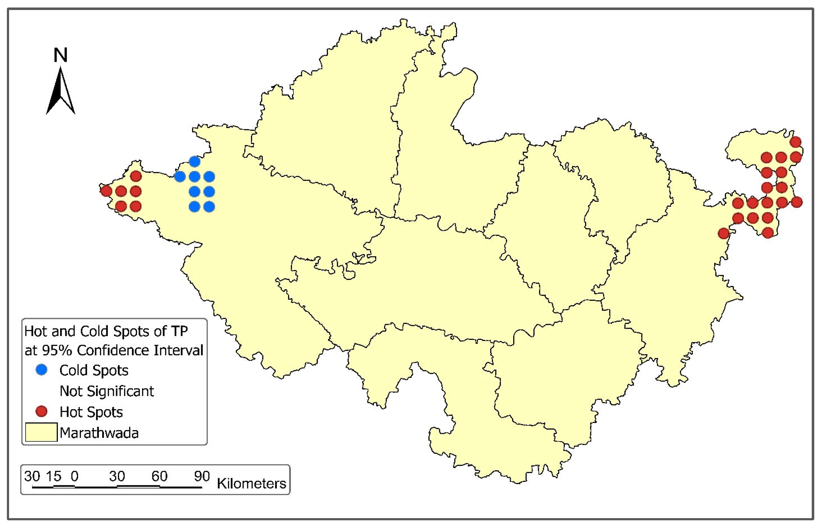
The hot and cold spots of TP at 95% C.I. reveal statistically significant spatial clustering across Marathwada (Figure 2). The cold spots were dominant in the northwestern part of the region, indicating persistent low TP zones. The cold spots were dominant in the northwest part of the region, indicating the influence of the Western Ghats’ leeward side, where persistent low TP zones occur due to the orographic process. In contrast, the eastern part of Marathwada exhibited hotspots (high TP zones), likely due to the presence of moisture-laden clouds from the Bay of Bengal. These hotspots are predominantly concentrated in agricultural zones, particularly farmlands with moderate to dense vegetation, which can enhance evapotranspiration and contribute to high TP clusters within the hydrological cycle. Conversely, the cold spots were near bare ground and settlement areas, slightly away from the farmlands, where vegetation is sparse. These spatial patterns underscore the need for region-specific water resource planning to mitigate the impacts of drought.

Figure 2.
Hot and Cold Spots of Total Precipitation.
4.2. Temporal Volatility Dynamics of Total Precipitation
The GARCH model specified with an Autoregressive Integrated Moving Average (ARIMA) structure was employed to address temporal volatility and ensure the stationarity of the TP data prior to calculating the drought index. The assumptions of the GARCH model were evaluated using the Jarque–Bera test, and the results revealed a non-Gaussian distribution of TP data. This suggests the presence of asymmetric and heavy-tailed distributions, likely driven by Marathwada’s semi-arid climate, thereby justifying the use of a flexible error distribution for the accurate modeling of conditional variance. The Augmented Dickey–Fuller (ADF) test revealed a significant statistic (−17.24; Table 3), indicating that the TP series is stationary. In contrast, the ARCH-LM test demonstrated significant temporal volatility (Chi-square = 276.02), validating the need for GARCH modeling [].

Table 3.
GARCH model parameters.
The mean equation was specified as ARIMA (5,0,1) based on the auto.arima() function in RStudio, ensuring the most optimal order (p,d,q) by minimizing AIC and BIC values. In this case, the moving average order q = 1 was chosen automatically as the best fit under this criterion. The ARIMA (5,0,1) specification indicates that TP values from the preceding five months have a significant influence on the current TP. This temporal dependence is likely due to the seasonal dynamics of the Indian monsoon, which typically occurs from June to September and sometimes extends into mid-October. These variations in TP patterns result in a substantial seasonal variation and temporal persistence, supporting the use of the ARIMA (5,1) specification [].
The sGARCH (1,1) model with a skewed Student’s t distribution revealed a relatively high baseline volatility (omega; ω = 37.01), and strong long-term volatility (beta; β = 0.99), implying a strong sensitivity to past TP shocks. In contrast, the eGARCH (1,1) model demonstrated a lower baseline volatility (ω = 6.31) and much weaker persistent volatility (β = 0.35). This suggests that past volatility has a slight contribution to model future fluctuations. However, the model is more sensitive in capturing short but intense rainfall events during the monsoon. The lower long-term volatility in the eGARCH model implied that it accommodates asymmetric responses to both positive and negative shocks more effectively than the sGARCH model. This makes the eGARCH model particularly suitable for capturing the non-linear and skewed volatility patterns of the Indian monsoon. The Sign Bias test further supported this based on the significant p-value, indicating the model’s sensitivity to asymmetric shocks. Hence, these results suggest the model’s ability to detect positive volatility shifts (plausible flash floods) and negative shifts (potential droughts), which are essential for analyzing the drought dynamics in Marathwada.
The ARIMA (5,1) specification indicated a strong fit for both sGARCH (1,1) and eGARCH (1,1) models, as revealed by low values across the AIC, BIC, Shibata, and Hannan-Quinn indices (<12). However, the overall goodness of fit was more pronounced in the eGARCH model, as demonstrated by a lower, non-significant chi-square statistic (17.07), compared to the higher, significant chi-square of the sGARCH model (70.35). The Ljung–Box test on the standardized residuals (p-value = 0.98) and squared residuals (p-value = 0.27) at lag one further confirmed the absence of serial correlation and remaining ARCH effects. This suggests a better fit and greater robustness of eGARCH in modeling non-stationary heteroscedastic TP data. The Jarque–Bera test rejected normality for both models (p-value < 0.001), indicating the presence of heavy tails and right skewness, which justifies the use of a skewed Student’s t-distribution to capture these characteristics precisely. In contrast, sGARCH exhibited significant autocorrelation in the residuals, as indicated by the post-ARCH-LM test (p-value < 0.001), suggesting that the volatility modeling was non-robust. Hence, this demonstrates that simpler models are unable to capture the heavy tails, asymmetric shocks, and time-varying volatility of TP in the monsoon-dominated region of Marathwada. Similar results were reported by Ghasempour et al. [], indicating that hybrid GARCH models are more precise than the sGARCH (1,1) for modeling monthly precipitation in the semi-arid region of Iran, particularly due to seasonal fluctuations in rainfall, such as those found in India’s monsoon patterns. Similarly, Ghosh et al. [] demonstrated that the ARIMA-eGARCH model is more efficient than the traditional models in the semi-arid region of India, highlighting their ability to capture volatility clustering under monsoon-driven rainfall variability.
The eGARCH’s ability to capture asymmetric volatility aligns with the Indian monsoon, where extreme TP and droughts may have different impacts on the volatility structure. These findings support the previous study of Modarres and Ouarda [], which demonstrated that eGARCH is more efficient than sGARCH in modeling seasonal TP volatility. This is crucial for understanding and monitoring severe seasonal drought events in hydrometeorological studies, which may exhibit potential temporal volatility in non-stationary datasets. Thus, the eGARCH model, when incorporated with the ARIMA model, can provide valuable insights into forecasting and planning the duration and severity of drought conditions for Marathwada, thereby supporting water management and agricultural decisions that rely on stable variance conditions from the ARIMA mean component.
4.3. Comparison of Drought Indices Using Spearman Correlation
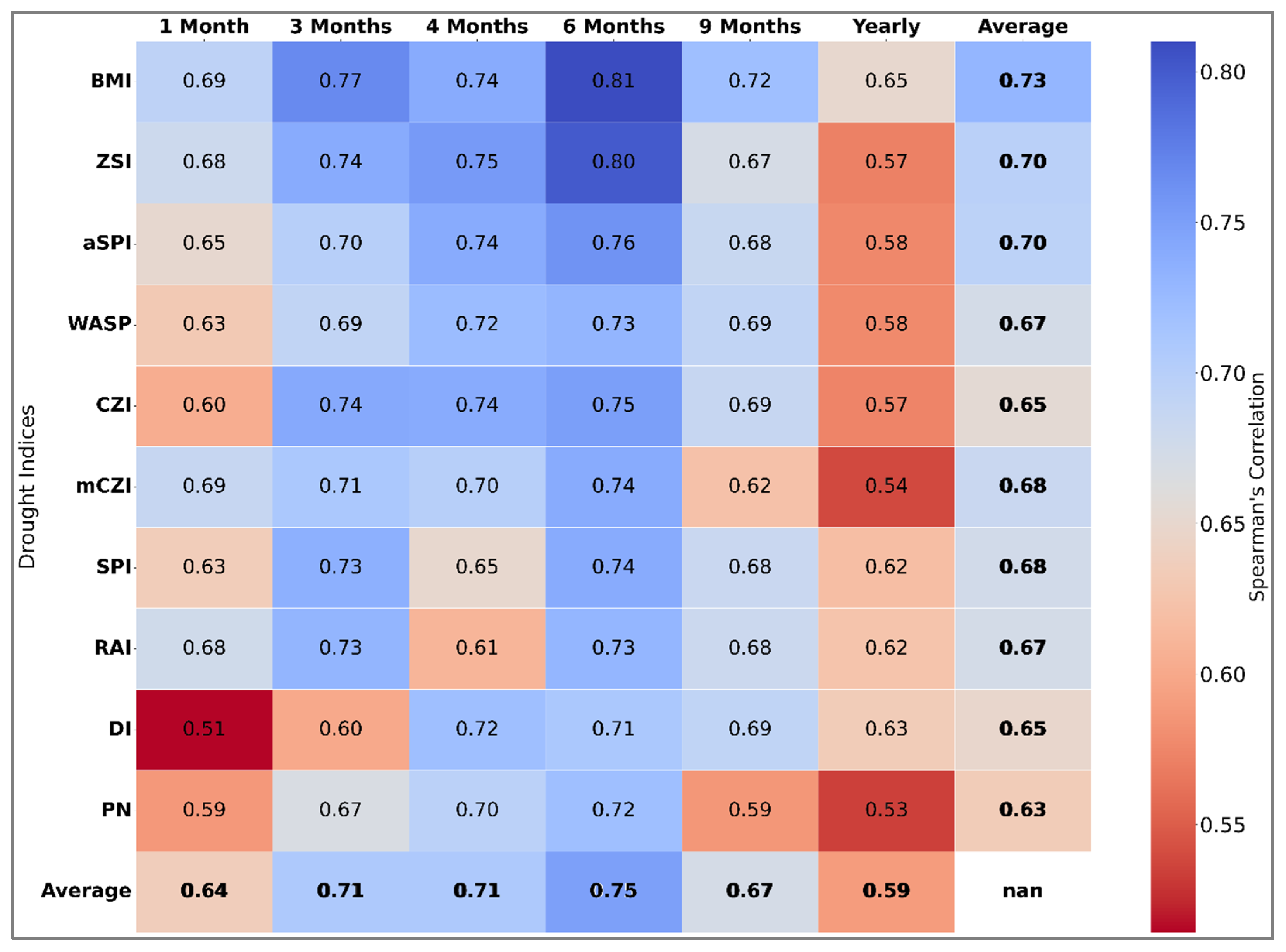
Figure 3 illustrates the comparison of ten drought indices using Spearman’s rank correlation values for different time scales of 1, 3, 4 (starting from June), 6, 9, and 12 months. The indices, such as BMDI, ZSI, and aSPI, revealed the highest average correlations among all the indices (ρ > 0.70) across all timesteps. The persistence of strong positive correlations across various timescales implies a strong dependence structure, indicating similar temporal dynamics of drought patterns based on their strength and similarity. In contrast, lower average correlations (<0.68) were observed for PNI, RAI, and DI, suggesting potential differences in the elements of drought patterns captured by these indices.

Figure 3.
Spearman’s correlation values for different timescales. Bold values denote average correlation across timescales (column) and across indices (row).
Across all timesteps, the average correlation increased steadily from one to six months, reaching its highest value at the half-yearly interval (ρ = 0.75). After six months, there was a gradual decline in correlation values, with the 9-month time scale dropping to 0.67. The annual timescale demonstrated the lowest correlation (ρ = 0.59), followed by a monthly timescale (ρ = 0.64). Similar patterns were observed based on the previous findings for the semi-arid regions of India [,] and Turkey [], where correlations increased from monthly to half-yearly timesteps before declining at 9 and 12 months. This correlation pattern may be due to seasonal variations in TP, particularly during the monsoon months (June–September), which result in substantial hydrological recharge, increased soil moisture, and higher groundwater and water levels. This recharge of water resources reduces the risk of drought in the subsequent months. Additionally, droughts in semi-arid regions often require four to six months to fully develop [], as soil moisture and groundwater recover slowly from earlier precipitation deficits, due to lagged hydrological responses. Hence, monthly timescales may underestimate drought severity and duration due to the inability to incorporate temporal lag hydrological responses, making shorter intervals less efficient for precise drought monitoring. The consistent high correlations at 3-, 4-, and 6-month periods highlight the importance of longer timesteps, as they can better capture the lagged gradual development and persistence of drought events.
Furthermore, water scarcity in Marathwada often arises when monsoon rainfall, particularly from June to August, is below average (negative anomaly). Hence, the persisting water deficits are exacerbated by limited rainfall during the monsoon withdrawal period (September to October), which restricts water resource replenishment. This results in prolonged water shortages and an increased risk of drought, particularly from January to June. These hydrometeorological factors make a 6-month timescale optimal for drought monitoring. These findings contradict previous findings for the 9-month time scale, which was regarded as the optimal time step for drought monitoring in central India []. These differences may be attributed to regional variations in rainfall patterns, evaporation rates, and differing soil properties that influence drought development, as well as the limited number of drought indices used in the earlier study.
Among the drought indices, the BMDI, ZSI, and RAI revealed a higher correlation (ρ > 0.65) at the monthly timescale. At 3- and 4-month time scales, BMI, ZSI, aSPI, and CZI exhibited temporal stability, as indicated by consistent high correlations (ρ > 0.70) with TP variability (Table 4), highlighting their applicability for capturing short-term droughts. SPI demonstrated consistency at the 3-month timescale (ρ = 0.73) but revealed weaker performance at the 4-month timescale (ρ = 0.65) during the monsoon season, which may be attributable to violations of its underlying Gamma distribution assumptions. At a 6-month timescale, BMDI, ZSI, and aSPI exhibited the highest average correlation values (ρ > 0.75), indicating that these indices are temporally consistent and capture similar drought patterns. For long-term droughts at 9 to 12 months, BMI, ZSI, aSPI, WASP, and DI demonstrated greater stability in capturing persistent dry spells compared to other indices. Although a previous study reported strong performance of the Effective Drought Index (EDI) in the semi-arid region of Iran [], the EDI was not computed in the analysis due to limitations in daily based data. Additionally, as Iran does not have a monsoon-dependent climate, direct comparison with the present study’s climatic context is limited. These differences in correlation patterns demonstrate that no single index is universally applicable, emphasizing the need to compare multiple drought indices for robust drought assessment.

Table 4.
Most applicable drought indices across different timescales.
4.4. Evaluation of Drought Indices Using Statistical Performance
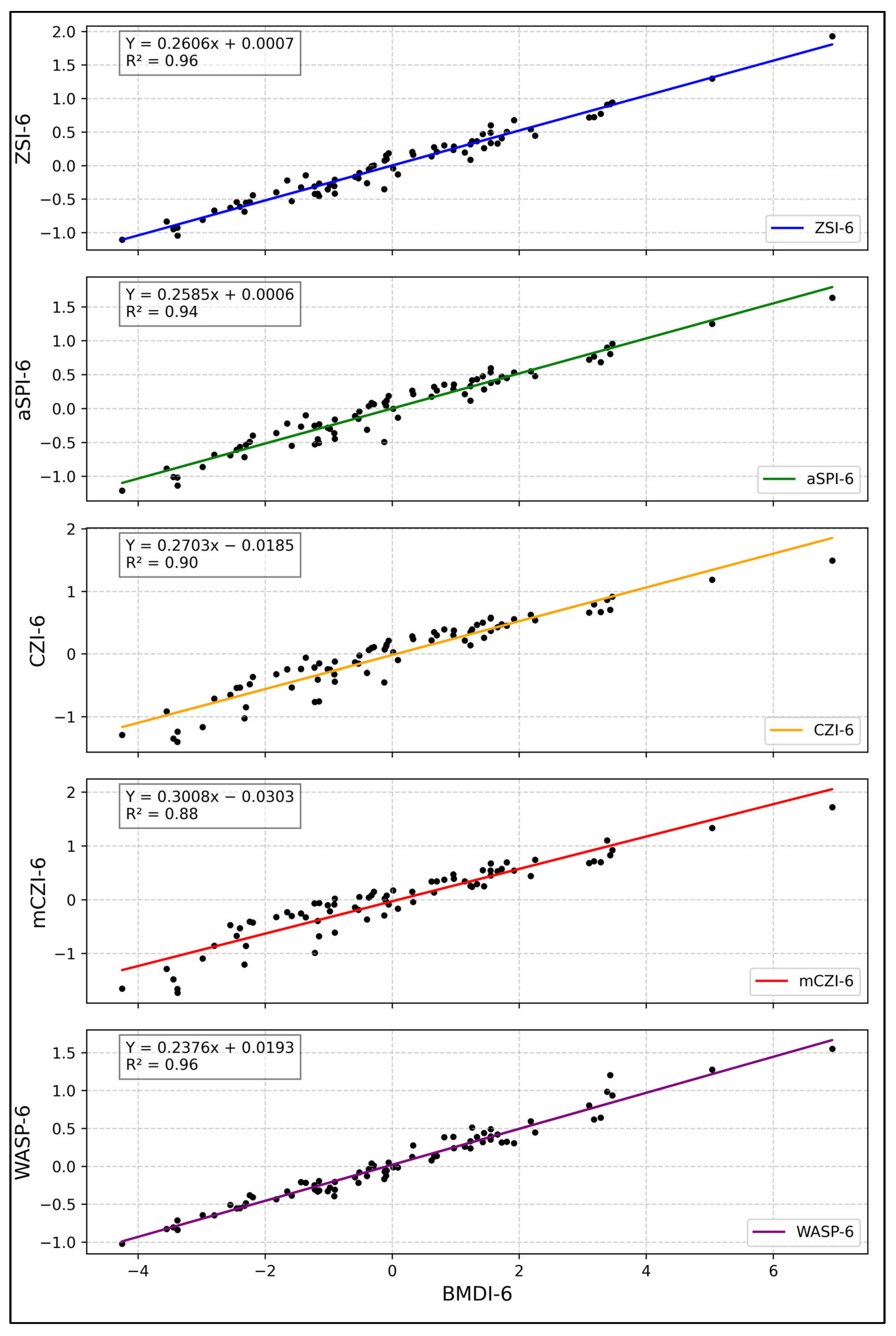
The relationships between BMDI-6 and ZSI-6, aSPI-6, CZI-6, mCZI-6, and, WASP-6 were plotted to evaluate the robustness and sensitivity of drought indices (Figure 4). Although SPI is internationally recognized and frequently used as a reference index, its applicability in semi-arid regions is limited due to violations of the Gamma distribution assumption required for accurate computation []. Hence, a non-parametric-based BMDI-6 was selected as the reference index based on its highest Spearman’s correlation (ρ = 0.75) with other indices, indicating strong temporal consistency. Additionally, BMDI was developed explicitly for monitoring droughts under Indian monsoon conditions, enhancing its regional relevance.

Figure 4.
Linear relationship between the BMDI-6 and other drought indices.
The comparative analysis revealed that aSPI-6, ZSI-6, WASP-6, and CZI-6 exhibited the highest R2 values (>0.97), indicating that these models can explain 97% of the variability in BMDI-6. The lowest RMSE (<0.20) and SEE (<0.20) among these indices demonstrate their hydro-meteorological comparability with BMDI-6 in representing drought severity in detecting prolonged temporal drought patterns. A standard deviation of close to one (Table 5) indicates temporal consistency throughout the 75 years, while higher values imply greater variability in drought patterns. This demonstrates that these indices are temporally stable in capturing drought variability across the study domain.

Table 5.
Statistical criteria to evaluate the performance of drought indices.
Conversely, DI-6 and RAI-6 revealed the lowest coefficients of determination (R2 < 0.58) and the highest RMSE (0.69 and 1.03, respectively). This could be due to DI’s rank-based criteria that classify precipitation into historical percentiles [], making it highly sensitive to local precipitation frequency rather than capturing the cumulative effects of sustained rainfall deficits. Therefore, DI is less effective than anomaly-based indices, such as BMDI, for monitoring prolonged droughts, as revealed by the lower R2 and higher RMSE values. PN-6 also demonstrated the highest RMSE, SEE, SEM, and MAE compared to other indices, indicating poor temporal consistency (temporal instability) with the BMDI-6. This may be attributed to its limited ability to accurately capture seasonal variability, particularly in regions with alternative wet and dry seasons. Hence, these findings suggest that DI-6, RAI-6, and PN-6 are less applicable for precise drought monitoring in Marathwada.
SPI-6 revealed a lower R2 (0.60) and higher RMSE, SEE, SEM, and MAE compared to ZSI-6, WASP-6, CZI-6, and mCZI-6, indicating weaker temporal consistency with observed drought conditions in Marathwada. These findings are consistent with the previous studies of Mwinjuma et al. [] and Nadi et al. [], which reported the limitations of SPI in detecting drought occurrences and severity, particularly for short-term drought monitoring at timescales of less than nine months in semi-arid regions worldwide. This relatively lower performance may be attributed to SPI’s assumption that TP follows a Gamma distribution, which requires a positively skewed, continuous probability distribution. However, several studies have applied SPI using Gamma [], or Pearson type III distribution [] without validating these assumptions with the goodness-of-fit measures. Hence, any violations of SPI’s distributional assumptions can affect SPI’s reliability in regions where precipitation patterns deviate from the assumed distribution, potentially leading to higher error metrics and temporal inconsistencies.
In semi-arid regions such as Marathwada, rainfall is dominated within a few monsoon months (June–September), while most other months remain dry. These seasonal patterns result in zero-inflated TP data in non-monsoon months, leading to geospatial and temporal heterogeneity. Hence, TP distributions exhibit pronounced skewness, and heavy-tailed distributions, leading to asymmetry. As a result, the estimation of the Gamma distribution’s shape (α) and scale (β) parameters becomes unstable and biased [], which can distort the cumulative density functions (CDF), resulting in non-robust SPI values [,].
Consequently, several researchers have proposed alternative distributions, such as Pearson’s Type III, Weibull, and exponential Weibull, to capture the characteristics of TP distributions better [] and improve SPI’s goodness-of-fit []. However, these distributions still assume continuous positively skewed TP data with stable α and β parameters, making them sensitive to deviations caused by zero-inflated TP. While Pearson’s Type III distribution is comparatively more flexible to skewness due to its location (θ) parameter, it assumes unimodality and finite bound conditions, which are violated in the presence of zero-inflated TP data []. This was confirmed by Guttman [], who reported no significant differences in SPI across these distributional choices.
The low R2 with higher error metrics, as revealed by SPI, highlights the inadequacy of relying on parametric assumptions that are violated in the presence of excess kurtosis and skewness in TP []. These distributional assumptions can result in underestimation or misclassification of drought events, particularly in semi-arid to arid regions []. This underscores the need for region-specific, non-parametric alternatives, such as BMDI-6 and ZSI-6. Thus, time series with high temporal skewness and heavy tails can violate the distributional assumptions of the Gamma [] and Pearson’s Type III distribution [], challenging the statistical validity of SPI for precise drought assessment in the study domain.
These limitations not only question the robustness of SPI but also highlight the challenges of developing a composite drought index. The applicability of composite indices could be challenged based on their parametric and non-parametric statistical assumptions. In the semi-arid region of Marathwada, the presence of zero-inflated asymmetric thick-tailed data can violate the Gamma or Pearson Type III distribution. Additionally, combining indices could lead to confounding effects due to a lack of variable-specific weightage or influence (e.g., precipitation, temperature, humidity). Hence, a composite index could reduce interpretability and weaken the region-specific applicability of the results. Thus, indices were evaluated individually to ensure the robustness of both parametric and non-parametric assumptions.
4.5. Evaluation of Drought Indices Using Historical Events
The performance of drought indices was evaluated based on their ability to accurately detect drought onset, termination, and severity. For this analysis, the period from January 1971 to December 1974 was selected as the most prolonged drought in the Marathwada region, as detected by BMDI-6, ZSI-6, aSPI-6, WASP-6, CZI-6, and mCZI-6. A 6-month cumulative TP timescale was employed to evaluate the performance of each drought index to TP deficits (negative TP anomaly). The 6-month cumulative TP for each month was computed as the sum of precipitation of the current and the previous five months, that is, from January to June. Similarly, the 6-monthly average TP was computed as the average of all the specific months in the 6-month cumulative TP. This rolling, 6-monthly cumulative TP approach provides a more accurate reflection of persistent rainfall deficits and their impacts on drought development.
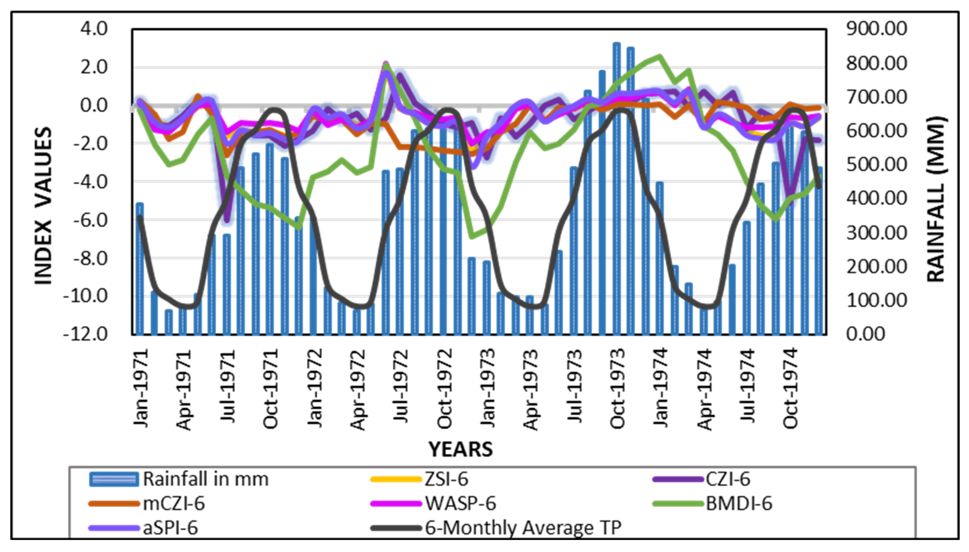
Figure 5 illustrates that January 1971 recorded a surplus of approximately 350 mm of TP. There were no droughts until February 1971, as indicated by the ZSI-6, CZI-6, mCZI-6, WASP-6, and aSPI-6. However, BMDI-6 detected droughts from January to May 1971. This early drought detection by BMDI-6 may reflect the temporal lag effects of the severe drought event in 1969, which resulted in eight consecutive months of drought. Once a drought event is initiated, its termination is not instant, as it requires prolonged periods of above-average TP to overcome the negative TP anomalies []. Although 1970 saw above-average TP (496 mm), this was insufficient to fully overcome the cumulative TP deficits, particularly due to the lower annual averages (400 mm) observed from 1971 to 1974. As a result, drought conditions persisted, despite intermittent rainfall surpluses. This indicates that droughts do not terminate instantly, even with significant rainfall in subsequent months, as they must overcome the previous negative TP anomalies.

Figure 5.
Comparison of Meteorological Drought Indices with Rainfall Deficiencies. BMDI values were classified according to the method described by Bhalme and Mooley []: ≤−4.0 (extreme drought), −3.0 to −3.99 (severe drought), −2.0 to −2.99 (moderate drought), and −1.0 to −1.99 (mild drought).
BMDI-6 detected June 1971 as a temporary escape from drought, likely due to surplus rainfall in May and June. Despite this, the drought persisted from February 1971 to July 1973, marking a 30-month period as the most prolonged drought in Marathwada during the 1971–1973 period. ZSI-6, WASP-6, aSPI-6, CZI-6, and mCZI-6 exhibited similar drought patterns, ranging from moderately dry to severely dry periods (Figure 5), indicating their sensitivity to rainfall deficits. BMDI-6 identified extremely dry conditions (<−4.0) from December 1972 to February 1973, while the other indices indicated moderate to severe dryness for the same period. This demonstrates that BMDI-6 is more sensitive to the rainfall deficit than the other indices. Similar findings were reported by [], who found that BMDI was more sensitive than the Palmer Drought Severity Index (PDSI) in detecting drought patterns in East Africa. This implies BMDI’s efficiency in capturing drought dynamics that extend beyond the Indian monsoon climate, such as the Intertropical Convergence Zone (ITCZ) driven rainfall regime of East Africa. The effectiveness and applicability of BMDI in detecting precise drought patterns can be attributable to its reliance on long-term standardized rainfall anomalies, which enable accurate detection of multiple wet and dry periods within a year.
The period from August 1973 to March 1974, including the monsoon 1973, revealed near-normal conditions across all drought indices due to above-average TP during this period. However, WASP-6 detected drought months from April to September 1974, while BMDI-6 revealed drought conditions extending through December 1974. This indicates that both indices responded promptly to changes in TP anomalies. In contrast, the rest of the indices did not detect any drought conditions until July 1974, indicating a lag in drought detection due to gradual recovery from preceding negative TP anomalies. Hence, a continuous above-average prolonged TP is required to replenish negative TP anomalies. Normal to wet conditions could be reached during the above-average prolonged TP. However, the ability to replenish the previous water deficits depends on the magnitude of previous negative TP anomalies. This demonstrates that monitoring short-term droughts, such as on a monthly or quarterly timescale, could lead to erroneous results due to the inability to incorporate the lag effects. Therefore, a 6-month timescale is more accurate than the other timesteps for precise drought monitoring.
The comparative analysis of drought indices identified the period from February 1971 to July 1973 as the most prolonged drought period, with BMDI emerging as the most sensitive index to TP fluctuations. These results were verified by the District Statistical Handbook, which also reported drought months from February 1971 to July 1973 [].
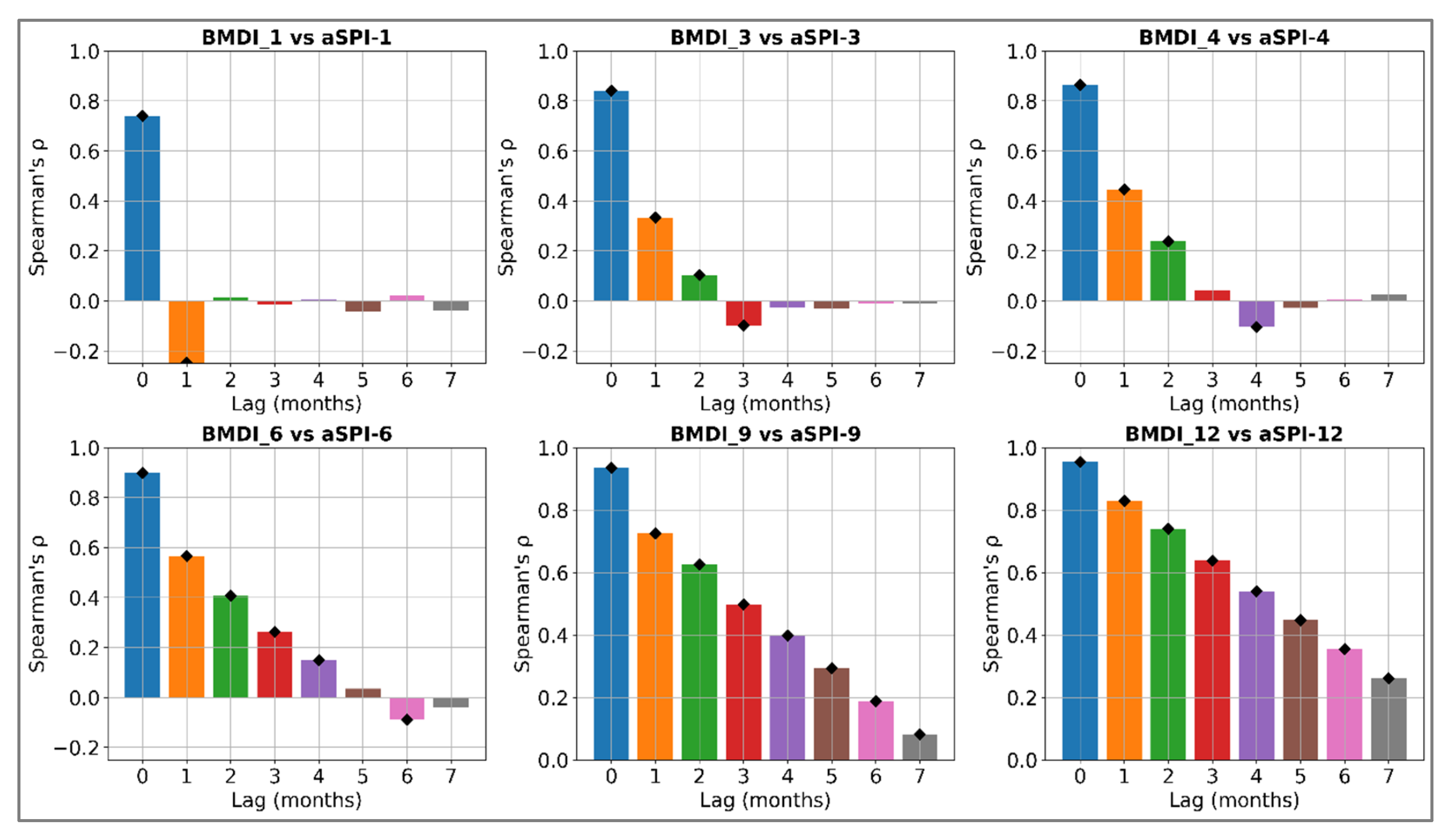
4.6. Time Lag Association Between Meteorological and Agricultural Droughts
The non-linear lag relationship between meteorological (BMDI) and agricultural (aSPI) droughts was evaluated using SCCF at lags of 0 to 7 months (Figure 6), across multiple time scales (1, 3, 4, 6, 9, and 12 months). BMDI was selected as the reference meteorological drought index due to its sensitivity to the semi-arid Indian monsoon climate, as it is specifically developed for monitoring droughts for the Indian monsoon climate []. While SPI is globally recognized, its applicability in the semi-arid Indian monsoon-based climate is limited due to its violations of the gamma distribution assumption. In contrast, BMDI revealed the strongest Spearman correlation in this study, supporting its robustness for evaluating temporal lag relationships with agricultural droughts. aSPI was chosen for its ability to incorporate effective precipitation, considering soil moisture, which is suitable for agricultural drought monitoring.

Figure 6.
Cross-correlation matrix between meteorological and agricultural droughts at different timescales.
For a monthly timestep, SCCF demonstrated no significant lag relationship between BMDI and aSPI, indicating agricultural droughts are not highly sensitive to short-term meteorological droughts. This finding is similar to Wu and Kinter [], who detected weak relationships between meteorological and agricultural droughts at the monthly timescale. In contrast, Salimi et al. [] found that hydrological droughts responded to meteorological droughts with lags of up to two months in a hot, arid region of Iran, compared to Marathwada, which is characterized by a non-monsoon-based climate.
Regions with poor soil water retention or shallow soils often experience rapid declines in soil moisture following TP deficits. In such environments, especially in arid to semi-arid areas with high evapotranspiration, the effects of meteorological drought can be observed almost instantly in agricultural systems [,]. However, at 3- and 4-month time scales, SCCF revealed a statistically significant lag relationship (p-value < 0.05) at lag 1 (ρ = 0.40), indicating a weak lagged relationship between meteorological and agricultural droughts at shorter time scales.
Across all time scales, SCCF indicated a gradual decline in correlation with increasing lags up to seven months. At a 6-month timestep, SCCF revealed a statistically significant moderate correlation (ρ ≈ 0.5) at lags one and two months, and a weaker but significant correlation (ρ ≈ 0.2) up to four months. This indicates a lagged association between meteorological and agricultural droughts up to four months at a half-yearly timescale. These findings are consistent with the study of Pachore et al. [], who reported a drought propagation time of 4–5 months in the semi-arid region of Maharashtra, central India, and a slightly longer lag of up to 6 months in the arid region of Rajasthan. Similarly, the higher timescales of 9 and 12 months revealed a significant and strong correlation (ρ ≈ 0.7) at lags of up to two months. Although correlation gradually decreases at higher lags beyond one month, a significant lagged relationship was detected up to seven months. These patterns may be attributed to the prolonged impact of meteorological drought on agricultural systems, resulting in extended recovery times from soil moisture deficits, high temperatures, and increased solar radiation, especially in hot, semi-arid regions. These findings are in alignment with previous studies of Torelló-Sentelles and Franzke [] and Zhang et al. [], which highlight stronger and more persistent lag relationships between meteorological and agricultural droughts at longer timescales.
Hence, SCCF revealed a robust non-linear time-lag relationship between meteorological and agricultural droughts, demonstrating that simple linear models may be insufficient to fully capture the complex drought propagation patterns. The previous studies [,,] reported similar limitations that analyzed the relationship between meteorological and hydrological droughts, further emphasizing the need for non-parametric approaches to capture non-linear temporal lag drought propagation patterns.
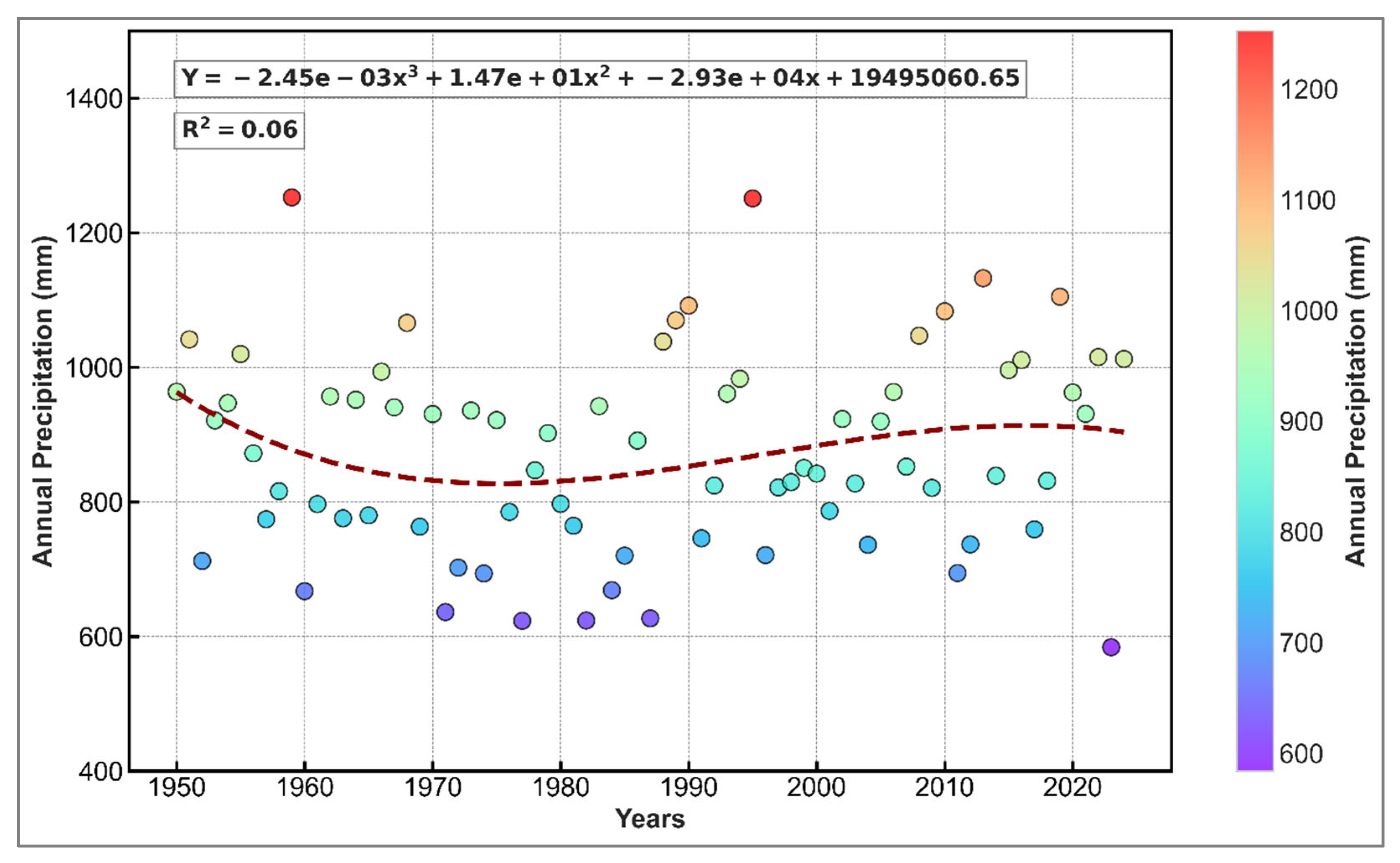
4.7. Annual and Decadal Trends in Total Precipitation
Figure 7 illustrates the time series of total annual precipitation, fitted with a third-order polynomial trend line. The low R2 value of 0.06 demonstrates that the model explains only 6% of the total variability in annual TP. This may be associated with the high interannual and seasonal variability of the monsoon-dependent, semi-arid climate of Marathwada. The trend analysis revealed a gradual decline in TP from 1950 to 1970, with the lowest TP observed during the 1970–80 decade. Consequently, Marathwada experienced its most prolonged droughts during this decade, associated with persistent negative TP anomalies.

Figure 7.
Time series of annual total precipitation from 1951 to 2024. The dotted line represents the third-order polynomial trendline, highlighting long-term annual variability in precipitation.
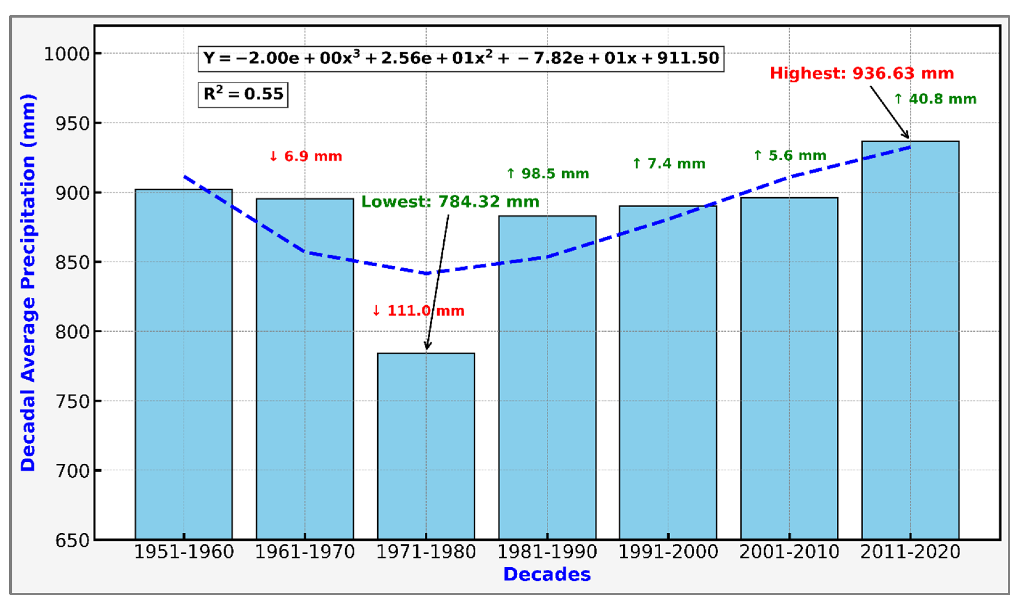
Similarly, Figure 8 depicts the decadal time series of TP from 1951 to 2020, fitted with a third-order polynomial trend line. A slightly better R2 value of 0.55, as compared to annual TP, indicates that the model reveals around 55% of TP variability, suggesting a better fit at the decadal scale. The figure illustrates a steady decline in TP from 1951 to 1980, with the lowest average TP (784 mm) recorded during the 1971–1980 period, which is consistent with Marathwada’s most prolonged drought of that decade. From 1981 to 2020, a gradual increase in TP was observed, indicating a partial recovery from prolonged drought conditions. Despite this increasing trend, drought events have been observed in recent years due to continued high interannual temperature variability, resulting in recurring negative temperature anomalies.

Figure 8.
Time series of decadal total precipitation from 1951 to 2020. The dotted blue line represents the third-order polynomial trendline, highlighting long-term decadal variability in precipitation.
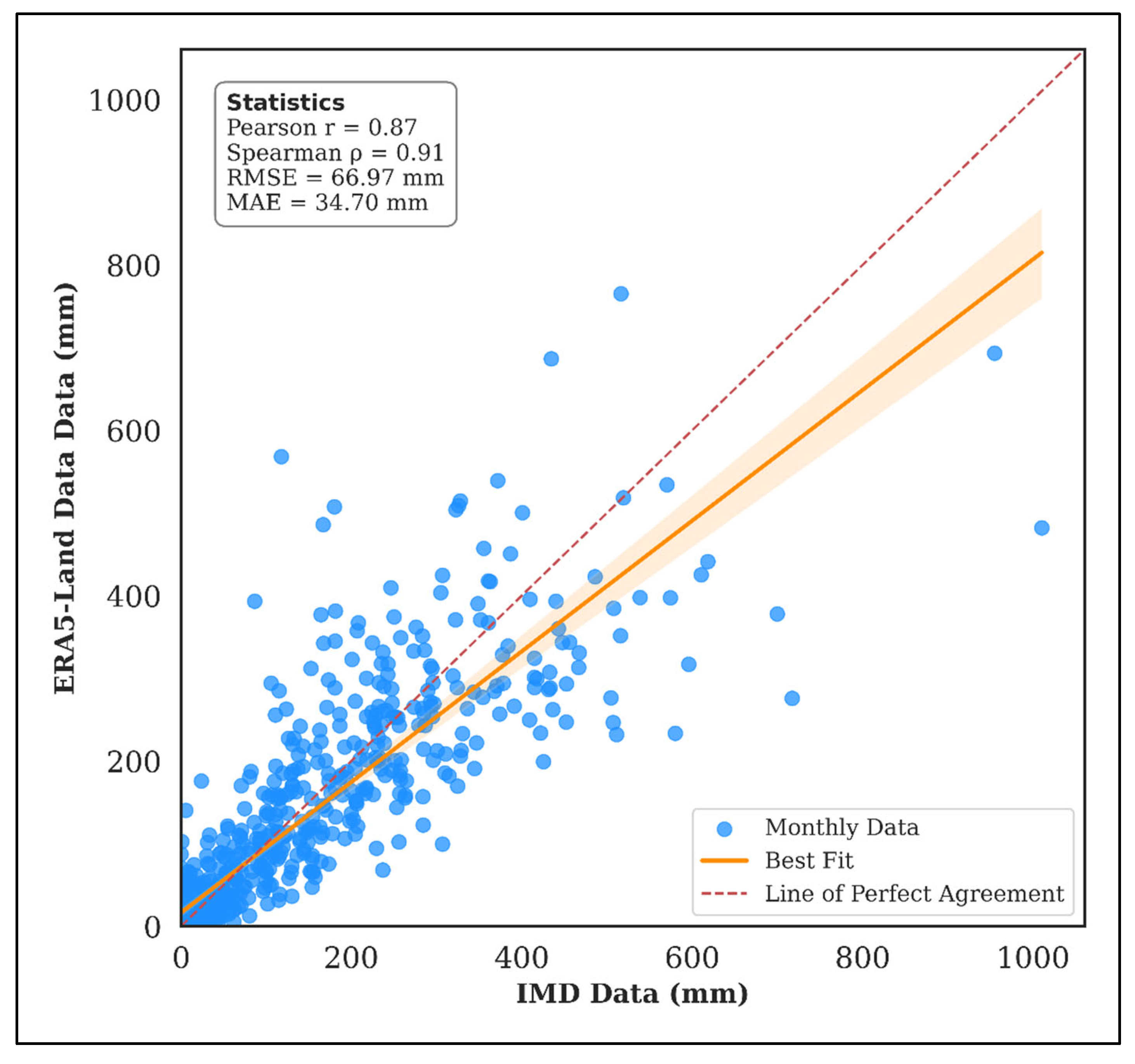
The ERA5-Land-based TP data were validated against the IMD data by re-gridding with IMD’s 0.5° latitude by 0.5° longitude resolution and validated over the Marathwada region. The results revealed a robust temporal consistency, with Pearson’s r (0.87) and Spearman’s ρ (0.91) with a p-value < 0.001 (Figure 9). This indicates that ERA5-Land effectively captured both linear and non-linear TP seasonal variability. Additionally, the error metrics revealed a lower RMSE (66.97 mm), MAE (34.70), and MBE (−3.01 mm), demonstrating temporal stability with minimal bias. The KGE (0.83) further demonstrated an agreement with the ERA5-Land and IMD datasets by incorporating accurate TP amounts, variability, and temporal patterns. Hence, these results indicate that ERA5-Land provides an accurate TP estimate consistent with IMD observations, justifying its usage for drought assessment in Marathwada, where meteorological ground-based stations are limited.

Figure 9.
Scatterplot of IMD and ERA5-Land Data.
Understanding long-term trends in TP and drought patterns can provide valuable insights for assessing the relationship between climate variability and drought impacts, as well as detecting drought antecedents within the hydrometeorological context. As Marathwada is predominantly agricultural, the cold spots in TP areas can be prioritized for irrigation planning, the adoption of drought-resilient crop varieties, and the modification of crop planting schedules through early warning interventions. Conversely, hot spot zones of TP can be strategized for water harvesting, groundwater recharge, and dam construction to mitigate future drought conditions. Furthermore, the timing and targeting of critical drought interventions can be integrated into social messaging platforms to inform farmers about optimal crop planting and harvesting times, as well as drought-related medical preparedness, particularly during heatwaves. These timely communications can help farmers make climate-informed decisions, thereby increasing the chances of higher crop yields and reducing economic losses.
5. Conclusions
This study addressed key research gaps by identifying the most applicable drought indices for accurate regional drought monitoring in the semi-arid region of Marathwada. Comparative analysis of sGARCH (1,1) and eGARCH (1,1) models revealed that eGARCH (1,1) with a skewed Student’s t distribution was the most optimal for detecting temporal volatility in the TP dataset. The eGARCH (1,1) model demonstrated a lower, non-significant chi-square statistic (17.07), compared to the higher, significant chi-square statistic of sGARCH (70.35), indicating the robustness of eGARCH in modeling non-stationary heteroscedastic time series TP data.
The performance of continuous drought indices data was evaluated using non-parametric Spearman’s correlation to assess the strength, direction, and similarity of regional-specific drought events. The results revealed that the six-month timescale exhibited the highest correlation (ρ = 0.75), whereas the monthly timescale indicated the lowest correlation (ρ = 0.64). The findings demonstrated that droughts develop gradually over time, and hence, monitoring droughts on a monthly timescale may lead to an erroneous assessment due to their inability to capture long-term temporal lags within a month. BMDI-6, ZSI-6, and aSPI-6 demonstrated the highest average correlation (ρ = 0.70), while PNI-6, RAI-6, and DI-6 indicated the lowest (ρ ≤ 0.70). BMDI-6 and WASP-6 were found to be the most sensitive to TP fluctuations, thereby detecting drought events more precisely than the other indices. The historical drought analysis revealed the period from February 1971 to July 1973 as the most prolonged drought, associated with the lowest TP during the 1970–1980 decade. Although SPI is globally recognized and has widespread applicability, its performance in the semi-arid region was not optimal due to the violations of Gamma distribution assumptions resulting from zero-inflated TP data. Hence, non-parametric indices like BMDI-6, ZSI-6, and WASP-6 are recommended for drought monitoring in the Marathwada region. Spearman’s cross-correlation further revealed that meteorological droughts did not influence agricultural droughts at the monthly timescale. However, significant lagged relationships emerged at 6-, 9-, and 12-month timescales, with temporal lags of up to four months.
This study is limited by its reliance on precipitation-based drought indices and the absence of soil moisture validation using remote sensing data, which may impact the precision of agricultural drought assessment. Thus, future work could strengthen these findings by incorporating high-resolution vegetation- and water-based remote sensing indices, along with land-use/land-cover and topographical datasets, such as elevation. Integrating soil moisture estimates would further strengthen the validation of agricultural drought assessments by detecting soil moisture deficits that affect crop productivity. Additionally, incorporating future Community Earth System Model (CESM) projections under different Representative Concentration Pathways (RCPs) and Shared Socioeconomic Pathways (SSPs) would provide deeper insights into the geospatial and temporal evolution of drought patterns under changing climate scenarios.
Supplementary Materials
The following supporting information can be downloaded at https://www.mdpi.com/article/10.3390/hydrology12100254/s1, Table S1: Drought Classification of BMI; Table S2: Drought Classification of ZSI, aSPI, CZI, mCZI, and WASP.
Author Contributions
N.C., B.G.J., Y.E. and J.C. contributed to the study’s conception and design. N.C. performed material preparation, data collection, and analysis. B.G.J., Y.E. and J.C. contributed to the study’s conception, supervision, and revision. B.G.J., Y.E. and J.C. reviewed and edited the manuscript. All authors have read and agreed to the published version of the manuscript.
Funding
This research received no external funding.
Data Availability Statement
The data presented in this study are available upon request from the corresponding author.
Acknowledgments
We would like to thank Dominic Del Pino for reviewing the paper and Dilip Panchamia for validating the drought indices output.
Conflicts of Interest
The authors declare no conflicts of interest.
References
- Dracup, J.A.; Lee, K.S.; Paulson, E.G., Jr. On the definition of droughts. Water Resour. Res. 1980, 16, 297–302. [Google Scholar] [CrossRef]
- Ding, Y.; Xu, J.; Wang, X.; Peng, X.; Cai, H. Spatial and temporal effects of drought on Chinese vegetation under different coverage levels. Sci. Total Environ. 2020, 716, 137166. [Google Scholar] [CrossRef]
- Wang, T.; Tu, X.; Singh, V.P.; Chen, X.; Lin, K.; Zhou, Z.; Tan, Y. Assessment of future socioeconomic drought based on CMIP6: Evolution, driving factors and propagation. J. Hydrol. 2023, 617, 129009. [Google Scholar] [CrossRef]
- Wilhite, D.A. Drought as a natural hazard: Concepts and definitions. In Droughts; Routledge: Oxfordshire, UK, 2016; pp. 3–18. [Google Scholar]
- Ma, S.; Zhang, S.; Wang, N.; Huang, C.; Wang, X. Prolonged duration and increased severity of agricultural droughts during 1978 to 2016 detected by ESA CCI SM in the humid Yunnan Province, Southwest China. Catena 2021, 198, 105036. [Google Scholar] [CrossRef]
- Zhang, L.; Jiao, W.; Zhang, H.; Huang, C.; Tong, Q. Studying drought phenomena in the Continental United States in 2011 and 2012 using various drought indices. Remote Sens. Environ. 2017, 190, 96–106. [Google Scholar] [CrossRef]
- Adnan, S.; Ullah, K.; Shuanglin, L.; Gao, S.; Khan, A.H.; Mahmood, R. Comparison of various drought indices to monitor drought status in Pakistan. Clim. Dyn. 2018, 51, 1885–1899. [Google Scholar] [CrossRef]
- Mishra, V.; Aadhar, S.; Mahto, S.S. Anthropogenic warming and intraseasonal summer monsoon variability amplify the risk of future flash droughts in India. npj Clim. Atmos. Sci. 2021, 4, 1. [Google Scholar] [CrossRef]
- Mahto, S.S.; Mishra, V. Dominance of summer monsoon flash droughts in India. Environ. Res. Lett. 2020, 15, 104061. [Google Scholar] [CrossRef]
- Svoboda, M.D.; Fuchs, B.A. Handbook of Drought Indicators and Indices; World Meteorological Organization: Geneva, Switzerland, 2016; Volume 2. [Google Scholar]
- Huang, K.; Wu, J.; Fu, Z.; Du, J. Comparative analysis of drought indices in the tropical zones of China. Sci. Total Environ. 2024, 947, 174530. [Google Scholar] [CrossRef]
- Alahacoon, N.; Edirisinghe, M. A comprehensive assessment of remote sensing and traditional based drought monitoring indices at global and regional scale. Geomat. Nat. Hazards Risk 2022, 13, 762–799. [Google Scholar] [CrossRef]
- Pan, Y.; Zhu, Y.; Lue, H.; Yagci, A.L.; Fu, X.; Liu, E.; Xu, H.; Ding, Z.; Liu, R. Accuracy of agricultural drought indices and analysis of agricultural drought characteristics in China between 2000 and 2019. Agric. Water Manag. 2023, 283, 108305. [Google Scholar] [CrossRef]
- Pathak, A.A.; Dodamani, B. Comparison of meteorological drought indices for different climatic regions of an Indian river basin. Asia-Pac. J. Atmos. Sci. 2020, 56, 563–576. [Google Scholar] [CrossRef]
- Uddin, M.A.; Kamal, A.M.; Shahid, S.; Chung, E.-S. Volatility in rainfall and predictability of droughts in northwest Bangladesh. Sustainability 2020, 12, 9810. [Google Scholar] [CrossRef]
- Bouznad, I.-E.; Guastaldi, E.; Zirulia, A.; Brancale, M.; Barbagli, A.; Bengusmia, D. Trend analysis and spatiotemporal prediction of precipitation, temperature, and evapotranspiration values using the ARIMA models: Case of the Algerian Highlands. Arab. J. Geosci. 2020, 13, 1281. [Google Scholar] [CrossRef]
- Ghosh, S.; Mukhoti, S.; Sharma, P. Quantifying rainfall-induced climate risk in rainfed agriculture: A volatility-based time series study from semi-arid India. Agric. Water Manag. 2025, 319, 109775. [Google Scholar] [CrossRef]
- Tijdeman, E.; Stahl, K.; Tallaksen, L.M. Drought characteristics derived based on the standardized streamflow index: A large sample comparison for parametric and nonparametric methods. Water Resour. Res. 2020, 56, e2019WR026315. [Google Scholar] [CrossRef]
- Pandya, P.A.; Gontia, N.K. Correlation vs. Kappa statistic: A new perspective on comparing meteorological drought indices. Theor. Appl. Climatol. 2025, 156, 19. [Google Scholar] [CrossRef]
- Vergni, L.; Todisco, F.; Di Lena, B. Evaluation of the similarity between drought indices by correlation analysis and Cohen’s Kappa test in a Mediterranean area. Nat. Hazards 2021, 108, 2187–2209. [Google Scholar] [CrossRef]
- Bilal, S.B.; Gupta, V. Deciphering the spatial fingerprint of drought propagation through precipitation, vegetation and groundwater. Int. J. Climatol. 2024, 44, 4443–4461. [Google Scholar] [CrossRef]
- Xu, Z.; Wu, Z.; Shao, Q.; He, H.; Guo, X. From meteorological to agricultural drought: Propagation time and probabilistic linkages. J. Hydrol. Reg. Stud. 2023, 46, 101329. [Google Scholar] [CrossRef]
- Ogunrinde, A.T.; Adigun, P.; Xue, X.; Koji, D.; Jing, Q. Spatiotemporal analysis of drought patterns and trends across Africa: A multi-scale SPEI approach (1960–2018). Int. J. Digit. Earth 2025, 18, 2447342. [Google Scholar] [CrossRef]
- Raziei, T.; Pereira, L.S. Relating the drought precipitation percentiles index to the standardized precipitation index (SPI) under influence of aridity and timescale. Water Resour. Manag. 2024, 38, 5739–5758. [Google Scholar] [CrossRef]
- Terzi, T.B.; Önöz, B. Drought analysis in the Seyhan River Basin based on standardized drought indices using a new approach considering seasonality. Environ. Earth Sci. 2025, 84, 30. [Google Scholar] [CrossRef]
- Öz, F.Y.; Özelkan, E.; Tatlı, H. Comparative analysis of SPI, SPEI, and RDI indices for assessing spatio-temporal variation of drought in Türkiye. Earth Sci. Inform. 2024, 17, 4473–4505. [Google Scholar] [CrossRef]
- Rogelj, J.; Luderer, G.; Pietzcker, R.C.; Kriegler, E.; Schaeffer, M.; Krey, V.; Riahi, K. Energy system transformations for limiting end-of-century warming to below 1.5 C. Nat. Clim. Change 2015, 5, 519–527. [Google Scholar] [CrossRef]
- Srivastava, A.; Maity, R. Unveiling an Environmental Drought Index and its applicability in the perspective of drought recognition amidst climate change. J. Hydrol. 2023, 627, 130462. [Google Scholar] [CrossRef]
- McKee, T.B.; Doesken, N.J.; Kleist, J. The relationship of drought frequency and duration to time scales. In Proceedings of the 8th Conference on Applied Climatology, Anaheim, CA, USA, 17–22 January 1993; pp. 179–183. [Google Scholar]
- Dogan, S.; Berktay, A.; Singh, V.P. Comparison of multi-monthly rainfall-based drought severity indices, with application to semi-arid Konya closed basin, Turkey. J. Hydrol. 2012, 470, 255–268. [Google Scholar] [CrossRef]
- Li, L.; Cai, H. A comparative study of various drought indices at different timescales and over different record lengths in the arid area of northwest China. Environ. Sci. Pollut. Res. 2024, 31, 25096–25113. [Google Scholar] [CrossRef] [PubMed]
- Bhalme, H.N.; Mooley, D.A. Large-scale droughts/floods and monsoon circulation. Mon. Weather Rev. 1980, 108, 1197–1211. [Google Scholar] [CrossRef]
- Kumar, V.; Chu, H.-J. Spatiotemporal consistency and inconsistency of meteorological and agricultural drought identification: A case study of India. Remote Sens. Appl. Soc. Environ. 2024, 33, 101134. [Google Scholar] [CrossRef]
- Pividori, M.; Ritchie, M.D.; Milone, D.H.; Greene, C.S. An efficient, not-only-linear correlation coefficient based on clustering. Cell Syst. 2024, 15, 854–868.e3. [Google Scholar] [CrossRef]
- Abu Arra, A.; Şişman, E. New Insights into Meteorological and Hydrological Drought Modeling: A Comparative Analysis of Parametric and Non-Parametric Distributions. Atmosphere 2025, 16, 846. [Google Scholar] [CrossRef]
- Xu, L.; Zhang, X.; Yu, H.; Chen, Z.; Du, W.; Chen, N. Incorporating spatial autocorrelation into deformable ConvLSTM for hourly precipitation forecasting. Comput. Geosci. 2024, 184, 105536. [Google Scholar] [CrossRef]
- Khoorani, A.; Balaghi, S.; Mohammadi, F. Projecting drought trends and hot spots across Iran. Nat. Hazards 2024, 120, 9489–9502. [Google Scholar] [CrossRef]
- Griffith, D.A. Spatial filtering. In Spatial Autocorrelation and Spatial Filtering: Gaining Understanding Through Theory and Scientific Visualization; Springer: Berlin/Heidelberg, Germany, 2003; pp. 91–130. [Google Scholar]
- Kwon, M.; Sung, J.H. Changes in future drought with HadGEM2-AO projections. Water 2019, 11, 312. [Google Scholar] [CrossRef]
- Pieper, P.; Düsterhus, A.; Baehr, J. A universal Standardized Precipitation Index candidate distribution function for observations and simulations. Hydrol. Earth Syst. Sci. 2020, 24, 4541–4565. [Google Scholar] [CrossRef]
- Romero, D.; Alfaro, E.J. Systematic Biases in Tropical Drought Monitoring: Rethinking SPI Application in Mesoamerica’s Humid Regions. Meteorology 2025, 4, 18. [Google Scholar] [CrossRef]
- Cammalleri, C.; Spinoni, J.; Barbosa, P.; Toreti, A.; Vogt, J.V. The effects of non-stationarity on SPI for operational drought monitoring in Europe. Int. J. Climatol. 2022, 42, 3418–3430. [Google Scholar] [CrossRef]
- Lisonbee, J.; Nielsen-Gammon, J.; Trewin, B.; Follingstad, G.; Parker, B. Drought assessment in a changing climate: A review of climate normals for drought indices. J. Appl. Serv. Clim. 2024, 2024, 1–17. [Google Scholar] [CrossRef]
- Bollerslev, T. Generalized autoregressive conditional heteroskedasticity. J. Econom. 1986, 31, 307–327. [Google Scholar] [CrossRef]
- Karami, M.; Shabanlou, S.; Mazaheri, H.; Mokhtari, S.; Najarchi, M. Integration of the Non-linear Time Series GARCH Model with Fuzzy Model Optimized with Water Cycle Algorithm for River Streamflow Forecasting. Int. J. Comput. Intell. Syst. 2024, 17, 156. [Google Scholar] [CrossRef]
- Wang, W.; Wang, J.; Romanowicz, R. Uncertainty in SPI calculation and its impact on drought assessment in different climate regions over China. J. Hydrometeorol. 2021, 22, 1369–1383. [Google Scholar] [CrossRef]
- Madadgar, S.; Moradkhani, H. Spatio-temporal drought forecasting within Bayesian networks. J. Hydrol. 2014, 512, 134–146. [Google Scholar] [CrossRef]
- Tobler, W.R. A computer movie simulating urban growth in the Detroit region. Econ. Geogr. 1970, 46, 234–240. [Google Scholar] [CrossRef]
- Kottek, M.; Grieser, J.; Beck, C.; Rudolf, B.; Rubel, F. World map of the Köppen-Geiger climate classification updated. Meteorol. Z. 2006, 15, 259–263. [Google Scholar] [CrossRef]
- Muñoz-Sabater, J.; Dutra, E.; Agustí-Panareda, A.; Albergel, C.; Arduini, G.; Balsamo, G.; Boussetta, S.; Choulga, M.; Harrigan, S.; Hersbach, H. ERA5-Land: A state-of-the-art global reanalysis dataset for land applications. Earth Syst. Sci. Data 2021, 13, 4349–4383. [Google Scholar] [CrossRef]
- Jones, P.W. First-and second-order conservative remapping schemes for grids in spherical coordinates. Mon. Weather Rev. 1999, 127, 2204–2210. [Google Scholar] [CrossRef]
- Pai, D.; Rajeevan, M.; Sreejith, O.; Mukhopadhyay, B.; Satbha, N. Development of a new high spatial resolution (0.25 × 0.25) long period (1901–2010) daily gridded rainfall data set over India and its comparison with existing data sets over the region. Mausam 2014, 65, 1–18. [Google Scholar] [CrossRef]
- Getis, A.; Griffith, D.A. Comparative spatial filtering in regression analysis. Geogr. Anal. 2002, 34, 130–140. [Google Scholar] [CrossRef]
- Getis, A.; Ord, J.K. The analysis of spatial association by use of distance statistics. Geogr. Anal. 1992, 24, 189–206. [Google Scholar] [CrossRef]
- Box, G.E.; Jenkins, G.M.; Reinsel, G.C.; Ljung, G.M. Time Series Analysis: Forecasting and Control; John Wiley & Sons: Hoboken, NJ, USA, 2015. [Google Scholar]
- Spearman, C. The Proof and Measurement of Association between Two Things. Am. J. Psychol. 1904, 15, 72–101. [Google Scholar] [CrossRef]
- Engle, R.F. Autoregressive conditional heteroscedasticity with estimates of the variance of United Kingdom inflation. Econom. J. Econom. Soc. 1982, 50, 987–1007. [Google Scholar] [CrossRef]
- Dickey, D.A.; Fuller, W.A. Distribution of the estimators for autoregressive time series with a unit root. J. Am. Stat. Assoc. 1979, 74, 427–431. [Google Scholar]
- Sjölander, P. A stationary unbiased finite sample ARCH-LM test procedure. Appl. Econ. 2011, 43, 1019–1033. [Google Scholar] [CrossRef]
- Ljung, G.M.; Box, G.E. On a measure of lack of fit in time series models. Biometrika 1978, 65, 297–303. [Google Scholar] [CrossRef]
- Jarque, C.M.; Bera, A.K. Efficient tests for normality, homoscedasticity and serial independence of regression residuals. Econ. Lett. 1980, 6, 255–259. [Google Scholar] [CrossRef]
- Ampadu, S.; Mensah, E.T.; Aidoo, E.N.; Boateng, A.; Maposa, D. A comparative study of error distributions in the GARCH model through a Monte Carlo simulation approach. Sci. Afr. 2024, 23, e01988. [Google Scholar] [CrossRef]
- Dormann, C.F.; Elith, J.; Bacher, S.; Buchmann, C.; Carl, G.; Carré, G.; Marquéz, J.R.G.; Gruber, B.; Lafourcade, B.; Leitão, P.J. Collinearity: A review of methods to deal with it and a simulation study evaluating their performance. Ecography 2013, 36, 27–46. [Google Scholar] [CrossRef]
- Liu, X.; Yu, S.; Yang, Z.; Dong, J.; Peng, J. The first global multi-timescale daily SPEI dataset from 1982 to 2021. Sci. Data 2024, 11, 223. [Google Scholar] [CrossRef]
- Zhan, C.; Liang, C.; Zhao, L.; Jiang, S.; Zhang, Y. Differential responses of crop yields to multi-timescale drought in mainland China: Spatiotemporal patterns and climate drivers. Sci. Total Environ. 2024, 906, 167559. [Google Scholar] [CrossRef] [PubMed]
- Choi, M.; Jacobs, J.M.; Anderson, M.C.; Bosch, D.D. Evaluation of drought indices via remotely sensed data with hydrological variables. J. Hydrol. 2013, 476, 265–273. [Google Scholar] [CrossRef]
- Oyounalsoud, M.S.; Abdallah, M.; Yilmaz, A.G.; Siddique, M.; Atabay, S. A new meteorological drought index based on fuzzy logic: Development and comparative assessment with conventional drought indices. J. Hydrol. 2023, 619, 129306. [Google Scholar] [CrossRef]
- Tian, Y.; Xu, Y.-P.; Wang, G. Agricultural drought prediction using climate indices based on Support Vector Regression in Xiangjiang River basin. Sci. Total Environ. 2018, 622, 710–720. [Google Scholar] [CrossRef]
- Jain, V.K.; Pandey, R.P.; Jain, M.K.; Byun, H.-R. Comparison of drought indices for appraisal of drought characteristics in the Ken River Basin. Weather Clim. Extrem. 2015, 8, 1–11. [Google Scholar] [CrossRef]
- Wable, P.S.; Jha, M.K.; Shekhar, A. Comparison of drought indices in a semi-arid river basin of India. Water Resour. Manag. 2019, 33, 75–102. [Google Scholar] [CrossRef]
- Willmott, C.J. Some comments on the evaluation of model performance. Bull. Am. Meteorol. Soc. 1982, 63, 1309–1313. [Google Scholar] [CrossRef]
- Willmott, C.J.; Wicks, D.E. An empirical method for the spatial interpolation of monthly precipitation within California. Phys. Geogr. 1980, 1, 59–73. [Google Scholar] [CrossRef]
- Khooriphan, W.; Niwitpong, S.-A.; Niwitpong, S. Bayesian estimation of rainfall dispersion in Thailand using gamma distribution with excess zeros. PeerJ 2022, 10, e14023. [Google Scholar] [CrossRef] [PubMed]
- Sienz, F.; Bothe, O.; Fraedrich, K. Monitoring and quantifying future climate projections of dryness and wetness extremes: SPI bias. Hydrol. Earth Syst. Sci. 2012, 16, 2143–2157. [Google Scholar] [CrossRef]
- Cerpa Reyes, L.J.; Ávila Rangel, H.; Herazo, L.C.S. Adjustment of the standardized precipitation index (SPI) for the evaluation of drought in the arroyo pechelín basin, Colombia, under zero monthly precipitation conditions. Atmosphere 2022, 13, 236. [Google Scholar] [CrossRef]
- De Burgh-Day, C.; Dillon, F. A Hybrid Parametrisation for Precipitation Probability of Exceedance Data; Australian Bureau of Meteorology: Melbourne, Australia, 2021.
- Haight, F.A. Handbook of the Poisson Distribution; Wiley: Hoboken, NJ, USA, 1967. [Google Scholar]
- Goodman, L.A. The multivariate analysis of qualitative data: Interactions among multiple classifications. J. Am. Stat. Assoc. 1970, 65, 226–256. [Google Scholar] [CrossRef]
- Gelman, A. Analysis of variance—Why it is more important than ever. Ann. Stat. 2005, 33, 1–53. [Google Scholar] [CrossRef]
- Pearson, K. VII. Note on regression and inheritance in the case of two parents. Proc. R. Soc. Lond. 1895, 58, 240–242. [Google Scholar] [CrossRef]
- Hauke, J.; Kossowski, T. Comparison of values of Pearson’s and Spearman’s correlation coefficients on the same sets of data. Quaest. Geogr. 2011, 30, 87–93. [Google Scholar] [CrossRef]
- Tigkas, D.; Vangelis, H.; Tsakiris, G. Drought characterisation based on an agriculture-oriented standardised precipitation index. Theor. Appl. Climatol. 2019, 135, 1435–1447. [Google Scholar] [CrossRef]
- Chang, D.; Li, S.; Lai, Z. Effects of extreme precipitation intensity and duration on the runoff and nutrient yields. J. Hydrol. 2023, 626, 130281. [Google Scholar] [CrossRef]
- Ghasempour, R.; Roushangar, K.; Alizadeh, F. Hybrid models for drought forecasting: Integration of multi pre-processing-data driven approaches and non-linear GARCH time series model. Arab. J. Geosci. 2023, 16, 361. [Google Scholar] [CrossRef]
- Modarres, R.; Ouarda, T.B. Modelling heteroscedasticty of streamflow times series. Hydrol. Sci. J. 2013, 58, 54–64. [Google Scholar] [CrossRef]
- Salehnia, N.; Alizadeh, A.; Sanaeinejad, H.; Bannayan, M.; Zarrin, A.; Hoogenboom, G. Estimation of meteorological drought indices based on AgMERRA precipitation data and station-observed precipitation data. J. Arid Land 2017, 9, 797–809. [Google Scholar] [CrossRef]
- Spinoni, J.; Naumann, G.; Carrao, H.; Barbosa, P.; Vogt, J. World drought frequency, duration, and severity for 1951–2010. Int. J. Clim. 2014, 34, 2792–2804. [Google Scholar] [CrossRef]
- Gibbs, W.J.; Maher, J.V. Rainfall deciles drought inddicators. In Bureau of Meteorology Bulletin No. 48; Bureau of Meteorology: Melbourne, Australia, 1967. [Google Scholar]
- Mwinjuma, M.; Wang, R.; Mtupili, M.; Twaha, M. Comparisons of SPI and SPEI in capturing drought dynamics: A Global assessment across arid and humid regions. Atmos. Res. 2025, 329, 108475. [Google Scholar] [CrossRef]
- Nadi, M.; Shiukhy Soqanloo, S. Modification of standardized precipitation index in different climates of Iran. Meteorol. Appl. 2023, 30, e2155. [Google Scholar] [CrossRef]
- Mo, K.C.; Lyon, B. Global meteorological drought prediction using the North American multi-model ensemble. J. Hydrometeorol. 2015, 16, 1409–1424. [Google Scholar] [CrossRef]
- Ribeiro, A.; Pires, C. Seasonal drought predictability in Portugal using statistical–dynamical techniques. Phys. Chem. Earth Parts A/B/C 2016, 94, 155–166. [Google Scholar] [CrossRef]
- Wu, H.; Svoboda, M.D.; Hayes, M.J.; Wilhite, D.A.; Wen, F. Appropriate application of the standardized precipitation index in arid locations and dry seasons. Int. J. Clim. 2006, 27, 65–79. [Google Scholar] [CrossRef]
- Zhang, Y.; Li, Z. Uncertainty analysis of standardized precipitation index due to the effects of probability distributions and parameter errors. Front. Earth Sci. 2020, 8, 76. [Google Scholar] [CrossRef]
- Stagge, J.H.; Tallaksen, L.M.; Gudmundsson, L.; Van Loon, A.F.; Stahl, K. Candidate distributions for climatological drought indices (SPI and SPEI). Int. J. Climatol. 2015, 35, 4027–4040. [Google Scholar] [CrossRef]
- Guttman, N.B. Accepting the standardized precipitation index: A calculation algorithm 1. JAWRA J. Am. Water Resour. Assoc. 1999, 35, 311–322. [Google Scholar] [CrossRef]
- Guenang, G.; Komkoua, M.; Pokam, M.; Tanessong, R.; Tchakoutio, S.; Vondou, A.; Tamoffo, A.; Djiotang, L.; Yepdo, Z.; Mkankam, K. Sensitivity of SPI to distribution functions and correlation between its values at different time scales in Central Africa. Earth Syst. Environ. 2019, 3, 203–214. [Google Scholar] [CrossRef]
- Blain, G.C.; Meschiatti, M.C. Inadequacy of the gamma distribution to calculate the Standardized Precipitation Index. Rev. Bras. Eng. Agric. Ambient. 2015, 19, 1129–1135. [Google Scholar] [CrossRef]
- Leasor, Z.T.; Quiring, S.M.; Svoboda, M.D. Utilizing objective drought severity thresholds to improve drought monitoring. J. Appl. Meteorol. Climatol. 2020, 59, 455–475. [Google Scholar] [CrossRef]
- Ntale, H.K.; Gan, T.Y. Drought indices and their application to East Africa. Int. J. Climatol. J. R. Meteorol. Soc. 2003, 23, 1335–1357. [Google Scholar] [CrossRef]
- Oughton, E. The Maharashtra droughts of 1970-73: An analysis of scarcity. Oxf. Bull. Econ. Stat. 1982, 44, 169. [Google Scholar] [CrossRef]
- Wu, R.; Kinte, J.L., III. Analysis of the relationship of US droughts with SST and soil moisture: Distinguishing the time scale of droughts. J. Clim. 2009, 22, 4520–4538. [Google Scholar] [CrossRef]
- Salimi, H.; Asadi, E.; Darbandi, S. Meteorological and hydrological drought monitoring using several drought indices. Appl. Water Sci. 2021, 11, 11. [Google Scholar] [CrossRef]
- Allen, R.G.; Pereira, L.S.; Raes, D.; Smith, M. Crop evapotranspiration-Guidelines for computing crop water requirements-FAO Irrigation and drainage paper 56. FAO Rome 1998, 300, D05109. [Google Scholar]
- Mishra, A.K.; Singh, V.P. A review of drought concepts. J. Hydrol. 2010, 391, 202–216. [Google Scholar] [CrossRef]
- Pachore, A.B.; Remesan, R.; Kumar, R. Multifractal characterization of meteorological to agricultural drought propagation over India. Sci. Rep. 2024, 14, 18889. [Google Scholar] [CrossRef]
- Torelló-Sentelles, H.; Franzke, C.L. Drought impact links to meteorological drought indicators and predictability in Spain. Hydrol. Earth Syst. Sci. 2022, 26, 1821–1844. [Google Scholar] [CrossRef]
- Zhang, H.; Ding, J.; Wang, Y.; Zhou, D.; Zhu, Q. Investigation about the correlation and propagation among meteorological, agricultural and groundwater droughts over humid and arid/semi-arid basins in China. J. Hydrol. 2021, 603, 127007. [Google Scholar] [CrossRef]
- Houmma, I.H.; Hadri, A.; Boudhar, A.; Karaoui, I.; Oussaoui, S.; El Khalki, E.M.; Chehbouni, A.; Kinnard, C. Analysis of the propagation characteristics of meteorological drought to hydrological drought and their joint effects on low-flow drought variability in the Oum Er Rbia Watershed, Morocco. Remote Sens. 2025, 17, 281. [Google Scholar] [CrossRef]
- Odongo, R.A.; De Moel, H.; Van Loon, A.F. Propagation from meteorological to hydrological drought in the Horn of Africa using both standardized and threshold-based indices. Nat. Hazards Earth Syst. Sci. 2023, 23, 2365–2386. [Google Scholar] [CrossRef]
- Yang, X.; Wu, F.; Yuan, S.; Ren, L.; Sheffield, J.; Fang, X.; Jiang, S.; Liu, Y. Quantifying the impact of human activities on hydrological drought and drought propagation in China using the PCR-GLOBWB v2.0 model. Water Resour. Res. 2024, 60, e2023WR035443. [Google Scholar] [CrossRef]
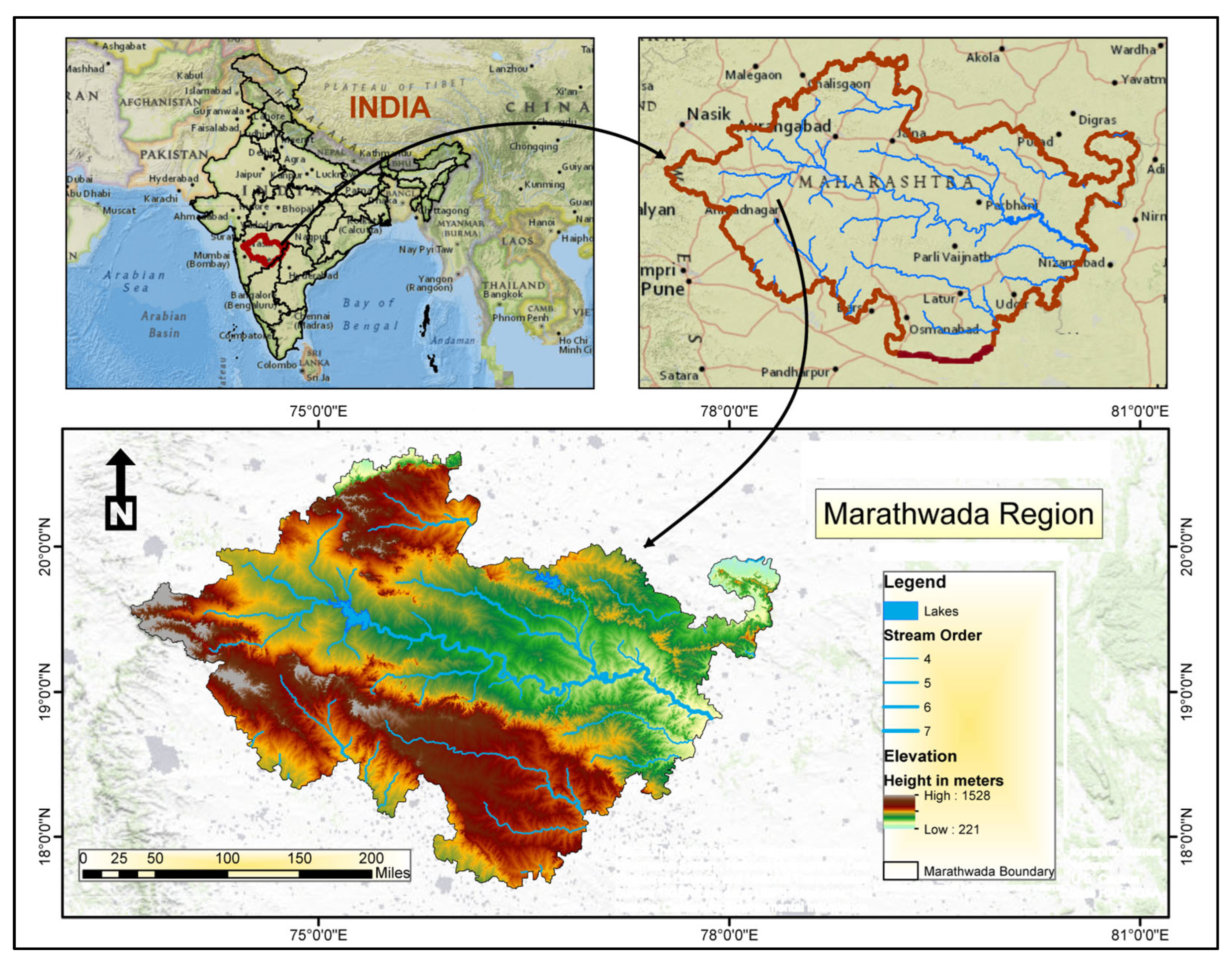
Disclaimer/Publisher’s Note: The statements, opinions and data contained in all publications are solely those of the individual author(s) and contributor(s) and not of MDPI and/or the editor(s). MDPI and/or the editor(s) disclaim responsibility for any injury to people or property resulting from any ideas, methods, instructions or products referred to in the content. |
© 2025 by the authors. Licensee MDPI, Basel, Switzerland. This article is an open access article distributed under the terms and conditions of the Creative Commons Attribution (CC BY) license (https://creativecommons.org/licenses/by/4.0/).