Article

Long-Term Retrospective Predicted Concentration of PM2.5 in Upper Northern Thailand Using Machine Learning Models

by
Sawaeng Kawichai
1,†,
Patumrat Sripan
1,†,
Amaraporn Rerkasem
1,
Kittipan Rerkasem
1,2,* and
Worawut Srisukkham
3,*
1
Research Institute for Health Sciences, Chiang Mai University, Chiang Mai 50200, Thailand
2
Clinical Surgical Research Center, Department of Surgery, Faculty of Medicine, Chiang Mai University, Chiang Mai 50200, Thailand
3
Department of Computer Science, Faculty of Science, Chiang Mai University, 239 Huay-Kaew Road, Suthep, Muang, Chiang Mai 50200, Thailand
*
Authors to whom correspondence should be addressed.
These authors contributed equally to this work.
Toxics 2025, 13(3), 170; https://doi.org/10.3390/toxics13030170
Submission received: 20 January 2025 / Revised: 21 February 2025 / Accepted: 24 February 2025 / Published: 27 February 2025
(This article belongs to the Special Issue Environmental Transport and Transformation of Pollutants)

Abstract

This study aims to build, for the first time, a model that uses a machine learning (ML) approach to predict long-term retrospective PM2.5 concentrations in upper northern Thailand, a region impacted by biomass burning and transboundary pollution. The dataset includes PM10 levels, fire hotspots, and critical meteorological data from 1 January 2011 to 31 December 2020. ML techniques, namely multi-layer perceptron neural network (MLP), support vector machine (SVM), multiple linear regression (MLR), decision tree (DT), and random forests (RF), were used to construct the prediction models. The best ML prediction model was selected considering root mean square error (RMSE), mean prediction error (MPE), relative prediction error (RPE) (the lower, the better), and coefficient of determination (R2) (the bigger, the better). Our study found that the ML model-based RF technique using PM10, CO2, O3, fire hotspots, air pressure, rainfall, relative humidity, temperature, wind direction, and wind speed performs the best when predicting the concentration of PM2.5 with an RMSE of 6.82 µg/m3, MPE of 4.33 µg/m3, RPE of 22.50%, and R2 of 0.93. The RF prediction model of PM2.5 used in this research could support further studies of the long-term effects of PM2.5 concentration on human health and related issues.

1. Introduction

Air pollution has been an issue in upper northern Thailand for several years, and the haze situation that has been caused by forest fires is a significant factor in this problem [1,2,3,4]. This burning causes a pollution problem throughout the dry season, which typically lasts from the end of February to the middle of April [1,2,3,4]. It is likely that exposure to specific environmental pollutants could have long-term effects and risk factors that contribute to an increased probability of sustaining lung cancer [5]. During this period, the amount of particulate matter smaller than 10 and 2.5 microns (PM10 and PM2.5) in the atmosphere exceeds the standards of Thailand. Moreover, the PM2.5 concentrations measured during the sampling period of 24 h exceeded the PM2.5 Thailand Ambient Air Quality Standard (50 µg/m3) by less than 30.60% (112 days in 2019) [6].
In this region, there is a significant gap in research on the long-term health effects of PM2.5 exposure, primarily due to the lack of comprehensive, long-term retrospective data on PM2.5 concentrations. The absence of data complicates the understanding of the impact of long-term air pollution exposure on health, particularly on lung cancer, cardiovascular diseases (CVDs), and chronic obstructive pulmonary disease (COPD) [5]. The lack of comprehensive long-term datasets limits the development of reliable evidence-based public health policies. In Chiang Mai, upper northern Thailand, PM2.5 monitoring was started in 2011, while PM2.5 data later became available in Lampang in 2018 and in other provinces in 2019, including Chiang Rai, Lamphun, Phayao, Phrae, Nan, and Mae Hong Son, owing to the limitations of resources. The importance of this work extends beyond regional limits, as the modeling methodology may be modified for application in other areas facing comparable problems with air quality. The combination of multiple sources of data, such as air pollutant concentrations, fire hotspot information, and meteorological variables, provides a thorough methodology for fulfilling the essential requirement for historical PM2.5 data in environmental health research. In upper northern Thailand, PM10 has been widely monitored for more than 20 years [7]. Predicting the results of PM2.5 values using PM10 [8,9,10] and fire hotspot data [11,12] with critical meteorological data [13,14] allows the study of the long-term effects of past exposure to PM2.5 on various health problems.
In previous studies, predictive methods have used multivariate statistical analysis, but in the last two decades, artificial intelligence technology using machine learning (ML) has been applied to create a model for forecasting or predicting air quality with an ability to predict results that are better than operational air quality measurements [15,16]. As a result, a wide range of research studies have been conducted that have applied various machine learning techniques such as artificial neural networks (ANNs) and support vector machines. Random forests classification has also been used to create a model for air quality prediction [15,16]. Studies on the model for predicting PM2.5 and PM10 concentrations revealed that various machine learning algorithms, capable of managing intricate and non-linear relationships among air quality variables, can effectively predict the value of new, unseen data with remarkable efficiency and precision [15,16,17,18,19]. ANNs are techniques for machine learning that mimic the neural activity of the human brain, appearing like nodes arranged in one or more layers. The nodes communicate with each other and store information in the form of the weight of each line connecting the nodes. This technique can retain knowledge that it has acquired and has been used in many tasks, including pattern recognition, bioinformatics, prediction, and other applications in many fields [19]. MLP neural networks are also widely used in predictive modeling. ML models provide highly accurate prediction results for PM2.5 and PM10 dust content [15,17,18,19]. This is the first time a model has been built that uses an ML approach to predict long-term retrospective PM2.5 concentrations in upper northern Thailand, a region impacted by biomass burning and transboundary pollution. The modeling framework developed here could not only be applied to northern Thailand, but also adapted to other regions with similar air quality issues. Furthermore, the retrospective study of PM2.5 data usually encounters spatial and temporal limitations due to the absence of government-provided monitoring stations for PM2.5 measurement in upper northern Thailand over the past decade. Therefore, several critical factors warrant the development of an ML model to predict retrospective PM2.5. Additionally, this integrative strategy not only bridges gaps in direct monitoring, but also advances our understanding of how exposure to these environmental factors could have long-term effects and risk factors that cause health issues. The main objective of this study is to apply ML methods to create a model for predicting retrospective PM2.5 values using air pollutant concentrations, fire hotspot data, and meteorological data.

2. Materials and Methods

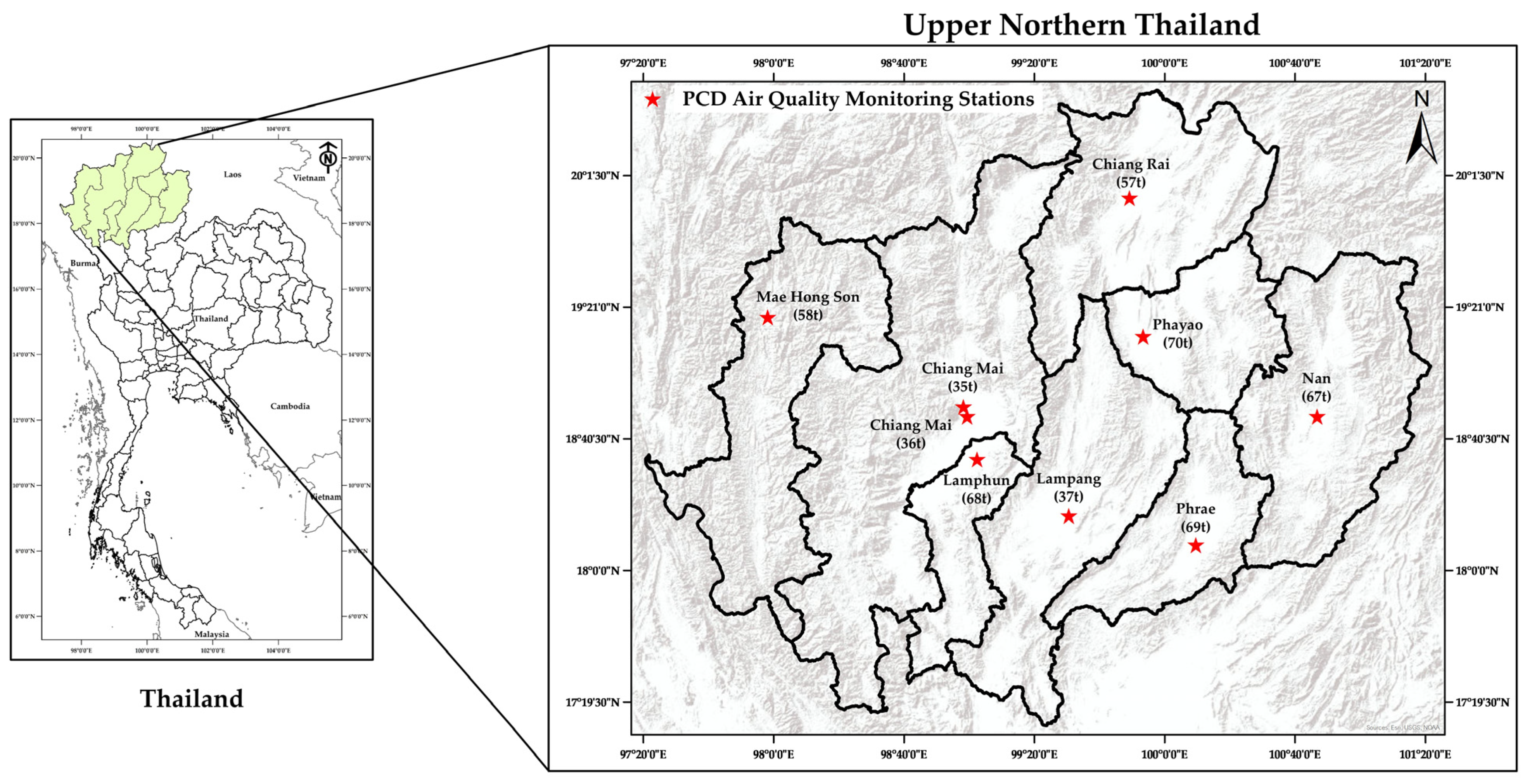
2.1. Descriptions of the Data

Air pollutant concentrations including PM2.5, PM10, CO2, SO2, NO2, and O3; fire hotspot data; and critical meteorological data including air pressure, rainfall, relative humidity, temperature, wind direction, and wind speed from 1 January 2011 to 31 December 2020 were collected from eight of the upper northern provinces of Thailand—Chiang Mai, Lampang, Chiang Rai, Lamphun, Phayao, Phrae, Nan, and Mae Hong Son—using the official database of the Pollution Control Department (PCD). In the PCD’s monitoring station, PM2.5 and PM10 concentrations were measured via the tapered element oscillating microbalance method (TEOM) and then averaged at the data center to produce a time series of the daily mean of air pollutant concentrations and meteorological data. Air quality and meteorological data were collected as daily mean values from fixed monitoring stations operated by the PCD in each province. All datasets were aggregated on a daily basis and assigned a location number, e.g., 35t and 36t represent Chiang Mai province. This synchronization ensured that the model used co-located information from all data sources for each day. The PCD’s monitoring stations, located in eight of the provinces of upper northern Thailand, are shown in Figure 1.
The daily fire hotspot number was retrieved from NASA’s Fire Information for Resource Management System (FIRMS). In this research, we obtained fire hotspot data from the MODIS Terra and Aqua Collection 6.1 via the NASA Level-1 and atmospheric archive and distribution system [20].

2.2. Predictive Model

The PM2.5 prediction models were constructed by employing twelve input parameters: (1) PM10, (2) CO2, (3) SO2, (4) NO2, (5) O3, (6) fire hotspots, (7) air pressure, (8) rainfall, (9) relative humidity, (10) temperature, (11) wind direction, and (12) wind speed. The PM2.5 data were collected during different time periods for each province—in 2011 for Chiang Mai, 2018 for Lampang, and 2019 for Chiang Rai, Lamphun, Phayao, Phrae, Nan, and Mae Hong Son. The SO2 data were not available for Mae Hong Son province, and the NO2 data in this province were incomplete and inconsistent. So, we built the predictive model of PM2.5 based on the data from Chiang Mai province, which has the oldest, longest, and most complete air quality and meteorological data from two monitoring stations (Figure 1).
Among 6974 records from Chiang Mai province used as training data, the amounts of missing data were 0.06% for NO2, 0.20% for SO2, 0.68% for rainfall, 1.15% for CO2, 1.15% for O3, and 47.57% for air pressure. We compared the performance of the model when using different numbers of features: (1) all 12 input features, (2) 11 input features (without SO2), and (3) 10 input features (without SO2 and NO2).
The predictive models were built using supervised ML. The models were trained on a labeled dataset, meaning that each input data point had a corresponding output, which was the PM2.5 concentration. The goal was for the model to learn the relationship between each input feature and the output so that it could predict the output for unseen data. One of the ML techniques used in this study was multi-layer perceptron (MLP), which is one of the most popular supervised neural network modelling techniques. It has been widely used in pattern recognition, bioinformatics, and computer vision and control systems [21]. MLP is a modern feed-forward neural network that consists of fully connected neurons or nodes. The nodes have a non-linear activation function, which is responsible for processing and giving answers to the next connecting nodes. It is usually trained using the backpropagation algorithm. Additionally, MLP consists of at least three layers of node networks: an input layer, a hidden layer, and an output layer [22]. In this study, we constructed MLP models using both a single hidden layer and two hidden layers. We employed the Levenberg–Marquardt backpropagation learning technique for both MLP models. We employed the Sigmoid activation function for the hidden layer and the Linear activation function for the output layer in a single hidden-layer configuration. The learning rate was 0.1, the momentum rate was 0.8, and the number of nodes varied from 1 to 50. Furthermore, for the MLP with two hidden layers, we employed the Sigmoid activation function for the hidden levels and the Linear activation function for the output layer. The learning rate was set at 0.1 and the momentum rate at 0.8, and the quantity of hidden-layer nodes varied from 1 to 30. We also used support vector machine (SVM), which is a kernel-based classification method. In general, it has to compute a linear function in a higher dimensional feature space, where the lower dimensional input data are mapped using a kernel function. It is used extensively in many fields such as prediction, pattern recognition, and classification [23]. This study involved constructing SVM models that utilize three distinct kernels: Linear, Polynomial, and Radial Basis functions. We employed grid search as the optimization method. The maximum objective evaluation and the maximum iteration were both set at 100. Multiple linear regression (MLR), which we also used, is a statistical model that estimates the relationships between one dependent variable and more independent variables by fitting multiple lines to the observed data. MLR extends a simple linear regression to include more than one explanatory variable to predict the outcome of a response variable [24,25]. Moreover, it is a widely used technique in many fields such as social sciences research, econometrics, and financial inference. In this study, we constructed the MLR model by using the “regress()” function for the multiple linear regression with a 95% confidence interval and setting epsilon (ε) to 0. Another technique we used was decision tree (DT), which is one of the general-purpose computationally intensive statistical algorithms for prediction and classification, artificial intelligence, machine learning, and knowledge discovery. DT has to do with using a procedure or rule repeatedly to generate subsetting of the target subject of data according to the values of associated input subjects to make partitions, and associated descendent leaves or nodes of the tree, that contain progressively similar intra-node target values and progressively dissimilar inter-node values at any given height of the tree [26]. This study involved the construction of a DT regression model utilizing a grid search optimizer, with the objective evaluation maximum set as 30. Random forests (RF) is another technique we used and is one of the famous ensemble machine learning techniques. Researchers have widely used it due to its good performance and simple usage [27,28]. This technique uses multiple decision trees. The trees’ predictors are taught using random sample data, and the distribution is the same for the predictors of all trees in the forest. The primary voting method is used to choose the greatest number of identical answers (majority voting). In this study, we developed an RF model with the following hyperparameters: the number of trees was set as 10, the maximum depth of the trees was set as 5, and the number of learning cycles for the trees was set as 200. The experiments in this work were performed using MATLAB R2018a. A summary of the hyperparameter settings for the machine learning models for the dataset from Chiang Mai province (air quality data, meteorological data, and fire hotspots) is shown in Table S1.

2.3. Model Validation

The best ML prediction model was selected considering the root mean square error (RMSE), mean prediction error (MPE), relative prediction error (RPE) (the lower, the better), and coefficient of determination (R2) (the bigger, the better) [29,30,31]. Additionally, in the evaluation of each run, 10-fold cross-validation [32] was implemented, dividing the dataset into 10 equally sized folds. In each iteration, 1 fold was designated as the validation set, with the remaining 9 folds used for training. This procedure was repeated until every fold had been used as the validation set once. This validation was applied to the dataset, which was divided into 70% for training and 30% for testing.

2.4. Prediction Evaluation Visual Check

The predicted PM2.5 was compared with the observed data to evaluate the performance of the model. Visual inspection was used to confirm that the predicted and observed data were aligned as their two-way plots were on the identical line. The RMSE, R2, MPE, and RPE were provided in addition to the graphical check. We performed the evaluation for both seen data (data for training model) and unseen data (data for testing model). This research used data from Chiang Mai province, which has the oldest, longest, and most complete data, for the visual check of the training data. Additionally, data from eight provinces were employed for the visual check of the unseen data.

3. Results

The air quality data, meteorological data, and data on fire hotspots in Chiang Mai province were separated into two parts, a dataset for training and a dataset for testing. The performances of the ML models—MLP, SVM, MLR, DT, and RF—are shown in Table 1.
When using all features, the RF model is the best model, considering its lowest RMSE at 6.7615 µg/m3, MPE at 4.1954 µg/m3, RPE at 22.29%, and highest R2 at 0.9318. Therefore, the RF model was selected and used for the next steps of this study.

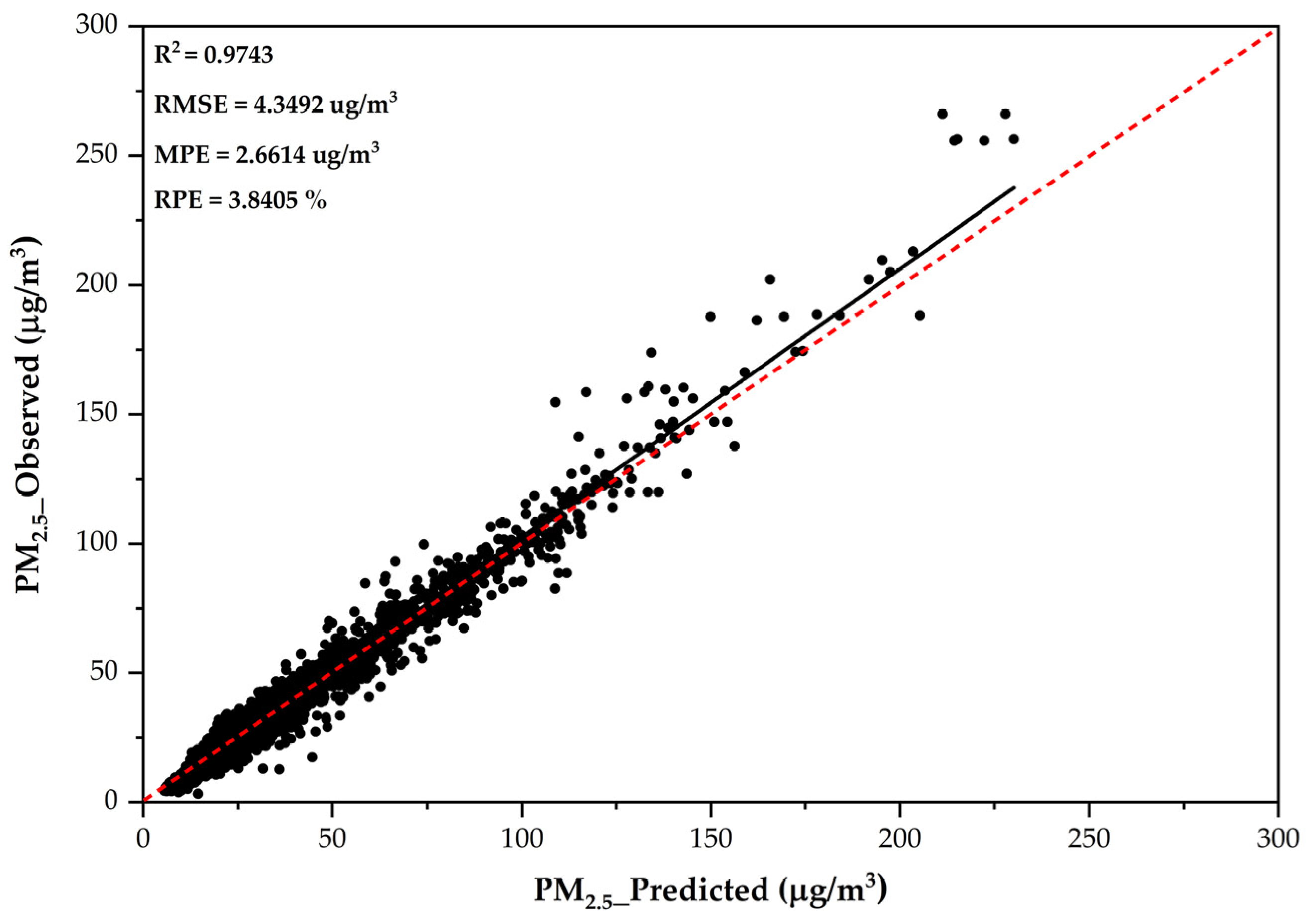
3.1. Performance of RF Model with Different Features

Based on the dataset from Chiang Mai province, after removing SO2, the RMSE, MPE, and RPE slightly increased to 6.8234 µg/m3, 4.2499 µg/m3, and 22.49%, respectively, and R2 was reduced to 0.9306. The performance of the model without SO2 was not different when compared to the full features model (p > 0.05). When NO2 was removed from the reduced model, the RMSE, MPE, and RPE increased to 6.8242 µg/m3, 4.3296 µg/m3, and 22.50%, respectively, while the R2 did not change. No significant change in model performance was observed when the number of features was reduced to 10. The performance of the model without SO2 and NO2 was not different when compared to the full model (p > 0.05) (Table 2).

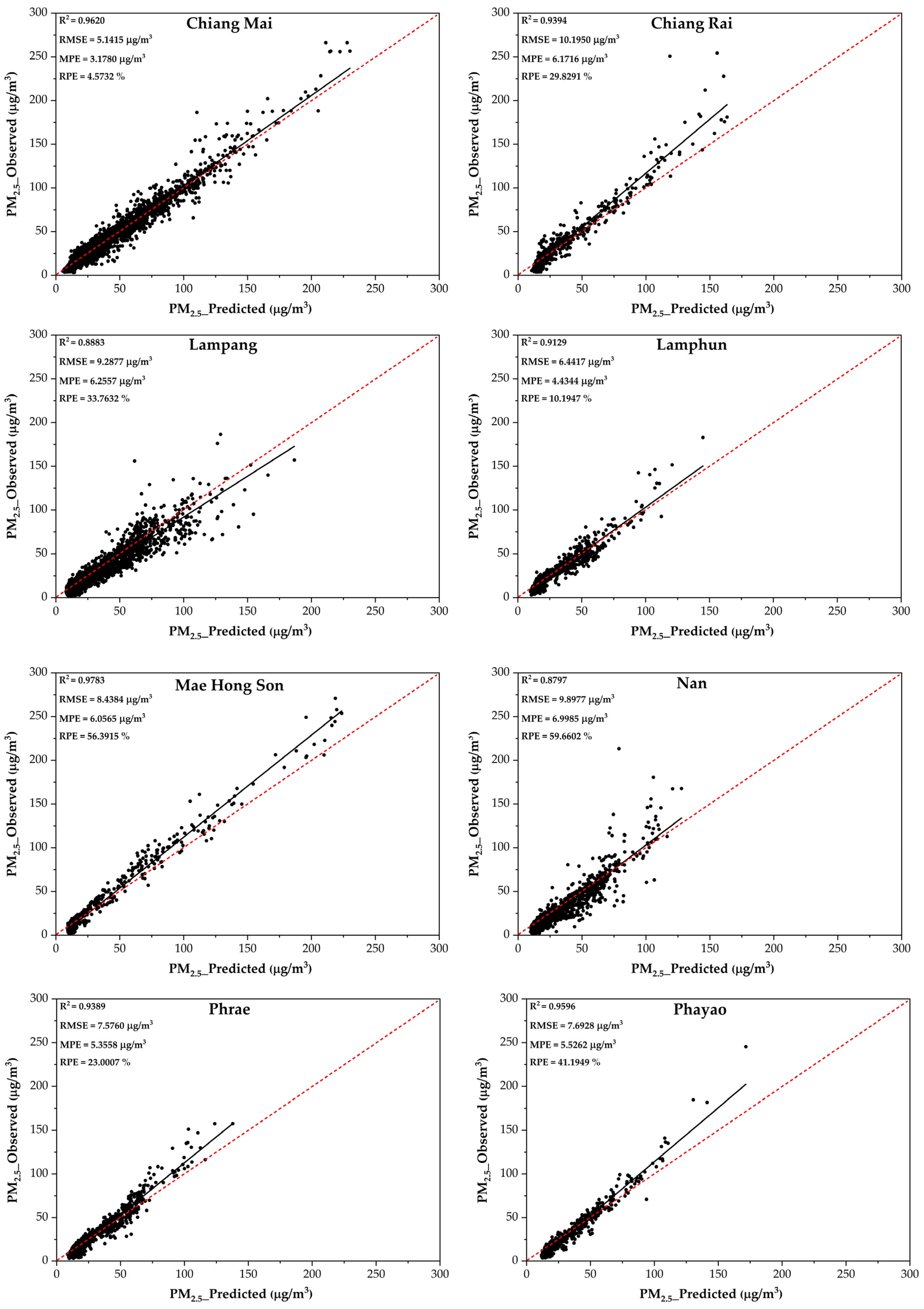
3.2. Performance of RF During PM2.5 Prediction in Eight Provinces in Upper Northern Thailand

The predictive model without SO2 and NO2 was used to predict PM2.5 in eight provinces in Northern Thailand. Figure 2 demonstrates the performance of the RF model on the training data, employing data from Chiang Mai province.
The value of R2 for the model used is 0.9743, while the R2 ranged from 0.8797 to 0.9783 for the testing data (Figure 3). The R2 was highest in Mae Hong Son province and lowest in Nan province. The performance of the model considering RMSE, MPE, and RPE indicated the same direction.

4. Discussion

From this study, it was found that the RF model was the most effective and had the highest accuracy in predicting PM2.5 concentrations compared to the other models. This is consistent with a study by Chen [33] that predicted PM2.5 using eight types of air quality data, as well as five types of meteorological data. Chen’s study found that using the RF model was the most efficient way to predict PM2.5, which had a relatively high R2 value of 0.94. In 2023, Vignesh et al. performed a study that employed ML techniques. There were nine models, and a tool was established to evaluate their performance and accuracy when predicting PM2.5 concentrations. The research, which was conducted in the United States, employed air pollution data collected over a period of five years, from 2017 to 2021 [34]. The investigation revealed that the RF model demonstrated high effectiveness when predicting concentrations of PM2.5, with an R2 of 0.77.
The higher concentrations of particulate pollution observed during the dry season are most likely a result of significant biomass burning, specifically from agricultural activities performed in preparation for the next agricultural season. Another issue is the transboundary transport of air pollution originating from neighboring countries such as Laos, Vietnam, and Myanmar, which is influenced by meteorological situations. These elements increase the problem of air quality in upper northern Thailand [35,36]. This study built a prediction model with data from Chiang Mai province. The unique model can be applied to eight provinces because of their comparable area characteristics. The primary factors contributing to air pollution in northern Thailand include biomass combustion, meteorological conditions, and geographical characteristics [37]. Moreover, a wide range of parameters have a significant impact on R2, with geographical data being particularly important. Various variables influence the value of R2, with Mae Hong Son province having the most significant influence. Mae Hong Son is a small province surrounded by forest. Mae Hong Son is located close to the Thailand–Myanmar border. Mae Hong Son province experiences multiple sources of air pollution, including transboundary effects, forest fires, and biomass burning, as indicated in prior research conducted by Kliengchuay et al. [38]. Forest fires play an important part in the emission of PM2.5 in this area. The complicated relationships between meteorological conditions and PM2.5 levels affect the numerous relations between PM2.5 and meteorology [39], while the lower R2 in an area like Nan, which is a large province, may be influenced by various meteorological parameters such as rainfall, wind direction, wind speed, temperature, relative humidity, and air pressure. Moreover, the lack of clarity regarding development across large areas could be contributing to the lower R2 [40,41].
Additionally, this study shows that the RF model is the most effective in predicting PM2.5, consistent with the findings of research conducted by Chen et al. [33] and Vignesh et al. [34]. However, our study differs from those studies in that we have included fire hotspots as a feature in our ML model for PM2.5 prediction, in addition to factors such as the environment, the climate, and geographical characteristics. The topography, meteorological data, and agriculture of Southeast Asia significantly contributes to the prevalence of monoculture farming, resulting in an important number of fire hotspots. These regions in Southeast Asia show evidence of biomass burning, which emits PM2.5 pollutants [1,2,3,4]. Thus, our study employs the number of fire hotspots as one of the important features for modeling the PM2.5 predictor.
The retrospective PM2.5 data from our research could be helpful for studying the long-term effects of PM2.5 concentrations on human health issues such as lung cancer, cardiovascular diseases (CVDs), and chronic obstructive pulmonary disease (COPD). There are relatively few studies on the impact of exposure to PM2.5 on lung cancer incidence rates among Asian populations. There are literature review studies that aim to explore the relationship between PM2.5 and lung cancer incidence and mortality. One review study shows that some studies have found a significant relationship between PM2.5 and the incidence of lung cancer, but other studies did not find this relationship [5]. The limited number of studies on the impact of exposure to PM2.5 on lung cancer may be caused by the limited long-term PM2.5 data, particularly in low- and middle-income countries. Our predicted PM2.5 data, as shown in Supplementary Table S2, could be included in epidemiological health outcome prediction models to clarify PM2.5-related health risks in upper northern Thailand. Additionally, investigating the relationships between socio-economic characteristics, healthcare accessibility, and health outcomes associated with PM2.5 would enhance comprehension of the differences in disease burden. Long-term cohort studies that monitor individuals over time, considering both environmental exposures and personal health data, could be essential for enhancing exposure response models and guiding public health strategies to reduce the harmful effects of air pollution. Finally, the PM2.5 concentration values from the past 10 years (2011 to 2020) that were predicted during our study could be used to investigate the long-term impact of PM2.5 on acute and chronic respiratory diseases, as well as to study other health-related effects of PM2.5 in eight provinces in the upper northern region of Thailand, an area where PM2.5 concentration levels are reported to exceed Thailand’s ambient air quality standard every year.

5. Conclusions

This study found that the RF model was the most effective in predicting PM2.5 concentrations, outperforming other models in terms of accuracy. It also highlights the significant impact of biomass burning and fire hotspots on the prediction of PM2.5 concentrations. Our study illustrates the significance of employing numerous data sources and effective methods for modeling in environmental studies. Moreover, future work could apply the RF model, which is a highly effective tool for predicting long-term PM2.5 concentrations (RMSE of 6.82 μg/m3, MPE of 4.33 μg/m3, RPE of 22.50%, and R2 of 0.93), to other regions or countries with similar environmental conditions, including biomass burning and transboundary pollution. The predicted PM2.5 concentrations could lead to improved air quality management strategies and more informed public health policies. Furthermore, our research suggests that the prediction model of prolonged PM2.5 concentrations could offer a foundation for further epidemiological studies on the long-term effects of PM2.5 concentrations on human health and related problems.

Supplementary Materials

The following supporting information can be downloaded at: https://www.mdpi.com/article/10.3390/toxics13030170/s1, Table S1: The hyperparameters of the machine learning models for the dataset from Chiang Mai province (air quality data, meteorological data, and fire hotspots); Table S2: The predicted PM2.5 concentrations in 8 provinces in northern Thailand, 2011–2020.

Author Contributions

Conceptualization, S.K., P.S., K.R. and W.S.; data curation, S.K., P.S. and W.S.; formal analysis, P.S. and W.S.; funding acquisition, K.R. and W.S.; investigation, A.R.; methodology, P.S. and W.S.; supervision, K.R. and W.S.; validation, P.S.; writing—original draft, S.K., P.S., A.R., K.R. and W.S.; writing—review and editing, S.K., P.S., A.R., K.R. and W.S. All authors will be updated at each stage of manuscript processing, including submission, revision, and revision reminder, via emails from our system or the assigned Assistant Editor. All authors have read and agreed to the published version of the manuscript.

Funding

This research was supported by the Coordinating Center for Thai Government Science and Technology Scholarship Students (CSTS) and the National Science and Technology Development Agency (NSTDA). It was partially supported by fundamental fund 2567 (FF67) from Chiang Mai University, and the PM2.5 project was supported by Chiang Mai University.

Institutional Review Board Statement

Not applicable.

Informed Consent Statement

Not applicable.

Data Availability Statement

The datasets used and/or analyzed during the current study are available from the corresponding author upon reasonable request.

Acknowledgments

The authors express their gratitude to the Coordinating Center for Thai Government Science and Technology Scholarship Students (CSTS); the National Science and Technology Development Agency (NSTDA) THAILAND; the Department of Computer Science, Faculty of Science, Chiang Mai University, Chiang Mai, Thailand; and the Research Institute for Health Sciences, Chiang Mai University, Chiang Mai, Thailand.

Conflicts of Interest

The authors declare that they have no competing interests.

Abbreviations

The following abbreviations are used in this manuscript:
ANNsArtificial neural networks
COPDChronic obstructive pulmonary disease
CVDsCardiovascular diseases
DTDecision tree
FIRMSFire Information for Resource Management System
MLMachine learning
MLPMulti-layer perceptron neural network
MLRMultiple linear regression
MODISModerate Resolution Imaging Spectroradiometer
NASANational Aeronautics and Space Administration
PCDPollution Control Department
PM2.5Particulate matter smaller than 2.5 microns
PM10Particulate matter smaller than 10 microns
RFRandom forests
SVMSupport vector machine
TEOMTapered element oscillating microbalance method

References

  1. Chansuebsri, S.; Kraisitnitikul, P.; Wiriya, W.; Chantara, S. Fresh and aged PM2.5 and their ion composition in rural and urban atmospheres of Northern Thailand in relation to source identification. Chemosphere 2021, 286, 131803. [Google Scholar] [CrossRef]
  2. Kawichai, S.; Prapamontol, T.; Cao, F.; Song, W.; Zhang, Y. Source Identification of PM2.5 during a smoke haze period in Chiang Mai, Thailand, using stable carbon and nitrogen isotopes. Atmosphere 2022, 13, 1149. [Google Scholar] [CrossRef]
  3. Kawichai, S.; Prapamontol, T.; Cao, F.; Song, W.; Zhang, Y.L. Characteristics of carbonaceous species of PM2.5 in Chiang Mai city, Thailand. Aerosol Air Qual. Res. 2024, 24, 230269. [Google Scholar] [CrossRef]
  4. Song, W.; Hong, Y.; Zhang, Y.; Cao, F.; Rauber, M.; Santijitpakdee, T.; Kawichai, S.; Prapamontol, T.; Szidat, S.; Zhang, Y.L. Biomass burning greatly enhances the concentration of fine carbonaceous aerosols at an urban area in upper northern Thailand: Evidence from the radiocarbon-based source apportionment on size-resolved aerosols. J. Geophys. Res. Atmos. 2024, 129, e2023JD040692. [Google Scholar] [CrossRef]
  5. Huang, F.; Pan, B.; Wu, J.; Chen, E.; Chen, L. Relationship between exposure to PM2.5 and lung cancer incidence and mortality: A meta-analysis. Oncotarget 2017, 8, 43322–43331. [Google Scholar] [CrossRef]
  6. Department of Pollution Control. Manual Report: Air Quality Data Monitoring; Pollution Control Department: Bangkok, Thailand, 2024; Available online: https://www.pcd.go.th/wp-content/uploads/2021/03/pcdnew-2021-04-07_06-54-58_342183.pdf (accessed on 10 January 2025).
  7. Pollution Control Department. Air Quality and Noise. Available online: http://air4thai.pcd.go.th/webV3/#/Home (accessed on 10 January 2025).
  8. Sirignano, C.; Riccio, A.; Chianese, E.; Ni, H.; Zenker, K.; D’Onofrio, A.; Meijer, H.A.J.; Dusek, U. High contribution of biomass combustion to PM2.5 in the city centre of Naples (Italy). Atmosphere 2019, 10, 451. [Google Scholar] [CrossRef]
  9. Xu, G.; Jiao, L.; Zhao, S.; Cheng, J. Spatial and temporal variability of PM2.5 concentration in China. Wuhan Univ. J. Nat. Sci. 2016, 21, 358–368. [Google Scholar] [CrossRef]
  10. Zhuang, Y.; Chen, D.; Li, R.; Chen, Z.; Cai, J.; He, B.; Gao, B.; Cheng, N.; Huang, Y. Understanding the influence of crop residue burning on PM2.5 and PM10 concentrations in China from 2013 to 2017 using MODIS data. Int. J. Environ. Res. Public Health 2018, 15, 1504. [Google Scholar] [CrossRef]
  11. Geng, G.; Murray, N.L.; Tong, D.; Fu, J.S.; Hu, X.; Lee, P.; Meng, X.; Chang, H.H.; Liu, Y. Satellite-based daily PM2.5 estimates during fire seasons in Colorado. J. Geophys. Res. Atmos. 2018, 123, 8159–8171. [Google Scholar] [CrossRef]
  12. Lee, H.H.; Iraqui, O.; Gu, Y.; Yim, S.H.L.; Chulakadabba, A.; Tonks, A.Y.M.; Yang, Z.; Wang, C. Impacts of air pollutants from fire and non-fire emissions on the regional air quality in southeast asia. Atmos. Chem. Phys. 2018, 18, 6141–6156. [Google Scholar] [CrossRef]
  13. Chen, Z.; Chen, D.; Zhao, C.; Kwan, M.P.; Cai, J.; Zhuang, Y.; Zhao, B.; Wang, X.; Chen, B.; Yang, J.; et al. Influence of meteorological conditions on PM2.5 concentrations across China: A review of methodology and mechanism. Environ. Int. 2020, 139, 105558. [Google Scholar] [CrossRef]
  14. Li, Y.; Chen, Q.; Zhao, H.; Wang, L.; Tao, R. Variations in PM10, PM2.5 and PM1.0 in an urban area of the Sichuan basin and their relation to meteorological factors. Atmosphere 2015, 6, 150–163. [Google Scholar] [CrossRef]
  15. Suleiman, A.; Tight, M.R.; Quinn, A.D. Applying machine learning methods in managing urban concentrations of traffic-related particulate matter (PM10 and PM2.5). Atmos. Pollut. Res. 2019, 10, 134–144. [Google Scholar] [CrossRef]
  16. Zhang, G.; Rui, X.; Fan, Y. Critical review of methods to estimate PM2.5 concentrations within specified research region. ISPRS Int. J. Geo-Inf. 2018, 7, 368. [Google Scholar] [CrossRef]
  17. Biancofiore, F.; Busilacchio, M.; Verdecchia, M.; Tomassetti, B.; Aruffo, E.; Bianco, S.; Di Tommaso, S.; Colangeli, C.; Rosatelli, G.; Di Carlo, P. Recursive neural network model for analysis and forecast of PM10 and PM2.5. Atmos. Pollut. Res. 2017, 8, 652–659. [Google Scholar] [CrossRef]
  18. Chen, M.J.; Yang, P.H.; Hsieh, M.T.; Yeh, C.H.; Huang, C.H.; Yang, C.M.; Lin, G.M. Machine learning to relate PM2.5 and PM10 concentrations to outpatient visits for upper respiratory tract infections in Taiwan: A nationwide analysis. World J. Clin. Cases. 2018, 6, 200–206. [Google Scholar] [CrossRef]
  19. Gholizadeh, A.; Neshat, A.A.; Conti, G.O.; Ghaffari, H.R.; Aval, H.E.; Almodarresi, S.A.; Aval, M.Y.; Zuccarello, P.; Taghavi, M.; Mohammadi, A.; et al. PM2.5 concentration modeling and mapping in the urban areas. Model. Earth Syst. Environ. 2019, 5, 897–906. [Google Scholar] [CrossRef]
  20. Fire Information for Resource Management System. Available online: https://firms.modaps.eosdis.nasa.gov/active_fire (accessed on 24 October 2024).
  21. Hagan, M.; Demuth, H.; Beale, M. Neural Network Design; PWS Publishing: Boston, MA, USA, 1997. [Google Scholar]
  22. Cybenko, G. Approximation by superpositions of a sigmoidal function. Math. Cont. Sig. Syst. 1989, 2, 303–314. [Google Scholar] [CrossRef]
  23. Basak, D.; Pal, S.; Patranabis, D. Support vector regression. Neural Inf. Process. -Lett. Rev. 2007, 11, 203–224. [Google Scholar]
  24. Freedman, D. Statistical Models: Theory and Practice; Cambridge University Press: Cambridge, UK, 2005. [Google Scholar]
  25. Tranmer, M.; Murphy, J.; Elliot, M.; Pampaka, M. Multiple Linear Regression, 2nd ed.; Cathie Marsh Institute Working Paper 2020–01; Cathie Marsh Institute for Social Research: Manchester, UK, 2020; Available online: https://hummedia.manchester.ac.uk/institutes/cmist/archive-publications/working-papers/2020/multiple-linear-regression.pdf (accessed on 10 January 2025).
  26. de Ville, B. Decision trees. WIREs Comp Stats. 2013, 5, 448–455. [Google Scholar] [CrossRef]
  27. Breiman, L. Random Forests. Mach. Learn. 2001, 45, 5–32. [Google Scholar] [CrossRef]
  28. González, S.; García, S.; Del Ser, J.; Rokach, L.; Herrera, F. A practical tutorial on bagging and boosting based ensembles for machine learning: Algorithms, software tools, performance study, practical perspectives and opportunities. Inf. Fusion 2020, 64, 205–237. [Google Scholar] [CrossRef]
  29. Sun, Y.; Zeng, Q.; Geng, B.; Lin, X.; Sude, B.; Chen, L. Deep learning architecture for estimating hourly ground-level PM2.5 using satellite remote sensing. IEEE Geosci. Remote Sens. Lett. 2019, 16, 1343–1347. [Google Scholar] [CrossRef]
  30. Wang, W.; Zhao, S.; Jiao, L.; Taylor, M.; Zhang, B.; Xu, G.; Hou, H. Estimation of PM2.5 concentrations in China using a spatial back propagation neural network. Sci. Rep. 2019, 9, 13788. [Google Scholar] [CrossRef]
  31. Yun, E.; Tornero-Velez, R.; Purucker, S.; Chang, D.; Edginton, A. Evaluation of quantitative structure property relationship algorithms for predicting plasma protein binding in humans. Comput. Toxicol. 2020, 17, 100142. [Google Scholar] [CrossRef] [PubMed]
  32. Jain, A.; Duin, R.; Mao, J. Statistical pattern recognition: A review. IEEE Trans. Pattern Anal. Mach. Intell. 2000, 22, 4–37. [Google Scholar] [CrossRef]
  33. Chen, M.; Chen, Y.C.; Chou, T.Y.; Ning, F.S. PM2.5 Concentration prediction model: A CNN-RF ensemble framework. Int. J. Environ. Res. Public Health 2023, 20, 4077. [Google Scholar] [CrossRef]
  34. Vignesh, P.P.; Jiang, J.H.; Kishore, P. Predicting PM2.5 concentrations across USA using machine learning. Earth Space Sci. 2023, 10, e2023EA002911. [Google Scholar] [CrossRef]
  35. Amnuaylojaroen, T.; Kreasuwun, J. Investigation of fine and coarse particulate matter from burning areas in Chiang Mai, Thailand using the WRF/CALPUFF. Chiang Mai J. Sci. 2011, 39, 311–326. [Google Scholar]
  36. Punsompong, P.; Pani, S.; Wang, S.H.; Thao, P. Assessment of biomass-burning types and transport over Thailand and the associated health risks. Atmos. Environ. 2020, 247, 118176. [Google Scholar] [CrossRef]
  37. Suriyawong, P.; Chuetor, S.; Samae, H.; Piriyakarnsakul, S.; Amin, M.; Furuuchi, M.; Hata, M.; Inerb, M.; Phairuang, W. Airborne particulate matter from biomass burning in Thailand: Recent issues, challenges, and options. Heliyon 2023, 9, e14261. [Google Scholar] [CrossRef] [PubMed]
  38. Kliengchuay, W.; Meeyai, A.; Worakhunpiset, S.; Tantrakarnapa, K. Relationships between meteorological parameters and particulate matter in Mae Hong Son Province, Thailand. Int. J. Environ. Res. Public Health 2018, 15, 2801. [Google Scholar] [CrossRef] [PubMed]
  39. Chen, Z.; Xie, X.; Cai, J.; Danlu, C.; Gao, B.; He, B.; Cheng, N.; Xu, B. Understanding meteorological influences on PM2.5 concentrations across China: A temporal and spatial perspective. Atmos. Chem. Phys. 2018, 18, 5343–5358. [Google Scholar] [CrossRef]
  40. Chang, C.H.; Hsiao, Y.L.; Hwang, C. Evaluating spatial and temporal variations of aerosol optical depth and biomass burning over southeast asia based on satellite data products. Aerosol Air Qual. Res. 2015, 15, 2625–2640. [Google Scholar] [CrossRef]
  41. Mohammadi, F.; Teiri, H.; Hajizadeh, Y.; Abdolahnejad, A.; Ebrahimi, A. Prediction of atmospheric PM2.5 level by machine learning techniques in Isfahan, Iran. Sci. Rep. 2024, 14, 2109. [Google Scholar] [CrossRef] [PubMed]
Figure 1. The Pollution Control Department (PCD)’s monitoring stations in upper northern Thailand.
Toxics 13 00170 g001
Figure 2. The performance of the RF model during PM2.5 prediction using training data from Chiang Mai province.
Toxics 13 00170 g002
Figure 3. The performance of the RF model during PM2.5 prediction using testing data from eight provinces in upper northern Thailand.
Toxics 13 00170 g003
Table 1. Performances of ML models for PM2.5 prediction using different numbers of features.
MethodsPrediction Performances
10 Features (Without SO2 and NO2)11 Features (Without SO2)12 Features
RMSER2MPERPERMSER2MPERPERMSER2MPERPE
MLP (1 Hidden Layer)7.22870.92114.794423.887.21360.92144.884523.847.18020.92214.812123.73
MLP (2 Hidden Layers)7.33280.91814.818424.247.32650.91894.882224.197.23670.92104.885423.91
SVM (Linear Kernel)10.74020.82238.205735.5111.16080.81118.479136.7911.76840.77529.253038.99
SVM (Polynomial Kernel)12.94200.736710.239142.7012.52870.76029.817441.3812.16420.76218.982640.08
SVM (RBF Kernel)12.07700.77488.926139.9112.68470.75399.600741.8212.12470.77559.006740.01
MLR7.74230.91035.222325.557.74150.91035.227025.557.70560.91115.214125.44
DT9.07470.87625.822429.968.78430.88405.598929.018.93780.88005.614129.52
RF6.82420.93064.329622.506.82340.93064.249922.496.76150.93184.195422.29
Note: RMSE: root mean square error (µg/m3); R2: coefficient of determination; MPE: mean prediction error (µg/m3); RPE: relative prediction error (%).
Table 2. Comparison between PM2.5 prediction performances of RF model with different features.
Performances12 Features11 Featuresp-Value10 Featuresp-Value
Average RMSE6.78596.81100.87986.82160.9397
Average R20.93130.93080.93970.93070.8798
Average MPE4.32904.25330.25684.19440.3258
Average RPE22.374022.45510.939722.48841.0000
Disclaimer/Publisher’s Note: The statements, opinions and data contained in all publications are solely those of the individual author(s) and contributor(s) and not of MDPI and/or the editor(s). MDPI and/or the editor(s) disclaim responsibility for any injury to people or property resulting from any ideas, methods, instructions or products referred to in the content.

