Optimizing Resilient Sustainable Citrus Supply Chain Design

Abstract

Background: Growing environmental concerns and the vulnerability of global supply chains to disruptions, such as pandemics, natural disasters, and logistical failures, necessitate the design of sustainable and resilient supply chains. Methods: A novel multi-period mixed-integer linear programming model is developed with the objective of maximizing supply chain profit to design a complete citrus supply chain, which incorporates the production of citrus fruit and juice, and accommodates resilience and sustainability perspectives. Results: A comprehensive citrus supply chain scenario is presented to support the applicability of the proposed model, leveraging real data from citrus supply chain stakeholders in Egypt. Moreover, an actual case study involving a citrus processing company in Egypt is demonstrated. Gurobi software is used to solve the developed model. To build a resilient supply chain which can cope with different disruptions, different scenarios are modeled and strategies for having multiple suppliers, backup capacity, and alternative logistics routes are evaluated. Conclusions: The findings underscore the critical role of resilience in supply chain management, particularly in the agri-food sector. Moreover, the proposed model not only maximizes supply chain profitability but also equips stakeholders with the tools necessary to navigate challenges effectively.

1. Introduction

In today’s interconnected global economy, supply chains have become increasingly complex due to strategies like global outsourcing, international manufacturing, and just-in-time deliveries. Although these strategies are beneficial, supply chains became more vulnerable to issues such as variable exchange rates and political and economic instability. Recent events such as the COVID-19 pandemic have caused significant disruptions, highlighting the need for enhanced resilience. The pandemic alone adversely affected over 94% of the top 1000 companies [1], emphasizing the importance of resilient supply chain management. Unlike traditional risk management, which deals with identifying, assessing, and mitigating risks, supply chain resilience (SCR) addresses coping with major disruptions that threaten supply chain continuity. Emenike & Falcone [2] defined SCR as the ability to withstand stress or system failures and minimize disruption impacts. Achieving SCR involves studying various strategies and balancing the costs with product availability to effectively mitigate disruptions. Given that environmental resources are the most precious and finite resource available to humans, the sustainability of supply chains has recently drawn the attention of businesses, governments, researchers, and consumers.

The agriculture industry is a significant contributor to the global economy, specifically in developing countries. Agri-food supply chains (ASCs) account for about 20% of a developing country’s Gross Domestic Product (GDP) [3]. Resilience in ASCs has become crucial due to increasing volatility, driven by climate variability, resource inadequacies, and disruptions. This volatility impacts supply and demand, stressing the need for resilient strategies. Sustainability is also essential in ASCs to cope with challenges such as population growth, climate change, and food waste.

Citrus is a globally significant fruit, with a global production of around 169 million tons in 2023 [4]. The global trade value of citrus in 2023 was around 25 million tons [5]. The Middle East is a vital region in the global citrus market [6], specifically Egypt, which plays a crucial role in the global agricultural landscape. Egypt’s production of oranges in 2024 was 3.7 million tons [7]. According to the USDA/FAS report of 2021, Egypt holds the third position worldwide in terms of agricultural production and export volumes [8]. Egypt exported 1.5 million tons of citrus products in 2023 [5]. This emphasizes the importance of the citrus supply chain in Egypt, motivating the focus of this research. In recent years, the growing environmental concerns and increasing demand for sustainable practices have prompted the re-evaluation of the entire citrus supply chain. As Egypt is heavily reliant on agricultural exports, studying and mitigating ASC disruptions is vital for the continuity of these supply chains under different circumstances, since they stretch across international regions making them more vulnerable. These aspects reflect the necessity of having a resilient and sustainable citrus supply chain network.

In their study, Beshara et al. [9] have revealed that there is a significant gap in studying ASCs for a specific food type. Moreover, there are calls for modeling and quantifying resilience-mitigating strategies to achieve supply chain resilience [8,10]. In addition, there is a lack of citrus processor echelon in the supply chain, even though this process adds value to citrus fruit [6]. According to the existing literature, there is a gap in designing a complete citrus supply chain involving the production of citrus fruit and juice and dealing with citrus waste simultaneously. Therefore, the primary objective of this study is to design a completely resilient and sustainable citrus supply chain network. This network helps in mitigating the impact of disruptions while upholding the supply chain’s performance through adopting one of the resilience strategies, while sustainability is realized through supply chain profit maximization, waste reduction, and generated processing waste valorization by selling it to intermediaries or processors working with this waste. In other words, this study answers the following questions: (1) What is the optimum citrus supply chain network design that maximizes the supply chain profit, in terms of determining the operational status of each facility, quantities transported between all echelons, processing quantities at packhouses and processors, and inventory levels at each facility? (2) What is the recommended resilient strategy to be applied in the supply chain network in case of disruptions at suppliers, packhouses, processors, and outbound logistics?

The main contribution of this study is twofold. First, a multi-period mixed-integer linear programming model is formulated to design a complete resilient sustainable citrus supply chain network, encompassing the entire supply chain from farm to fork that includes citrus fruit, juice, and waste. Secondly, the study addresses the most common scenarios of disruption for this supply chain and provides evidence of the best strategies to withstand these disruptions.

This paper is organized as follows: A brief overview on resilience in ASCs and citrus supply chain studies is introduced in the following section. Section 3 presents the proposed mathematical model for designing a citrus supply chain (CSC) network with an objective of maximizing supply chain profits. A complete CSC scenario and an actual case study for a citrus processing company in Egypt are illustrated in Section 4. In this section, the disruption scenarios evaluated to determine the most appropriate resilience strategy for each type of disruption are demonstrated. Section 5 shows the models’ results and the results of different disruption scenarios. Finally, Section 6 presents the conclusions, managerial insights, and future work.

2. Literature Review

This section provides an overview of the most relevant research papers in two fields: (1) resilience in agri-food supply chains (ASCs) and (2) the modeling of citrus supply chains (CSCs).

2.1. Resilience in Agri-Food Supply Chains

Several strategies can be implemented to enhance supply chain resilience; these strategies can be categorized into proactive and reactive strategies. Proactive strategies include expanding manufacturing capacity, having capacity buffers, multiple sourcing, having contracts with backup suppliers, fortifying facilities, maintaining safety stock, and having several transport routes. These actions are preventive and ensure the flexibility and readiness of the supply chain before the occurrence of disruptions, while reactive strategies are activated in response to disruptions, focusing on the responsiveness of the supply chain. They involve using backup facilities, suppliers, and transport routes; expanding capacity; and selecting the best alternative scenario.

ASC resilience is crucial for maintaining a continuous safe flow of food products from farm to fork. In the context of ASCs, the primary disruptions are weather-related or politically driven, impacting supply, demand, and logistics [11]. Disruptions in ASCs can differ from both ends of the supply chain. Supply disruptions resulting from weather conditions could affect the timing, quality, and quantity of supply. In contrast, demand-related disruptions arise due to political and social issues such as a change in tariffs, variability in local market prices, and any shift in customer preferences. These disturbances may disrupt product flow and result in significant waste [12].

The implemented mitigation strategy depends on the type of disruption and the supply chain echelon affected.

Table 1. Type of disruption and the strategy used to mitigate its effect.

Reference	Type of Disruption		Strategy
	Complete	Partial	Proactive	Reactive
Behzadi et al. [12]		D		BT and BM
Esteso et al. [14]		DC–P	Tech and MS	BS and Cp
Stone & Rahimifard [15]	X		Tech, I, and MS	BS, BT, Cp, Cd, and A
Ravulakollu et al. [16]	X		Tech
Bottani et al. [17]		S–D	MS
Liao et al. [18]		D	I
G. Zhao et al. [11]	X		--	--
Behzadi et al. [19]		T		BT
Mohib & Deif [20]		S	MS
Sharma et al. [21]	X		Tech
Gholami-Zanjani, Jabalameli et al. [13]		D–P	Tech and MS	BS and Cp
Gholami-Zanjani, Klibi et al. [22]	X			BS, Cp, Cd, and A
Abu Hatab et al. [23]	X		--	--
Li et al. [10]		S–R	Tech and F	A
Ali et al. [24]	X		--	--
G. Zhao et al. [25]	X		MS and I	BS, BT, Cp, and Cd
Li & Zhang [26]	X		MS and I	A

S: Supplier, P: Producer, D: Demand, T: Transportation, DC: Distribution Center, R: Retailer, MS: Multiple Supplier, Tech: Technological Investment, I: Inventory Safety Stock, F: Fortification, BS: Backup Supplier, BT: Backup Transport, BM: Backup Market, Cp: Capacity Buffer at P, Cd: Capacity Buffer at DC, A: Alternative Scenarios.

outlines the different disruptions and corresponding mitigation strategies in the literature. Distributions are addressed at certain echelons (partially) or all over the supply chain. Proactive strategies are more frequently studied in the research, specifically multiple supplier and technological investment strategies. For example, Gholami-Zanjani, Jabalameli et al. [13] explored how investing in technological infrastructure can enhance collaboration across the supply chain and maintain profitability despite disruptions at the producer or distribution center. On the contrary, reactive strategies are less frequently studied, with most research focusing on backup suppliers or capacity buffers at the producer. The focus on backup suppliers is likely due to the significant vulnerability of agri-food suppliers to disruptions [12].

According to Table 1, multiple or backup facility strategies are not extensively studied in ASC research. This is likely because supply and demand are critical points in the supply chain, since farms are highly susceptible to changes and demand is highly dependable on customers’ preferences. Facilities like producers or distribution centers may be exposed to disruptions, causing a halt in the supply chain. So, having multiple or backup facilities may mitigate the effect of disruptions. Accordingly, there is a need to study the impact of having multiple facilities across the entire chain and backup facilities at the critical echelons.

2.2. Citrus Supply Chains

Different research topics are addressed in the papers modeling CSCs. The most prevalent topics are summarized in

Table 2. Research topics in CSC papers.

Reference	Export	Traceability	Facility Location	Quality	Waste	CO2 Emissions	Economic	Social	Contracts	CircularityConsideration	Standardization	Logistics	Technology	Pricing
Miranda-Ackerman et al. [27]			X			X	X		X	X			X
Cheraghalipour et al. [30]			X		X		X			X		X
Imbachi et al. [31]		X			X		X						X
Roghanian & Cheraghalipour [32]			X		X	X	X			X		X
Aslan et al. [33]	X		X	X	X		X		X
Liao et al. [18]			X			X	X					X
Sahebjamnia et al. [34]			X				X					X
Darley-waddilove [29]	X			X	X		X				X
Goodarzian & Fakhrzad [35]					X		X					X		X
Peña Orozco et al. [36]					X		X
Güner & Utku [37]				X	X		X
Alzubi & Noche [38]			X		X	X						X
Alzubi et al. [39]					X	X	X			X		X
Goodarzian et al. [40]			X		X	X	X	X		X
Peña-Orozco et al. [28]					X	X	X	X
Paredes-Rodríguez et al. [41]			X			X	X	X				X
Goodarzian et al. [42]						X	X

. The economic and environmental sustainability pillars are the most addressed topics, while the social aspect is discussed only twice. Economic sustainability is the primary focus, followed by environmental concerns such as waste and CO₂ emissions, which are often addressed together. For example, Miranda-Ackerman et al. [27] proposed a mathematical model that identified the optimal supply chain configuration considering operational, financial, and environmental factors, including CO₂ emissions. This model also differentiated between organic and conventional orange juice, reflecting consumer preferences for environmentally friendly practices. Peña-Orozco et al. [28] addressed the social sustainability through creating job opportunities while developing their model for a three-echelon supply chain. Conversely, standardization is one of the least discussed topics, addressed only once by Darley-waddilove [29], who developed an allocation model to export citrus from South Africa to Dublin while increasing quality and reducing waste. Liao et al. [18] developed a mathematical model for a closed-loop CSC for citrus fruit crates. Notably, supply chain resilience is not addressed in the reviewed CSC literature, despite its importance in ASCs. Additionally, more research is needed on the circularity aspect in CSCs, given the high nutritional value of citrus products.

The decision variables and objectives included in each reviewed CSC model are listed in

Table 3. Decision variable and objective of each CSC model.

Reference	Decision Variable									Objective
	Strategic			Tactical				Operational		Financial		Customer		Sustainability
	Location	Number of Facilities	Capacity	Allocation	Inventory	Supplier Selection	Produced Quantity	Product Flow	Transportation Mode	Profit	Cost	Responsiveness	Lead Time	Waste	CO2	Byproduct	Social
Miranda-Ackerman et al. [27]	X	X	X	X		X				X					X
Cheraghalipour et al. [30]	X			X	X		X	X			X	X
Imbachi et al. [31]				X	X						X
Roghanian & Cheraghalipour [32]	X			X	X		X		X		X	X			X
Aslan et al. [33]	X	X											X
Liao et al. [18]	X			X				X			X				X
Sahebjamnia et al. [34]				X	X				X	X	X
Darley-waddilove [29]				X				X			X
Goodarzian & Fakhrzad [35]				X				X	X	X	X			X
Peña Orozco et al. [36]								X			X			X
Güner & Utku [37]				X	X						X
Alzubi & Noche [38]	X										X				X
Alzubi et al. [39]				X				X		X	X
Goodarzian et al. [40]	X				X				X	X	X				X	X	X
Peña-Orozco et al. [28]				X				X			X				X		X
Goodarzian et al. [42]				X	X			X			X				X

. The most addressed variables are tactical and operational, particularly allocation decisions, likely due to the perishability of citrus products and their high global trade volumes. For example, Sahebjamnia et al. [34] included two tactical decision variables, allocation and inventory. The proposed model included three objectives regarding the costs and profits of a three-echelon supply chain network. Goodarzian et al. [42] developed a bi-objective mathematical model that minimized total cost and CO₂ emissions for the production–allocation–inventory problem. However, critical variables such as the number of facilities and supplier selection, which significantly influence the supply chain, are rarely included. Financial objectives are dominating in these studies, with few focusing on byproducts, waste, or customer-related objectives.

The CSC comprises multiple echelons. The most prevailing one is the farm, as shown in

Table 4. Supply chain echelons addressed in CSC papers.

Reference	Farm	Packhouse	Processor	Byproduct Processor	Distributor	Retailer	Consumer
Miranda-Ackerman et al. [27]	X		X			X
Cheraghalipour et al. [30]				X	X	X
Imbachi et al. [31]	X	X				X
Roghanian & Cheraghalipour [32]	X	X		X	X	X	X
Aslan et al. [33]	X	X			X
Liao et al. [18]	X	X			X	X	X
Sahebjamnia et al. [34]	X	X			X		X
Darley-waddilove [29]					X	X
Goodarzian & Fakhrzad [35]	X				X	X
Peña Orozco et al. [36]	X	X				X
Güner & Utku [37]	X	X			X	X
Alzubi & Noche [38]	X				X		X
Alzubi et al. [39]	X					X
Goodarzian et al. [40]	X			X		X
Peña-Orozco et al. [28]	X				X	X
Paredes-Rodríguez et al. [41]	X	X			X	X
Goodarzian et al. [42]	X	X				X

. This is due to the criticality of the main supplier of this type of chain and the vulnerability of farms to a lot of different disruptions, such as weather-related disruptions. One of the papers that included the farm is Alzubi & Noche [38]. They designed a framework for a CSC in Jordan that started at the farm, introducing collection points and citrus hubs to minimize losses, reduce waste, and enhance sustainability. According to the reviewed literature, presented in Table 4 below, none of them covered the complete chain, and the least mentioned echelon is the processor. Miranda-Ackerman et al. [27] was the only paper that included the processor echelon. Few papers considered processing the returned products. For example, Cheraghalipour et al. [30] proposed a mathematical model for a closed-loop CSC, where waste was sent to vermicomposting facilities. Studying the complete chain is highly important, since each part of the supply chain is dependent on the other. Moreover, the citrus processing facility is also very beneficial, since it produces a variety of citrus products that have high demand across the globe. Regarding the citrus products addressed in the reviewed papers, limited research was found on processed citrus fruit (juice); this is quite startling, since processed citrus products are in high demand, and their generated waste is of great value.

Based on the review, this study focuses on filling the gaps of addressing resilience in CSCs and choosing a suitable resilience strategy in cases of disruptions at different supply chain echelons. Moreover, this study develops a mathematical model to design a completely resilient sustainable CSC network. The mathematical model maximizes the supply chain profit and includes both strategic decisions (number of facilities) and tactical decisions (supplier selection, allocation, inventory levels, and production quantities). The model covers the complete chain to fill the scarcity in the literature and concentrates on a specific product (citrus) rather than on what is more common in the literature of studies discussing general ASCs. The model also considers citrus fruit and juice, since citrus juice is in high demand and its production results in approximately 50% waste. To valorize the generated waste during processing, byproduct markets are introduced in the developed supply chain, which supports the circularity and sustainability of CSCs. Sustainability in CSCs is achieved by maximizing supply chain profit, reducing waste sent to landfills, and valorizing generated processing waste by selling it to intermediaries or processors working on this waste.

3. Proposed Mathematical Model

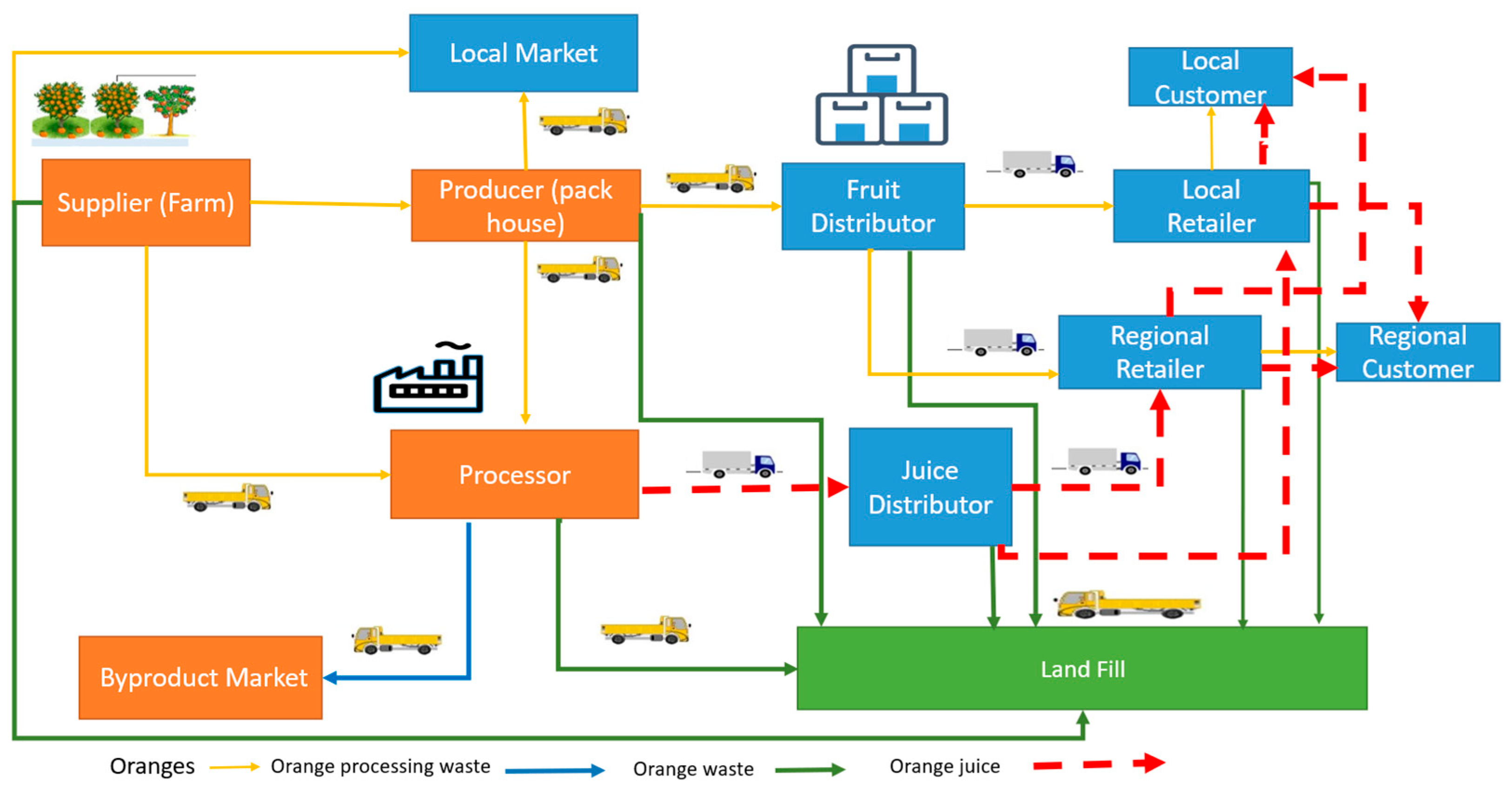
3.1. Citrus Supply Chain and Model Description

The citrus supply chain (CSC), illustrated in Figure 1, begins with suppliers, typically farms, harvesting citrus fruits. These suppliers sell fruits to either packhouses or processors. Fruits not meeting the quality standards of these entities are sold in local markets at a reduced price. The deteriorated fruit is wasted and sent to landfill. Upon arrival at the packhouse, fruits undergo quality inspection; low-quality fruits are sold in local markets, and deteriorated fruits are sent to landfills, whereas irregularly shaped and sized fruits are sold to processors, and the accepted fruits are directed to the production line at the packhouse. Production includes the washing, sorting, waxing, and finally packing of the fruit. Fruits can be dispatched directly to fruit distributors or stored in a refrigerated warehouse at the packhouse. Processors purchase fruits either directly from farms or packhouses. Incoming fruits that fail at the inspection stage are sent to landfill. The fruits are processed to extract juice, with approximately half of processed fruits yielding juice, and the other half comprising the citrus processing waste (CPW). The processor sells juice to juice distributors, while the CPW is sold in byproduct markets. The CPW can be either further processed to obtain value-added products or directly used as animal feed. Fruit and juice distributors sell their products to local or regional retailers. The products moving through the supply chain, including orange fruits, orange juice, fruit waste, and CPW, are measured in kilograms. The CSC was developed based on reviewing the supply chains introduced in previous research works. Moreover, it was verified by different CSC stakeholders in Egypt.

A mixed-integer linear programming (MILP) model is developed to optimize the CSC network design. The objective of the proposed model is to maximize total profit of the supply chain from farm to retailer. This global objective ensures coordination among all supply chain echelons. The model is applied before the start of the season to advise stakeholders on the optimal configuration of their supply chain, thereby increasing supply chain profit.

The proposed supply chain is considered both resilient and sustainable. Resilience is achieved through having multiple suppliers and facilities, a proactive resilience strategy that ensures operational flexibility across various echelons. Sustainability is addressed through its three pillars: economically, by maximizing supply chain profit; environmentally, by valorizing and selling CPW in byproduct markets instead of disposing it in landfills; and socially, by creating job opportunities for intermediaries or processors working on CPW.

The developed model determines the operational status of each facility, the quantities transported between all echelons, the processing quantities at packhouses and processors, and the inventory levels at each facility. Therefore, the model addresses both strategic decisions (number of facilities) and tactical decisions (supplier selection, allocation, inventory levels, and production quantities). The model incorporates constraints related to production capacities, inventory capacities, the flow balance of fruits and juice, demand satisfaction, waste quantities, and the quality of non-conforming fruits.

The model assumptions, indices, decision variables, objective function, and constraints are illustrated in the following sub-sections, while the model parameters are presented in

Table A1. Model parameters.

Supplier parameters
αsps	Selling price of one kg of fruit from supplier s to packhouse (LE/kg)
αscs	Selling price of one kg of fruit from supplier s to processer (LE/kg)
αsos	Selling price of one kg of fruit from supplier s to local market (LE/kg)
VCsst	Variable cost at supplier s in time t (LE/period)
ECsst	Energy cost at supplier s in time t (LE/period)
TRCsoso	Transportation cost from supplier s to local market o (LE/km/kg)
TRCslsl	Transportation cost from supplier s to landfill l (LE/km/kg)
Ysoso	Distance between supplier s and local market o (km)
Yslsl	Distance between supplier s and landfill l (km)
λsst	Production quantity at supplier s in time t (kgs/period)
θss	Percentage of fruit waste at supplier s (percent)
MQss	Percentage of non-conforming fruit going to local market from supplier s (percent)
Packhouse parameters
αpxp	Selling price of one kg of fruit from packhouse p to fruit distributor (LE/kg)
αpcp	Selling price of one kg of fruit from packhouse p to processor (LE/kg)
αpop	Selling price of one kg of fruit from packhouse p to local market (LE/kg)
VCppt	Variable cost at packhouse p in time t (LE/period)
MCppt	Maintenance cost at packhouse p in time t (LE/period)
ECppt	Energy cost at packhouse p in time t (LE/period)
TRCspsp	Transportation cost from supplier s to packhouse p (LE/km/kg)
TRCpopo	Transportation cost from packhouse p to local market o (LE/km/kg)
TRCplpl	Transportation cost from packhouse p to landfill l (LE/km/kg)
Yspsp	Distance between supplier s and packhouse p (km)
Ypopo	Distance between packhouse p and local market o (km)
Yplpl	Distance between packhouse p and landfill l (km)
hpp	Inventory holding cost of one kg of fruit at packhouse p (LE/kg)
θpp	Percentage of fruit waste at packhouse p (percent)
MQpp	Percentage of non-conforming fruit going to local market from packhouse p (percent)
λhpp	Holding inventory capacity at packhouse p (kgs)
λppt	Production capacity at packhouse p in time t (kgs/period)
Processor parameters
αcyc	Selling price of juice from processor c to fruit distributor (LE/kg)
αcbc	Selling price of juice processing waste from processor c to byproduct market (LE/kg)
VCcct	Variable cost at processor c in time t (LE/period)
MCcct	Maintenance cost at processor c in time t (LE/period)
ECcct	Energy cost at processor c in time t (LE/period)
TRCscsc	Transportation cost from supplier s to processor c (LE/km/kg)
TRCpcpc	Transportation cost from packhouse p to processor c (LE/km/kg)
TRCclcl	Transportation cost from processor c to landfill l (LE/km/kg)
Yscsc	Distance between supplier s and processor c (km)
Ypcpc	Distance between packhouse p and processor c (km)
Yclcl	Distance between processor c and landfill l (km)
hcc	Inventory holding cost per unit of juice at processor c (LE/kg)
θcc	Percentage of fruit waste at processor c (percent)
λhcc	Holding inventory capacity at processor c (kgs)
λcct	Production capacity at processor c in time t (kgs/period)
Fruit distributor parameters
αxrx	Selling price of one kg of fruit from fruit distributor x to local retailer (LE/kg)
αxqx	Selling price of one kg of fruit from fruit distributor x to regional retailer (LE/kg)
Wx	Wages at fruit distributor (LE/kg)
MCxxt	Maintenance cost at fruit distributor x in time t (LE/period)
ECxxt	Energy cost at fruit distributor x in time t (LE/period)
hxx	Inventory holding cost of one kg of fruit at fruit distributor x (LE/kg)
TRCpxpx	Transportation cost from packhouse p to fruit distributor x (LE/km/kg)
TRCxlxl	Transportation cost from fruit distributor x to landfill l (LE/km/kg)
Ypxpx	Distance between packhouse p and fruit distributor x (km)
Yxlxl	Distance between fruit distributor x and landfill l (km)
θxx	Percentage of the fruit waste at fruit distributor x (percent)
λhxx	Holding inventory capacity at fruit distributor x (kgs)
Juice distributor parameters
αyry	Selling price of juice from juice distributor y to local retailer (LE/kg)
αyqy	Selling price of juice from juice distributor y to regional retailer (LE/kg)
Wy	Wages at juice distributor (LE/kg)
MCyyt	Maintenance cost at juice distributor y in time t (LE/period)
ECyyt	Energy cost at juice distributor y in time t (LE/period)
TRCcycy	Transportation cost from processor c to juice distributor y (LE/km/kg)
Ycycy	Distance between processor c and juice distributor y (km)
hyy	Inventory holding cost per unit of juice at juice distributor y (LE/kg)
λhyy	Holding inventory capacity at juice distributor y (kgs)
Local retailer parameters
αfrr	Selling price of one kg of fruit at local retailer r (LE/kg)
αjrr	Selling price of one kg of juice at local retailer r (LE/kg)
Dfrrt	Demand for fruit at local retailer r in time t (kg/period)
Djrrt	Demand for juice at local retailer r in time t (kg/period)
Wr	Wages at local retailer (LE/kg)
MCrrt	Maintenance cost at local retailer r in time t (LE/period)
ECrrt	Energy cost at local retailer r in time t (LE/period)
TRCxrxr	Transportation cost from fruit distributor x to local retailer r (LE/km/kg)
TRCyryr	Transportation cost from juice distributor y to local retailer r (LE/km/kg)
TRCrlrl	Transportation cost from local retailer r to landfill l (LE/km/kg)
Yxrxr	Distance between fruit distributor x and local retailer r (km)
Yyryr	Distance between from juice distributor y and local retailer r (km)
Yrlrl	Distance between local retailer r and landfill l (km)
hrr	Inventory holding cost per unit at local retailer r (LE/kg)
θrr	Percentage of the fruit waste at local retailer r (percent)
λhfrr	Holding inventory capacity of fruit at local retailer r (kgs)
λhjrr	Holding inventory capacity of juice at local retailer r (kgs)
Regional retailer parameters
αfqq	Selling price of one kg of fruit at regional retailer q (LE/kgs)
αjqq	Selling price of one kg of juice at regional retailer q (LE/kgs)
Dfqqt	Demand for fruit at regional retailer q in time t (kg/period)
Djqqt	Demand for juice at regional retailer q in time t (kg/period)
Wq	Wages at regional retailer (LE/kg)
MCqqt	Maintenance cost at regional retailer q in time t (LE/period)
ECqqt	Energy cost at regional retailer q in time t (LE/period)
TRCxqxq	Transportation cost from fruit distributor x to regional retailer q (LE/km/kg)
TRCyqyq	Transportation cost from juice distributor y to regional retailer q (LE/km/kg)
TRCqlql	Transportation cost from regional retailer q to landfill l (LE/km/kg)
Yxqxq	Distance between fruit distributor x and regional retailer q (km)
Yyqyq	Distance between from juice distributor y and regional retailer q (km)
Yqlql	Distance between regional retailer q and landfill l (km)
hqq	Inventory holding cost per unit at regional retailer q (LE/kg)
θqq	Percentage of the fruit waste at regional retailer q (percent)
λhfqq	Holding inventory capacity of fruit at regional retailer q (kgs)
λhjqq	Holding inventory capacity of juice at regional retailer q (kgs)
Abbreviations
DC	Cost of waste disposal for one kg of fruit (LE/kg)
M	Big value
Auxiliary variables
PS	Profits of suppliers (LE)
REVSst	Revenue at supplier s in time t (LE/period)
TCSst	Total cost at supplier s in time t (LE/period)
COTSst	Transportation cost related to supplier s in time t (LE/period)
PP	Profits of packhouses (LE)
REVPpt	Revenue at packhouse p in time t (LE/period)
TCPpt	Total cost at packhouse p in time t (LE/period)
PCPpt	Purchasing cost at packhouse p in time t (LE/period)
COTPpt	Transportation cost related to packhouse p in time t (LE/period)
HCPpt	Holding cost at packhouse p in time t (LE/period)
PC	Profits of processors (LE)
REVCct	Revenue at processor c in time t (LE/period)
TCCct	Total cost at processor c in time t (LE/period)
PCCct	Purchasing cost at processor c in time t (LE/period)
COTCct	Transportation cost related to processor c in time t (LE/period)
HCCct	Holding cost at processor c in time t (LE/period)
PX	Profits of fruit distributors (LE)
REVXxt	Revenue at fruit distributor x in time t (LE/period)
TCXxt	Total cost at fruit distributor x in time t (LE/period)
PCXxt	Purchasing cost at fruit distributor x in time t (LE/period)
COTXxt	Transportation cost related to fruit distributor x in time t (LE/period)
HCXxt	Holding cost at fruit distributor x in time t (LE/period)
PY	Profits of juice distributors (LE)
REVYyt	Revenue at juice distributor y in time t (LE/period)
TCYyt	Total cost at juice distributor y in time t (LE/period)
PCYyt	Purchasing cost at juice distributor y in time t (LE/period)
COTYyt	Transportation cost related to juice distributor y in time t (LE/period)
HCYyt	Holding cost at juice distributor y in time t (LE/period)
PR	Profits of local retailers (LE)
REVRrt	Revenue at local retailer r in time t (LE/period)
TCRrt	Total cost at local retailer r in time t (LE/period)
PCRrt	Purchasing cost at local retailer r in time t (LE/period)
COTRrt	Transportation cost related to local retailer r in time t (LE/period)
HCRrt	Holding cost at local retailer r in time t (LE/period)
PQ	Profits of regional retailers (LE)
REVQqt	Revenue at regional retailer q in time t (LE/period)
TCQqt	Total cost at regional retailer q in time t (LE/period)
PCQqt	Purchasing cost at regional retailer q in time t (LE/period)
COTQqt	Transportation cost related to regional retailer q in time t (LE/period)
HCQqt	Holding cost at regional retailer q in time t (LE/period)

in Appendix A.

3.2. Model Assumptions

The following assumptions are considered:

• The return flows of products are not considered.
• The CPW is assumed to be sent to one byproduct market, although different byproducts are generated. This is because the CPW can be sold as animal feed, for example.
• The demand is deterministic, according to the forecasted quantities.
• No backorders are allowed, and all demand should be met.
• Wages are considered the same for all stakeholders in the same echelon and depend on the number of units produced.
• Inventory costs at retailers are the same for both fruit and juice, since they are stored in a refrigerated space, and they take up almost the same area.
• Transportation vehicles among stakeholders have unlimited capacity since they are outsourced.

3.3. Model Indices

Table 5. Model indices.

s = 1, 2, …, S	Set of Farms	q = 1, 2, …, Q	Set of Regional Retailers
p = 1, 2, …, P	Set of Packhouses	o = 1, 2, …, O	Set of Local Markets
c = 1, 2, …, C	Set of Processors	b = 1, 2, …, B	Set of Byproduct Markets
x = 1, 2, …, X	Set of Orange Distributors	l = 1, 2, …, L	Set of Landfills
y = 1, 2, …, Y	Set of Juice Distributors	t = 1, 2, …, T	Set of Time Periods
r = 1, 2, …, R	Set of Local Retailers

presents the model indices.

3.4. Model Decision Variables

Table 6. Model decision variables.

NSPspt	Transported amounts of fruits from supplier s to packhouse p at time t (kgs/period)
NSCsct	Transported amounts of fruits from supplier s to processor c at time t (kgs/period)
NSOsot	Transported amounts of fruits from supplier s to local market o at time t (kgs/period)
NSLslt	Transported amounts of fruit waste from supplier s to landfill l at time t (kgs/period)
NPCpct	Transported amounts of fruits from packhouse p to processor c at time t (kgs/period)
NPXpxt	Transported amounts of fruits from packhouse p to fruit distributor x at time t (kgs/period)
NPOpot	Transported amounts of fruits from packhouse p to local market o at time t (kgs/period)
NPLplt	Transported amounts of fruit waste from packhouse p to landfill l at time t (kgs/period)
NCYcyt	Transported amounts of juice from processor c to juice distributor y at time t (kgs/period)
NCBcbt	Transported amounts of juice processing waste from processor c to byproduct market b at time t (kgs/period)
NCLclt	Transported amounts of fruit waste from processor c to landfill l at time t (kgs/period)
NXRxrt	Transported amounts of fruits from fruit distributor x to local retailer r at time t (kgs/period)
NXQxqt	Transported amounts of fruits from fruit distributor x to regional retailer q at time t (kgs/period)
NXLxlt	Transported amounts of fruit waste from fruit distributor x to landfill l at time t (kgs/period)
NYRyrt	Transported amounts of juice from juice distributor y to local retailer r at time t (kgs/period)
NYQyqt	Transported amounts of juice from juice distributor y to regional retailer q at time t (kgs/period)
NRLrlt	Transported amounts of fruit waste from local retailer r to landfill l at time t (kgs/period)
NQLqlt	Transported amounts of fruit waste from regional retailer r to landfill l at time t (kgs/period)
IPpt	Inventory level at packhouse p in time t (kgs/period)
ICct	Inventory level at processor c in time t (kgs/period)
IXxt	Inventory level at fruit distributor x in time t (kgs/period)
IYyt	Inventory level at juice distributor y in time t (kgs/period)
IFRrt	Inventory level of fruit at local retailer r in time t (kgs/period)
IJRrt	Inventory level of juice at local retailer r in time t (kgs/period)
IFQqt	Inventory level of fruit at regional retailer r in time t (kgs/period)
IJQqt	Inventory level of juice at regional retailer r in time t (kgs/period)
$\sigma$Ppt	Packed amounts of fruits at packhouse p at time t (kgs/period)
$\sigma$Cct	Processed amounts of fruits at processor c at time t (kgs/period)
EJct	Extracted amount of juice from processing of 1 kg of oranges at processor c in time t (kgs/period)
EBct	Extracted amount of CPW from processing of 1 kg of oranges at processor c in time t (kgs/period)
BSst	1 if supplier s in time t is functioning, otherwise 0
BPpt	1 if packhouse p in time t is functioning, otherwise 0
BCct	1 if processor c in time t is functioning, otherwise 0
BXxt	1 if fruit distributor x in time t is functioning, otherwise 0
BYyt	1 if juice distributor y in time t is functioning, otherwise 0
BRrt	1 if local retailer r in time t is functioning otherwise 0
BQqt	1 if regional retailer q in time t is functioning, otherwise 0

shows the model decision variables.

3.5. Model Objective Function

The objective of the proposed model (1) is to maximize the complete supply chain profit (SCP). This profit is calculated based on aggregate profits of all echelons within the supply chain in all periods. The profit of each echelon (2, 6, 12, 18, 24, 30, 36) is determined by the difference between its revenue and its total costs.

Max SCP = PS + PP + PC + PX + PY + PR + PQ

(1)

The total revenues for a supplier (3) are derived from selling fruits to packhouses, processors, or local markets. The total costs for a supplier (4) encompass variable costs, energy costs, transportation costs, and disposal costs. The total cost of transportation (5) is calculated based on the quantity transported to local markets and landfills, the unit price of transport, and the traveled distance.

$$PS=\sum _{t=1}^T\sum _{s=1}^S{REVS}_{st}-\sum _{t=1}^T\sum _{s=1}^S{TCS}_{st}$$

(2)

$${REVS}_{st}=\sum _{p=1}^P{\alpha sp}_s\ast {NSP}_{spt}+\sum _{c=1}^C{\alpha sc}_s\ast {NSC}_{sct}+\sum _{o=1}^O{{bs}_{st}\ast \alpha so}_s\ast {NSO}_{sot}$$

(3)

$${TCS}_{st}={BS}_{st}\ast \left({VCs}_{st}+{ECs}_{st}+{COTS}_{st}+\sum _{l=1}^L{NSL}_{slt}\ast DC\right)$$

(4)

$${COTS}_{st}=\sum _{o=1}^O{TRCso}_{so}\ast {Yso}_{so}\ast {NSO}_{sot}+\sum _{l=1}^L{TRCsl}_{sl}\ast {Ysl}_{sl}\ast {NSL}_{slt}$$

(5)

The total revenues for a packhouse (7) are generated by selling packed fruits to processors, fruit distributors, or local markets. The total costs for a packhouse (8) include the same categories as those for a supplier, with additional costs for purchasing, maintenance, and inventory. The purchasing costs (9) are calculated based on the quantities transported from suppliers. The transportation costs (10) are the costs of the open trucks used to deliver fruits to local markets and landfills, and transport fruits from suppliers. The inventory holding costs (11) are determined based on stored quantities.

$$PP=\sum _{t=1}^T\sum _{p=1}^P{REVP}_{pt}-\sum _{t=1}^T\sum _{p=1}^P{TCP}_{pt}$$

(6)

$${REVP}_{pt}=\sum _{c=1}^C{\alpha pc}_p\ast {NPC}_{pct}+\sum _{x=1}^X{\alpha px}_p\ast {NPX}_{pxt}+\sum _{o=1}^O{\alpha po}_p\ast {NPO}_{pot}$$

(7)

$${TCP}_{pt}={BP}_{pt}\ast \left({PCP}_{pt}+{VCp}_{pt}+{MCp}_{pt}+{ECp}_{pt}+{COTP}_{pt}+{HCP}_{pt}+\sum _{l=1}^L{NPL}_{plt}\ast DC\right)$$

(8)

$${PCP}_{pt}=\sum _{s=1}^S{\alpha sp}_s\ast {NSP}_{spt}$$

(9)

$${COTP}_{pt}=\sum _{s=1}^S{TRCsp}_{sp}\ast {Ysp}_{sp}\ast {NSP}_{spt}+\sum _{o=1}^O{TRCpo}_{po}\ast {Ypo}_{po}\ast {NPO}_{pot}+\sum _{l=1}^L{TRCpl}_{pl}\ast {Ypl}_{pl}\ast {NPL}_{plt}$$

(10)

$${HCP}_{pt}={hp}_p\ast {IP}_{pt}$$

(11)

The total revenues for a processor (13) are derived from selling juice to juice distributors and CPW to byproduct markets. The total costs (14), purchasing costs (15), transportation costs (16), and holding costs (17) for a processor are calculated similarly to those of a packhouse.

$$PC=\sum _{t=1}^T\sum _{c=1}^C{REVC}_{ct}-\sum _{t=1}^T\sum _{c=1}^C{TCC}_{ct}$$

(12)

$${REVC}_{ct}=\sum _{y=1}^Y{\alpha cy}_c\ast {NCY}_{cyt}+\sum _{b=1}^B{\alpha cb}_c\ast {NCB}_{cbt}$$

(13)

$${TCC}_{ct}={BC}_{ct}\ast \left({PCC}_{ct}+{VCc}_{ct}+{MCc}_{ct}+{ECc}_{ct}+{COTC}_{ct}+{HCC}_{ct}+\sum _{l=1}^L{NCL}_{clt}\ast DC\right)$$

(14)

$${PCC}_{ct}=\sum _{p=1}^P{\alpha pc}_p\ast {NPC}_{pct}+\sum _{s=1}^S{\alpha sc}_s\ast {NSC}_{sct}$$

(15)

$${COTC}_{ct}=\sum _{s=1}^S{TRCsc}_{sc}\ast {Ysc}_{sc}\ast {NSC}_{sct}+\sum _{p=1}^P{TRCpc}_{pc}\ast {Ypc}_{pc}\ast {NPC}_{pct}+\sum _{l=1}^L{TRCcl}_{cl}\ast {Ycl}_{cl}\ast {NCL}_{clt}$$

(16)

$${HCC}_{ct}={hc}_c\ast {IC}_{ct}$$

(17)

The total revenues for a fruit distributor (19) are generated by selling packed fruits to local or regional retailers. The total costs for a fruit distributor (20) include expenses for purchasing, wages, maintenance, energy, transportation, inventory, and disposal. The purchasing costs (21), transportation costs (22), and holding costs (23) for a fruit distributor are calculated similarly to those of a processor.

$$PX=\sum _{t=1}^T\sum _{x=1}^X{REVX}_{xt}-\sum _{t=1}^T\sum _{x=1}^X{TCX}_{xt}$$

(18)

$${REVX}_{xt}=\sum _{r=1}^R{\alpha xr}_x\ast {NXR}_{xrt}+\sum _{q=1}^Q{\alpha xq}_x\ast {NXQ}_{xqt}$$

(19)

$${TCX}_{xt}={BX}_{xt}\ast ({PCX}_{xt}+\sum _{p=1}^{P}Wx\ast {NPX}_{pxt}+{MCx}_{xt}+{ECx}_{xt}+{COTX}_{xt}+{HCX}_{xt}+\sum _{l=1}^L{NXL}_{xlt}\ast DC)$$

(20)

$${PCX}_{xt}=\sum _{p=1}^P{\alpha px}_p\ast {NPX}_{pxt}$$

(21)

$${COTX}_{xt}=\sum _{p=1}^P{TRCpx}_{px}\ast {Ypx}_{px}\ast {NPX}_{pxt}+\sum _{l=1}^L{TRCxl}_{xl}\ast {Yxl}_{xl}\ast {NXL}_{xlt}$$

(22)

$${HCX}_{xt}={hx}_x\ast {IX}_{xt}$$

(23)

The total revenues for a juice distributor (25) are obtained from selling juice to local and regional retailers. The total costs for a juice distributor (26) are like those of a fruit distributor, excluding disposal costs, as expired juice is not disposed of in landfills. The purchasing costs (27), transportation costs (28), and holding costs (29) are calculated similarly to those of a fruit distributor.

$$PY=\sum _{t=1}^T\sum _{y=1}^Y{REVY}_{yt}-\sum _{t=1}^T\sum _{y=1}^Y{TCY}_{yt}$$

(24)

$${REVY}_{yt}=\sum _{r=1}^R{\alpha yr}_y\ast {NYR}_{yrt}+\sum _{q=1}^Q{\alpha yq}_y\ast {NYQ}_{yqt}$$

(25)

$${TCY}_{yt}={BY}_{yt}\ast \left({PCY}_{yt}+\sum _{c=1}^{C}Wy\ast {NCY}_{cyt}+{MCy}_{yt}+{ECy}_{yt}+{COTY}_{yt}+{HCY}_{yt}\right)$$

(26)

$${PCY}_{yt}=\sum _{c=1}^C{\alpha cy}_c\ast {NCY}_{cyt}$$

(27)

$${COTY}_{yt}=\sum _{c=1}^C{TRCcy}_{cy}\ast {Ycy}_{cy}\ast {NCY}_{cyt}$$

(28)

$${HCY}_{yt}={hy}_y\ast {IY}_{yt}$$

(29)

The total revenues for a local retailer (31) are generated by selling fruit and juice to local customers. The total costs for a local retailer (32) encompass expenses for purchasing, wages, maintenance, energy, transportation, inventory, and disposal. The purchasing costs (33), transportation costs (34), and holding costs (35) are calculated similarly to those of the juice distributor.

$$PR=\sum _{t=1}^T\sum _{r=1}^R{REVR}_{rt}-\sum _{t=1}^T\sum _{r=1}^R{TCR}_{rt}$$

(30)

$${REVR}_{rt}=\left({\alpha fr}_r\ast {Dfr}_{rt}\right)+\left({\alpha jr}_r\ast {Djr}_{rt}\right)$$

(31)

$${TCR}_{rt}={BR}_{rt}\ast \left({PCR}_{rt}+\sum _{x=1}^{X}Wr\ast {NXR}_{xrt}+\sum _{y=1}^{Y}Wr\ast {NYR}_{yrt}+{MCr}_{rt}+{ECr}_{rt}+{COTR}_{rt}+{HCR}_{rt}+\sum _{l=1}^L{NRL}_{rlt}\ast DC\right)$$

(32)

$${PCR}_{rt}=\sum _{x=1}^X{\alpha xr}_x\ast {NXR}_{xrt}+\sum _{y=1}^Y{\alpha yr}_y\ast {NYR}_{yrt}$$

(33)

$${COTR}_{rt}=\sum _{x=1}^X{TRCxr}_{xr}\ast {Yxr}_{xr}\ast {NXR}_{xrt}+\sum _{y=1}^Y{TRCyr}_{yr}\ast {Yyr}_{yr}\ast {NYR}_{yrt}+\sum _{l=1}^L{TRCrl}_{rl}\ast {Yrl}_{rl}\ast {NRL}_{rlt}$$

(34)

$${HCR}_{rt}={hr}_r\ast \left({IFR}_{rt}+{IJR}_{rt}\right)$$

(35)

The total revenues for a regional retailer (37) are derived from selling fruits and juice to regional customers. The remaining cost equations (38–41) are identical to those of a local retailer.

$$PQ=\sum _{t=1}^T\sum _{q=1}^Q{REVQ}_{qt}-\sum _{t=1}^T\sum _{q=1}^Q{TCQ}_{qt}$$

(36)

$${REVQ}_{qt}=\left({\alpha fq}_q\ast {Dfq}_{qt}\right)+\left({\alpha jq}_q\ast {Djq}_{qt}\right)$$

(37)

$${TCQ}_{qt}={BQ}_{qt}\ast ({PCQ}_{qt}+\sum _{x=1}^{X}Wq\ast {NXQ}_{xqt}+\sum _{y=1}^{Y}Wq\ast {NYQ}_{yqt}+{MCq}_{qt}+{ECq}_{qt}+{COTQ}_{qt}+{HCQ}_{qt}+\sum _{l=1}^L{NQL}_{qlt}\ast DC)$$

(38)

$${PCQ}_{qt}=\sum _{x=1}^X{\alpha xq}_x\ast {NXQ}_{xqt}+\sum _{y=1}^Y{\alpha yq}_y\ast {NYQ}_{yqt}$$

(39)

$${COTQ}_{qt}=\sum _{x=1}^X{TRCxq}_{xq}\ast {Yxq}_{xq}\ast {NXQ}_{xqt}+\sum _{y=1}^Y{TRCyq}_{yq}\ast {Yyq}_{yq}\ast {NYQ}_{yqt}+\sum _{l=1}^L{TRCql}_{ql}\ast {Yql}_{ql}\ast {NQL}_{qlt}$$

(40)

$${HCQ}_{qt}={hq}_q\ast \left({IFQ}_{qt}+{IJQ}_{qt}\right)$$

(41)

3.6. Model Constraints

Supplier Constraints

$${\lambda s}_{st}\ge \sum _{p=1}^P{NSP}_{spt}+\sum _{c=1}^C{NSC}_{sct}+\sum _{o=1}^{O}N{SO}_{sot}+\sum _{l=1}^{L}N{SL}_{slt}\hspace{1em}\forall s,t$$

(42)

$$\sum _{l=1}^L{NSL}_{slt}={\theta s}_s\ast {\lambda s}_{st}\hspace{1em}\forall s,t$$

(43)

$$\sum _{o=1}^O{NSO}_{sot}\le {MQs}_s\ast {\lambda s}_{st}\hspace{1em}\forall s,t$$

(44)

$$\sum _{p=1}^P{NSP}_{spt}+\sum _{c=1}^C{NSC}_{sct}\le M\ast {BS}_{st}\hspace{1em}\forall s,t$$

(45)

Constraint (42) ensures that the quantities transported to packhouses, processors, local markets, and landfills do not exceed the quantity produced by the supplier (farm). Constraints (43) and (44) determine the transported quantities to landfills or local markets as a percentage of the farm’s production quantity. Finally, constraint (45) ensures that if a supplier is not chosen, its costs and revenues are not considered.

Packhouse Constraints

$${IP}_{pt}={\sigma P}_{pt}+\left({IP}_{pt}-1\right)-\sum _{x=1}^X{NPX}_{pxt}-\sum _{c=1}^C{NPC}_{pct}\hspace{1em}\forall p,t$$

(46)

$${\sigma P}_{pt}=\sum _{s=1}^S{NSP}_{spt}-\sum _{0 =1}^{O}N{PO}_{pot}-\sum _{l=1}^{L}N{PL}_{plt}\hspace{1em}\forall p,t$$

(47)

$$\sum _{o=1}^{O}N{PO}_{pot}\le {MQp}_p\ast \sum _{s=1}^{S}N{SP}_{spt}\hspace{1em}\forall p,t$$

(48)

$$\sum _{l=1}^{L}N{PL}_{plt}={\theta p}_p\ast \sum _{s=1}^S{NSP}_{spt}\hspace{1em}\forall p,t$$

(49)

$${IP}_{pt}\le \lambda {hp}_p\hspace{1em}\forall p,t$$

(50)

$${\sigma P}_{pt}\le {\lambda p}_{pt}\hspace{1em}\forall p,t$$

(51)

$${\sigma P}_{pt}\le M\ast {BP}_{pt}\hspace{1em}\forall p,t$$

(52)

Constraint (46) ensures the flow balance at packhouses. The stored quantities at time t must be equal to the quantities transported to fruit distributors and processors, subtracted from the packed quantities of fruits in the packhouse and the stored quantities in the inventory from the previous period. Constraint (47) states that the quantities of fruits packed at the packhouse must be equal to the quantities transported to local markets and landfills, deducted from the quantities received at the packhouse from all suppliers. Constraints (48) and (49) determine the quantities transported to local markets and landfills as a percentage of all quantities received at the packhouse from all suppliers. The inventory level and packed quantities of fruits are constrained by the packhouse’s holding and production capacities, respectively (constraints (50) and (51)). Finally, constraint (52) guarantees that if a packhouse is not selected, then its costs and revenues are not counted.

Processor Constraints

$${IC}_{ct}={EJ}_{ct}+\left({IC}_{ct}-1\right)-\sum _{y=1}^Y{NCY}_{cyt}\hspace{1em}\forall c,t$$

(53)

$${\sigma C}_{ct}=\left(1-{\theta c}_c\right)\ast \left(\sum _{s=1}^S{NSC}_{sct}+\sum _{p=1}^P{NPC}_{pct}\right)\hspace{1em}\forall c,t$$

(54)

$${EJ}_{ct}=0.5\ast {\sigma C}_{ct}\hspace{1em}\forall c,t$$

(55)

$${EB}_{ct}=0.5\ast {\sigma C}_{ct}\hspace{1em}\forall c,t$$

(56)

$$\sum _{b=1}^B{NCB}_{cbt}={EB}_{ct}\hspace{1em}\forall c,t$$

(57)

$$\sum _{l=1}^{L}N{CL}_{clt}={\theta c}_c\ast \left(\sum _{s=1}^S{NSC}_{sct}+\sum _{p=1}^{P}N{PC}_{pct}\right)\hspace{1em}\forall c,t$$

(58)

$${IC}_{ct}\le {\lambda hc}_c\hspace{1em}\forall c,t$$

(59)

$${\sigma C}_{ct}\le {\lambda c}_{ct}\hspace{1em}\forall c,t$$

(60)

$${\sigma C}_{ct}\le M\ast {BC}_{ct}\hspace{1em}\forall c,t$$

(61)

Constraint (53) provides the flow balance at the processors. The stored quantities at time t must be equal to the extracted amounts of juice at the processor and the quantities stored in the inventory from the previous period minus the transported quantities to the juice distributors. Constraint (54) ensures that processed quantities of fruits at the processor should be equal to the transported quantities from suppliers and packhouses, adjusted according to the waste removed due to the incoming inspection process. The following two constraints (55) and (56) calculate the extracted amounts of juice and CPW as a proportion of the processed quantities of fruits at the processor. Constraints (57) and (58) define the transported quantities to byproduct markets and landfills. Constraints (59) and (60) limit the stored and processed quantities at the packhouse. Finally, constraint (61) ensures that if a processor is not selected, then its costs and revenues are not calculated.

Fruit Distributor Constraints

$${IX}_{xt}=\sum _{p=1}^P{NPX}_{pxt}+\left({IX}_{xt}-1\right)-\sum _{r=1}^R{NXR}_{xrt}-\sum _{q=1}^{Q}N{XQ}_{xqt}-\sum _{l=1}^L{NXL}_{xlt}\hspace{1em}\forall x,t$$

(62)

$$\sum _{l=1}^L{NXL}_{xlt}={\theta x}_x\ast \sum _{p=1}^P{NPX}_{pxt}\hspace{1em}\forall x,t$$

(63)

$${IX}_{xt}\le {\lambda hx}_x \hspace{1em}\forall x,t$$

(64)

$$\sum _{r=1}^R{NXR}_{xrt}+\sum _{q=1}^{Q}N{XQ}_{xqt}\le M\ast {BX}_{xt}\hspace{1em}\forall x,t$$

(65)

Constraint (62) ensures that the flow balance at the fruit distributors is maintained. The stored quantities at time t must equal to the transported quantities to local retailers, regional retailers, and landfills, subtracted from the received quantities at the fruit distributor and the stored quantities in the inventory from the previous period. Constraint (63) specifies the quantities transported to landfills as a percentage of the quantities received at the fruit distributor from all packhouses. Constraint (64) checks that the inventory level does not exceed the holding inventory capacity of the fruit distributor. Finally, constraint (65) guarantees that if a fruit distributor is not selected, then its costs and revenues are not calculated.

Juice Distributor Constraints

$${IY}_{yt}=\sum _{c=1}^C{NCY}_{cyt}+\left({IY}_{yt}-1\right)-\sum _{r=1}^{R}N{YR}_{yrt}-\sum _{q=1}^Q{NYQ}_{yqt}\hspace{1em}\forall y,t$$

(66)

$${IY}_{yt}\le {\lambda hy}_y\hspace{1em}\forall y,t$$

(67)

$$\sum _{r=1}^{R}N{YR}_{yrt}+\sum _{q=1}^Q{NYQ}_{yqt}\le M\ast {BY}_{yt}\hspace{1em}\forall y,t$$

(68)

Constraint 66 ensures flow balance at the juice distributor. Constraint (67) limits the stored quantities at the juice distributors. Finally, constraint (68) ensures that if a juice distributor is not selected, then its costs and revenues are not calculated.

Local Retailer Constraints

$${IFR}_{rt}=\sum _{x=1}^X{NXR}_{xrt}+\left({IFR}_{rt}-1\right)-{Dfr}_{rt}-\sum _{l=1}^L{NRL}_{rlt}\hspace{1em}\forall r,t$$

(69)

$${IJR}_{rt}=\sum _{y=1}^Y{NYR}_{yrt}+\left({IJR}_{rt}-1\right)-{Djr}_{rt}\hspace{1em}\forall r,t$$

(70)

$$\sum _{l=1}^L{NRL}_{rlt}={\theta r}_r\ast \sum _{x=1}^X{NXR}_{xrt}\hspace{1em}\forall r,t$$

(71)

$${IFR}_{rt}\le {\lambda hfr}_r\hspace{1em}\forall r,t$$

(72)

$${IJR}_{rt}\le {\lambda hjr}_r\hspace{1em}\forall r,t$$

(73)

$$\sum _{x=1}^X{NXR}_{xrt}+\sum _{y=1}^Y{NYR}_{yrt}\le M\ast {BR}_{rt}\hspace{1em}\forall r,t$$

(74)

The first two constraints (69) and (70) provide the flow balance of fruits and juice at local retailers. The stored quantities of fruits at time t should match fruits’ demand at the local retailer and the quantities transported to landfills, subtracted from the incoming quantities from fruit distributors and stored quantities in the inventory from the previous period. Similarly, the flow balance for juice is attained. Constraint (71) assures that transported quantities to landfills are determined as a percentage of the quantities of fruits received from all fruit distributors. Constraints (72) and (73) guarantee that the inventory levels of both products (fruit and juice) do not exceed the holding inventory capacity of the local retailer. Finally, constraint (74) guarantees that if a local retailer is not selected, then its costs and revenues are not considered.

Regional Retailer Constraints

$${IFQ}_{qt}=\sum _{x=1}^X{NXQ}_{xqt}+\left({IFQ}_{qt}-1\right)-{Dfq}_{qt}-\sum _{l=1}^L{NQL}_{qlt}\hspace{1em}\forall q,t$$

(75)

$${IJQ}_{qt}=\sum _{y=1}^Y{NYQ}_{yqt}+\left({IJQ}_{qt}-1\right)-{Djq}_{qt}\hspace{1em}\forall q,t$$

(76)

$$\sum _{l=1}^{L}N{QL}_{qlt}={\theta q}_q\ast \sum _{x=1}^X{NXQ}_{xqt}\hspace{1em}\forall q,t$$

(77)

$${IFQ}_{qt}\le {\lambda hfq}_q\hspace{1em}\forall q,t$$

(78)

$${IJQ}_{qt}\le {\lambda hjq}_q\hspace{1em}\forall q,t$$

(79)

$$\sum _{x=1}^X{NXQ}_{xqt}+\sum _{y=1}^Y{NYQ}_{yqt}\le M\ast {BQ}_{qt}\hspace{1em}\forall q,t$$

(80)

The regional retailers’ constraints (75–80) are similar to local retailers’ constraints.

Non-Negativity and Binary Constraints

$${NSP}_{spt}\ge 0 N{SO}_{sot}\ge 0 N{SC}_{sct}\ge 0 N{SL}_{slt}\ge 0 N{PC}_{pct}\ge 0 {NPX}_{pxt}\ge 0 N{PO}_{pot}\ge 0 {NPL}_{plt}\ge 0 {NCY}_{cyt}\ge 0 N{CB}_{cbt}\ge 0 N{CL}_{clt}\ge 0 N{XR}_{xrt}\ge 0 N{XQ}_{xqt}\ge 0 N{XL}_{xlt}\ge 0 N{YR}_{yrt}\ge 0 N{YQ}_{yqt}\ge 0 N{RL}_{rlt}\ge 0 N{QL}_{qlt}\ge 0 \hspace{1em}\forall s,p,c,x,y,r,q,t$$

(81)

$${\sigma P}_{pt}\ge 0 {\sigma C}_{ct}\ge 0 \hspace{1em}\forall p,c,t$$

(82)

$${IP}_{pt}\ge 0 {IC}_{ct}\ge 0 I{X}_{xt}\ge 0 {IY}_{yt}\ge 0 \hspace{1em}\forall p,c,x,y,t$$

(83)

$${IFR}_{rt}\ge 0 {IJR}_{rt}\ge 0 {IFQ}_{qt}\ge 0 {IJQ}_{qt}\ge 0 \hspace{1em}\forall r,q,t$$

(84)

$${BS}_{st},{BP}_{pt},{BC}_{ct},{BX}_{xt},{BY}_{yt},{BR}_{rt},{BQ}_{qt}\in \left\{0,1\right\}\hspace{1em}\forall s,p,c,x,y,r,q,t$$

(85)

4. Model Application

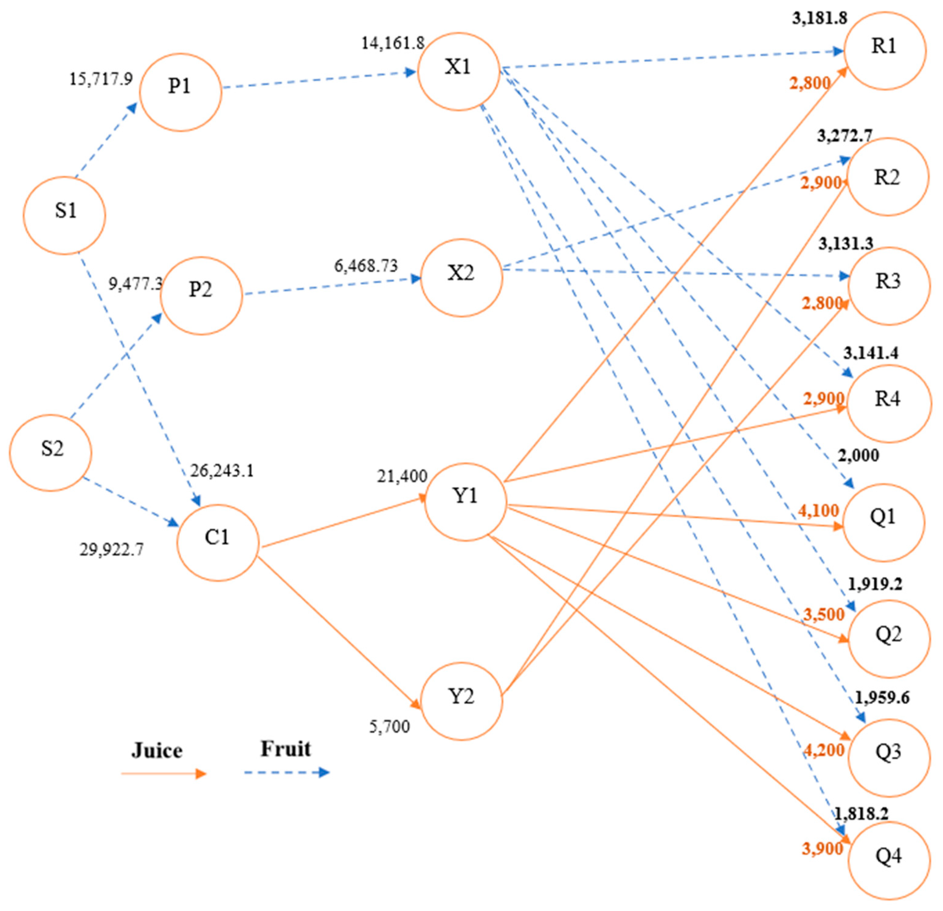
4.1. Complete Citrus Supply Chain

A citrus supply chain (CSC) scenario in Egypt, including citrus fruit and juice, is developed to justify the applicability of proposed model. The supply chain encompasses three suppliers, two packhouses, two processors, four local retailers, and four regional retailers. Each retailer represents multiple outlets within a specific zone to accurately reflect the supply chain dynamics. The time period is considered as one week, and the model is applied for two time periods. Two time periods are considered as a sample of the season to illustrate the applicability of the proposed model, as collecting and verifying large datasets over multiple periods can introduce inconsistencies and complexity. Applying the model on two time periods involves more than 500 parameters and 310 decision variables. The input data for running the model is obtained from the following CSC stakeholders in Egypt: two farms, two processors, two packhouses, one distributor, one exporter, two byproduct producers, and two retailers. Data are collected through personal interviews with owners or managers, then filtered and added in a table form and sent back to the stakeholders for verification. These data are supplemented by data gathered from research papers to address any missing data. Distances are calculated with the aid of Google maps using the specific locations of stakeholders. The main output of the developed model is an optimum CSC network design, which maximizes supply chain profit and considers resilience and sustainability aspects.

To design a resilient supply chain network, a couple of resilience strategies suggested in earlier studies are evaluated to mitigate expected disruptions at the supplier, packhouse, processor, and transportation echelons. Numerous types of disruptions can occur along the CSC; however, the developed model is being applied to a CSC in Egypt. Thus, the selection of disruptions to study at certain echelons is based on interviews with different stakeholders in the Egyptian citrus market. The studied disruptions are assumed to occur at the beginning of the study period. The model outputs of different scenarios are analyzed to identify the most effective resilience strategy to cope with expected disruptions occurring at different echelons. To aid in determining the best resilience strategy, supply chain resilience is calculated and used as a performance measure. It is measured using a simplified version of the method proposed by S. Zhao & You [43]. It is calculated as the ratio between the supply chain profit before and after the occurrence of disruption. Having a high ratio implies that the applied mitigation strategy has led to the supply chain profit (the main objective of supply chain) not being very affected after the occurrence of disruption at a certain echelon.

Supplier disruptions can arise from extreme weather conditions or from pandemics, such as COVID-19 for example. To determine the most appropriate strategy in case of supplier disruptions, three scenarios (runs) are tested. In Run 1, one of the suppliers (S1) experiences a complete disruption and thus has zero production capacity. As the other suppliers are not disrupted, this scenario represents having a multi-supplier strategy. In Run 2, an additional supplier (S4) with a different production capacity is introduced as a reactive resilience strategy to disruptions occurring at S1. S4 has a limited capacity and offers its products at a higher selling price. Run 3 represents a complete disruption (zero production capacity) to two suppliers, S1 and S2. This scenario represents having a sole supplier (S3); accordingly, no resilience strategy is applied.

Disruptions at packhouses can occur due to numerous factors, including machinery failure, limited fuel availability, electricity shortages, or pandemic events such as COVID-19. These disruptions can lead to facility shutdowns or reduced working hours. To successfully manage these disruptions, it is vital to adopt strategies that increase flexibility in production capacity. To determine the most appropriate strategy for packhouse disruptions, two scenarios are assessed. In Run 1, one of the packhouses (P1) experiences a complete capacity loss due to disruption, resulting in its production capacity being set to zero. This scenario represents no resilience strategy being applied. In Run 2, the capacity of the alternate packhouse (P2) is expanded by 50% as a reactive resilience strategy to disruptions occurring at the other packhouse.

Processors’ disruptions can happen due to factors like those affecting packhouses. To identify the most effective strategy during complete and partial disruptions, four runs are evaluated. In Run 1, one of the processors (C1) experiences a complete capacity loss, having zero production capacity. Run 2 examines a situation where C1 operates at 50% capacity, emphasizing the need to adapt and optimize resources during partial disruptions. These previous scenarios correspond to not applying a resilience strategy. Run 3 explores increasing the capacity of an alternate processor (C2) by 50% (a reactive strategy), while C1’s production capacity is zero. Finally, Run 4 is like Run 3 but considers a scenario where C1’s capacity is reduced by 50%.

Outbound logistics disruptions, specifically at ports where products are sent to regional retailers, have significant implications. These disruptions can arise from extreme weather conditions and political unrest, for example. An effective resilience strategy to manage such disruptions is to use a backup port. Run 1 explores having the port used by packhouses and processors to export fruits and juices closed due to a disruption, which means that no resilience strategy is applied. In Run 2, a new port (backup route) is considered as a reactive strategy to disruptions occurring at the other port.

4.2. Case Study in Egypt

An Egyptian organic orange juice supply chain of a company is utilized as a real case study to validate the proposed model. This company supplies juice to local and regional customers. The company’s supply chain is depicted in Figure 2. Data are collected through interviews with company managers at the farm and processing facility.

The supply chain originates from farms (suppliers). Fifteen-year-old mature Valencia orange trees are cultivated organically. Fruits from the farm are sold to the processor, with non-conforming-quality fruits being directed to local markets. The processor specializes in producing organic orange juice (not from concentrate). Throughout the season, oranges are delivered daily from suppliers for processing, after which the organic orange juice is transported to juice distributors in Egypt. These distributors supply orange juice to local and regional retailers, though they are not included in the case study. Nevertheless, they are represented as a part of the supply chain. Citrus processing waste from fruit processing is sold to byproduct producers, represented by the byproduct market. The supply chain comprises three suppliers, one processor, and two juice distributors.

As the processing facility is the main echelon in the case study, four disruption scenarios are evaluated to determine the most appropriate resilience strategy in case of disruption at this facility. Run 1 and Run 2 represent complete (zero production capacity) or partial (50% of production capacity) disruption at the sole processor in the supply chain. These two runs represent no resilience strategy being applied. Run 3 and 4 analyze having a backup facility for juice production in the case of full and partial disruption at the existing processor.

5. Results and Discussions

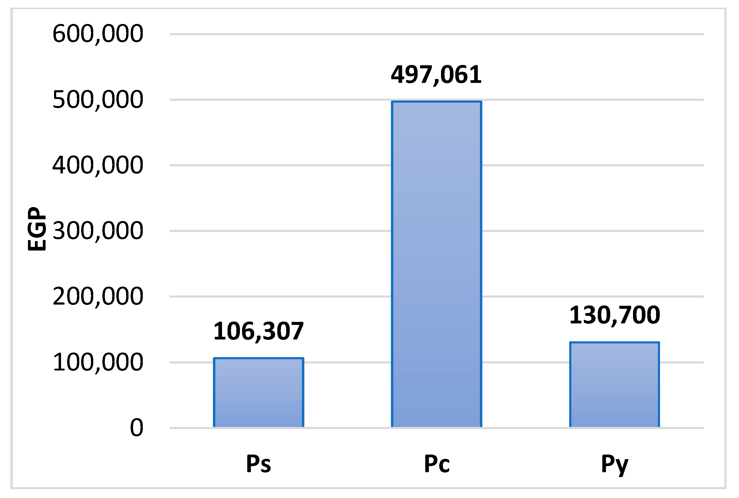
5.1. Complete Supply Chain Model Results

The model is solved using Gurobi Optimizer 10.0.2 on a laptop with Intel(R) Core (TM) i7-6500U CPU @ 2.50GHz and 16 GB RAM. The model results for the two time periods are presented in Figure 3 and Figure 4. These figures illustrate the optimum citrus supply chain (CSC) network and the transported quantities among supply chain echelons. The blue and orange arrows show the flow of citrus fruit and juice, respectively. The results indicate that only two suppliers (S1 and S2) are selected as they provide the lowest costs, and one processor (C1) is utilized due to its sufficient processing capacity.

Table 7. Complete citrus supply chain model results at t = 1 (quantities in kgs).

Source	Landfill (L)	Production	Inventory	Local Market (O)	Byproduct Market (B)
S1	L1: 213	-	-	O1: 426	-
S2	L1: 200	-	-	O2: 400	-
P1	L1: 471.54	14,161.8	-	O1: 1084.5	-
P2	L2: 284.3	8539.1	Fruit: 2070.3	O1: 1.14, O2: 653.9	-
C1	L1: 1965.8	54,200	-	-	B1: 27,100
X1	L1: 141.6	-	-	-	-
X2	L2: 64.68	-	-	-	-
R1	L1: 31.8	-	-	-	-
R2	L2: 32.7	-	Fruit: 120	-	-
R3	L2: 31.3	-	-	-	-
R4	L1: 31.4	-	-	-	-
Q1	L1: 20	-	-	-	-
Q2	L1: 19.2	-	-	-	-
Q3	L1: 19.6	-	-	-	-
Q4	L1: 18.18	-	-	-	-

and

Table 8. Complete citrus supply chain model results at t = 2 (quantities in kgs).

Source	Landfill (L)	Production	Inventory	Local Market (O)	Byproduct Market (B)
S1	L1: 213	-	-	O1: 426	-
S2	L1: 200	-	-	O2: 400	-
P1	L1: 606.8	18,223.5	-	O1: 1395.6	-
C1	L1: 2038.3	56,200	-	-	B1: 28,100
X1	L1: 173.6	-	-	-	-
X2	L2: 29.4	-	-	-	-
R1	L1: 31.3	-	-	-	-
R2	L2: 29.1	-	-	-	-
R3	L2: 31.7	-	-	-	-
R4	L1: 31.3	-	-	-	-
Q1	L1: 19.7	-	-	-	-
Q2	L1: 19.7	-	-	-	-
Q3	L1: 19.2	-	-	-	-
Q4	L1: 18.18	-	-	-	-

illustrate the quantities sent to landfills, production, and stored quantities, and the quantities transported to local markets and byproduct markets. According to the results, the complete supply chain profit is around EGP 4.48 million over the two weeks. Figure 5 displays the profit of each echelon in the supply chain, highlighting each echelon’s contribution to the overall profit.

5.2. Disruption Scenarios in Complete Supply Chain Model Results

5.2.1. Disruptions at Supplier

The results of Runs 1 and 2 indicate that disruptions at supplier 1 have a minimal impact on overall supply chain profit when compared to the supply chain profit before the occurrence of disruptions (base model), as shown in Figure 6. This is attributed to the resilience strategy of having multiple suppliers with sufficient capacity. Due to disruptions at supplier 1, the suppliers’ profits increase by around 1.3%, and this is because of the difference in the suppliers’ costs. Also, there is an increase in profits at the packhouse’s echelon, as one packhouse can satisfy the demand. On the contrary, the supplier disruption affects the processor’s echelon negatively, as the storage of juice is required; thus, the profits decrease. The fruit distributors and local retailers’ profits decreased slightly, due to changes in the transported quantities between echelons, whereas no change occurs at the juice distributors and the regional retailers. Run 3 results in an infeasible solution, underscoring the importance of having a multi-supplier strategy for meeting demands; therefore, this run is not presented in Figure 6.

As previously mentioned in Section 4.1, supply chain resilience is used as a performance measure to aid in determining the best resilience strategy. Supply chain resilience is calculated as the ratio between supply chain profit before and after the occurrence of disruption. The supply chain resilience for Runs 1 and 2 is close to 1 (0.99), confirming that having multiple suppliers is a sufficient strategy to achieve supply chain resilience, with no need for additional capacity under the given conditions.

5.2.2. Disruptions at Packhouse

Run 1 results demonstrate that a single packhouse suffices to meet the demand in the studied supply chain, with a decrease in supply chain profit of around EGP 10,500 over the two weeks when compared with the results of the base model, as shown in Figure 7. The same outputs are achieved in Run 2. In both runs, the profits at packhouse echelon decrease slightly due to the usage of packhouse 2, which leads to an increase in transportation costs, while the suppliers’ profits remain the same, since they send the same quantities to the working packhouse. The same happens with the juice distributors. The processors’ profits increase because they receive more units from suppliers directly at a cheaper price. There is a slight decrease in the fruit distributors’ profit because of the change in the supply chain configuration. The calculated supply chain resilience for both runs is 0.997. The aforementioned results prove that a 50% capacity increase in alternate packhouse (packhouse) 2 is not necessary.

5.2.3. Disruptions at Processor

Run 1 is infeasible as juice demand cannot be met with only one processor; therefore, this run is not presented in Figure 8. In Run 2, partial disruption of C1 results in a minor supply chain profit decrease of about EGP 9400, since the juice demand is still met with half of the processor’s capacity. In Run 3, the supply chain profit decreases by around EGP 18,000 when compared with the results of the base model, due to the difference in distances between the only functioning processor and other echelons, thus affecting the transportation costs. The supply chain profits in Runs 2 and 4 are the same. The calculated supply chain resilience for Run 3 is 0.99, highlighting the importance of having excess capacity when compared to Run 1’s resilience of 0. This underscores the necessity of fortifying the processor echelon in this supply chain. As same results are obtained in Runs 2 and 4, this indicates that there is no need for excess capacity during partial disruptions.

5.2.4. Disruptions at Outbound Logistics

Figure 9 shows that the supply chain profit significantly decreases in Run 1 because the products cannot reach the regional retailers, reducing the flow of fruits across all echelons and lowering profits at different echelons. The supply chain profit in Run 2 is slightly lower than the supply chain profit of the base model (before port disruptions) due to the increased transportation costs. The calculated resilience for Run 2 is 0.99, highlighting the importance of having an alternative route (port).

5.3. Case Study Model Results

The model outputs of the case study are displayed in Figure 10. According to the results, the third supplier is unnecessary in both periods, as only one supplier is sufficient per week.

Table 9. The case study model results at t = 1 (quantities in kgs).

Source	Landfill (L)	Production	Inventory	Local Market (O)	Byproduct Market (B)
S1	L1: 213	-	-	O2: 426	-
C1	L2: 1468.6	40,492.4	4246.2	-	B1: 20,246.2

and

Table 10. The case study model results at t = 2 (quantities in kgs).

Source	Landfill (L)	Production	Inventory	Local Market (O)	Byproduct Market (B)
S2	L1: 200	-	-	O2: 400	-
C1	L1: 1468.6	20,507.6	-	-	B1: 10,253.8

present the quantities sent to landfills, production, and stored quantities, and the quantities transported to local markets and byproduct markets. The supply chain profit for the case study is approximately EGP 73,400 over the two weeks, with the processor holding the largest share of the profits, as illustrated in Figure 11.

When running the case study model with full or partial disruption at the processor (Runs 1 and 2), an infeasible solution is obtained. This means that the supply chain is halted and there are lost sales. Run 3 also gives an infeasible solution, which represents having full disruptions at the processor and a backup facility with limited capacity. These runs are excluded from Figure 12. The supply chain profit in Run 4 is lower than the supply chain profit of the base model (before disruptions), due to the higher production cost of renting a backup production line. The calculated resilience of Run 4 is 0.9, highlighting the importance of having backup facility.

6. Conclusions and Implications

6.1. Conclusions

Due to increased volatility because of resource scarcity, disruptions, and climate variability, agri-food supply chains need to be resilient. As demand and supply are impacted by this volatility, there is therefore a necessity for resilient strategies. The primary goal of this study is to design a resilient and sustainable citrus supply chain (CSC) and its byproducts that can withstand disruptions while maintaining profitability. Supply chain sustainability is realized by reducing the waste sent to landfills and utilizing the generated processing waste. This study fills a gap in the literature by studying resilience strategies to build a resilient CSC and designing a complete citrus supply chain, from farm to retailer, which includes the production of citrus fruit and juice and deals with citrus waste simultaneously. This study answers the following questions: (1) What is the optimum citrus supply chain network design that maximizes the supply chain? (2) What resilient strategy is advised to be applied in the supply chain network in the event that suppliers, packhouses, processors, and outbound logistics experience disruptions?

A multi-period mixed-integer linear programming model is developed for designing a resilient sustainable CSC, encompassing both fruits and juice. The model maximizes the supply chain profit and determines the operational status of facilities, transportation quantities between echelons, processing quantities at packhouses and processors, and inventory levels at each facility. The model is solved using Gurobi optimization software 10.0.2.

A complete CSC scenario in Egypt, including citrus fruit and juice, is developed to justify the applicability of the proposed model. The input data are collected from CSC stakeholders in Egypt. By solving the model, the best supply chain configuration which maximizes the supply chain profit is achieved. Various disruption scenarios are analyzed to identify the most effective strategy to face disruptions occurring at different echelons, highlighting the importance of supply chain resilience. Key strategies such as multiple suppliers, backup processor capacity, and alternative logistics routes help in attaining supply chain resilience.

An actual Egyptian organic orange juice supply chain of a company that supplies both local and regional customers is optimized using the developed model, demonstrating the model’s efficacy in real-world applications. Disruption scenarios at the processor are examined for this supply chain and the results highlight the importance of having a backup facility.

6.2. Managerial Implications

Firstly, the proposed model could help managers and decision makers in designing a complete CSC network, encompassing the entire supply chain from farm to fork that includes citrus fruit, juice, and waste. It helps in maximizing supply chain profit and determining the operational status of each facility in the network, transported quantities between all echelons, processing quantities at packhouses and processors, and determining inventory levels at each facility. It incorporates constraints related to production capacities, inventory capacities, the flow balance of fruits and juice, demand satisfaction, waste quantities, and the quality of non-conforming fruits. The proposed model could be modified to fit other agri-food products, which could have different characteristics and perishability levels.

Secondly, this study introduces sustainability in the developed CSC network through maximizing supply chain profit, reducing waste sent to landfills, and valorizing CPW by selling it to intermediaries or processors working with CPW.

Finally, this study provides practical insights and recommendations for building a resilient CSC. The following resilience strategies are recommended based on the assessed disruption scenarios:

• A multi-supplier strategy aids in achieving supply chain resilience in the event of complete disruptions in one of the suppliers.
• Having more than one packhouse could be sufficient for being resilient without increasing the capacities of existing packhouses in the case of complete disruption in one of the packhouses.
• In case one of the processors completely fails, it might be essential to increase the capacity of the operational processors or have a backup facility with enough capacity.
• It might be necessary to consider an alternative port in case of disruptions in present ports.

6.3. Future Work

There are limitations during this study that might stimulate future work. Firstly, the large amount of input data required for running the model poses a significant burden in terms of time and effort in data preprocessing, especially with the increase in the number of periods to be included in the model. Therefore, finding a suitable approach to facilitate data entry is required. Secondly, the citrus byproduct market can be explored in greater detail by categorizing the different byproduct types and incorporating their supply chains into the developed model. Thirdly, the proposed model can be extended to be multi-objective, for example, by considering the minimization of CO₂ emissions. Moreover, the transportation decisions on vehicle types and capacities can be included in the model. Finally, the model developed can be modified to consider uncertainty, and a sensitivity analysis of key parameters could be conducted.

References

1. Sherman, E. 94% of the Fortune 1000 are Seeing Coronavirus Supply Chain Disruptions: Report. 2020. Available online: https://fortune.com/2020/02/21/fortune-1000-coronavirus-china-supply-chain-impact/ (accessed on 10 April 2025).
2. Emenike, S.N.; Falcone, G. A review on energy supply chain resilience through optimization. Renew. Sustain. Energy Rev. 2020, 134, 110088. [Google Scholar] [CrossRef]
3. Mariana, O.S.; Alzate, C.; Ariel, C. Comparative environmental life cycle assessment of orange peel waste in present productive chains. J. Clean. Prod. 2021, 322, 128814. [Google Scholar] [CrossRef]
4. Knoema. Agriculture Crops Production Citrus Fruit Production. 2023. Available online: https://knoema.com/atlas/World/topics/Agriculture/Crops-Production-Quantity-tonnes/Citrus-fruit-production#:~:text=Citrus%20fruit%20production%20of%20World,by%20our%20digital%20data%20assistant (accessed on 10 April 2025).
5. FAO. FAO Stat: Food and Agriculture Data. 2025. Available online: https://www.fao.org/faostat/en/#data/TCL (accessed on 10 April 2025).
6. Beshara, S.; Kassem, A.; Fors, H.; Harraz, N. A Comprehensive Review and Mapping Citrus Supply Chains from a Sustainability Perspective across the European Union, Middle East, and Africa. Sustainability 2024, 16, 8582. [Google Scholar] [CrossRef]
7. Valverde, C. Report Name: Citrus Annual; EU Citrus Annual Report; USDA: Washington, DC, USA, 2021; pp. 1–20. [Google Scholar]
8. USDA/FAS. Citrus: World Markets and Trade. In U.S. Production and Exports Forecast Down Despite Global Gains; United States Department of Agriculture, Foreign Agricultural Service: Washington, DC, USA, 2021; pp. 1–13. [Google Scholar]
9. Beshara, S.; Fors, H.; Harraz, N. Designing Supply Chain to Hedge Against Disruptions: A Review of Literature in General and Agro Food Supply Chains; IEOM Society International: Southfield, MI, USA, 2022; pp. 135–146. [Google Scholar] [CrossRef]
10. Li, Z.; Zhao, P.; Han, X. Agri-food supply chain network disruption propagation and recovery based on cascading failure. Phys. A Stat. Mech. Its Appl. 2022, 589, 126611. [Google Scholar] [CrossRef]
11. Zhao, G.; Liu, S.; Lopez, C.; Chen, H.; Lu, H.; Mangla, S.K.; Elgueta, S. Risk analysis of the agri-food supply chain: A multi-method approach. Int. J. Prod. Res. 2020, 58, 4851–4876. [Google Scholar] [CrossRef]
12. Behzadi, G.; O’Sullivan, M.J.; Olsen, T.L.; Zhang, A. Allocation flexibility for agribusiness supply chains under market demand disruption. Int. J. Prod. Res. 2018, 56, 3524–3546. [Google Scholar] [CrossRef]
13. Gholami-Zanjani, S.M.; Jabalameli, M.S.; Klibi, W.; Pishvaee, M.S. A robust location-inventory model for food supply chains operating under disruptions with ripple effects. Int. J. Prod. Res. 2021, 59, 301–324. [Google Scholar] [CrossRef]
14. Esteso, A.; Alemany, M.M.E.; Ortiz, A. Conceptual framework for designing agri-food supply chains under uncertainty by mathematical programming models. Int. J. Prod. Res. 2018, 56, 4418–4446. [Google Scholar] [CrossRef]
15. Stone, J.; Rahimifard, S. Resilience in agri-food supply chains: A critical analysis of the literature and synthesis of a novel framework. Supply Chain Manag. 2018, 23, 207–238. [Google Scholar] [CrossRef]
16. Ravulakollu, A.K.; Urciuoli, L.; Rukanova, B.; Tan, Y.H.; Hakvoort, R.A. Risk based framework for assessing resilience in a complex multi-actor supply chain domain. Supply Chain Forum 2018, 19, 266–281. [Google Scholar] [CrossRef]
17. Bottani, E.; Murino, T.; Schiavo, M.; Akkerman, R. Resilient food supply chain design: Modelling framework and metaheuristic solution approach. Comput. Ind. Eng. 2019, 135, 177–198. [Google Scholar] [CrossRef]
18. Liao, Y.; Kaviyani-Charati, M.; Hajiaghaei-Keshteli, M.; Diabat, A. Designing a closed-loop supply chain network for citrus fruits crates considering environmental and economic issues. J. Manuf. Syst. 2020, 55, 199–220. [Google Scholar] [CrossRef]
19. Behzadi, G.; O’Sullivan, M.J.; Olsen, T.L. On metrics for supply chain resilience. Eur. J. Oper. Res. 2020, 287, 145–158. [Google Scholar] [CrossRef]
20. Mohib, A.M.N.; Deif, A.M. Supply chain multi-state risk assessment using universal generating function. Prod. Plan. Control 2020, 31, 699–708. [Google Scholar] [CrossRef]
21. Sharma, P.; Vishvakarma, R.; Gautam, K.; Vimal, A.; Kumar Gaur, V.; Farooqui, A.; Varjani, S.; Younis, K. Valorization of citrus peel waste for the sustainable production of value-added products. Bioresour. Technol. 2022, 351, 127064. [Google Scholar] [CrossRef]
22. Gholami-Zanjani, S.M.; Klibi, W.; Jabalameli, M.S.; Pishvaee, M.S. The design of resilient food supply chain networks prone to epidemic disruptions. Int. J. Prod. Econ. 2021, 233, 108001. [Google Scholar] [CrossRef]
23. Abu Hatab, A.; Lagerkvist, C.J.; Esmat, A. Risk perception and determinants in small- and medium-sized agri-food enterprises amidst the COVID-19 pandemic: Evidence from Egypt. Agribusiness 2021, 37, 187–212. [Google Scholar] [CrossRef]
24. Ali, A.; Xia, C.; Ismaiel, M.; Ouattara, N.B.; Mahmood, I.; Anshiso, D. Analysis of determinants to mitigate food losses and waste in the developing countries: Empirical evidence from Egypt. Mitig. Adapt. Strateg. Glob. Change 2021, 26, 23. [Google Scholar] [CrossRef]
25. Zhao, G.; Vazquez-Noguerol, M.; Liu, S.; Prado-Prado, J.C. Agri-food supply chain resilience strategies for preparing, responding, recovering, and adapting in relation to unexpected crisis: A cross-country comparative analysis from the COVID-19 pandemic. J. Bus. Logist. 2023, 45, e12361. [Google Scholar] [CrossRef]
26. Li, Z.; Zhang, C. Designing a two-stage model for the resilient agri-food supply chain network under dynamic competition. Br. Food J. 2024, 126, 662–681. [Google Scholar] [CrossRef]
27. Miranda-Ackerman, M.A.; Azzaro-Pantel, C.; Aguilar-Lasserre, A.A. A green supply chain network design framework for the processed food industry: Application to the orange juice agrofood cluster. Comput. Ind. Eng. 2017, 109, 369–389. [Google Scholar] [CrossRef]
28. Peña-Orozco, D.L.; Gonzalez-Feliu, J.; Salazar-Aguirre, L.T.; Arenas-Ruiz, M.A. Sustainability Fruit Supply Chain Design in the Context of Decentralized Smallholders: Modelling Framework and Sensitivity Analysis. LOGI—Sci. J. Transp. Logist. 2023, 14, 43–54. [Google Scholar] [CrossRef]
29. Darley-Waddilove, J.I. Allocating Commodity Volumes in the Citrus Export Cold Chain. Master’s Thesis, Stellenbosch University, Stellenbosch, South Africa, 2021. [Google Scholar]
30. Cheraghalipour, A.; Paydar, M.M.; Hajiaghaei-Keshteli, M. A bi-objective optimization for citrus closed-loop supply chain using Pareto-based algorithms. Appl. Soft Comput. J. 2018, 69, 33–59. [Google Scholar] [CrossRef]
31. Imbachi, C.G.A.; Larrahondo, A.F.C.; Orozco, D.L.P.; Cadavid, L.R.; Bastidas, J.J.B. Design of an inventory management system in an agricultural supply chain considering the deterioration of the product: The case of small citrus producers in a developing country. J. Appl. Eng. Sci. 2018, 16, 523–537. [Google Scholar] [CrossRef]
32. Roghanian, E.; Cheraghalipour, A. Addressing a set of meta-heuristics to solve a multi-objective model for closed-loop citrus supply chain considering CO2 emissions. J. Clean. Prod. 2019, 239, 118081. [Google Scholar] [CrossRef]
33. Aslan, H.; Zereyak, E.; Rad, S.T. Modelling of Citrus Production and Export Process: Eastern Mediterrenean Region of Turkey. Karadeniz Uluslararası Bilimsel Dergi 2020, 48, 169–187. [Google Scholar] [CrossRef]
34. Sahebjamnia, N.; Goodarzian, F.; Hajiaghaei-Keshteli, M. Optimization of multi-period three-echelon citrus supply chain problem. J. Optim. Ind. Eng. 2020, 13, 39–53. [Google Scholar] [CrossRef]
35. Goodarzian, F.; Fakhrzad, M.B. A New Multi-Objective Mathematical Model for A Citrus Supply Chain Network Design: Metaheuristic Algorithms. J. Optim. Ind. Eng. 2021, 14, 127–144. [Google Scholar] [CrossRef]
36. Peña Orozco, D.L.; Gonzalez-Feliu, J.; Rivera, L.; Mejía Ramirez, C.A. Integration maturity analysis for a small citrus producers’ supply chain in a developing country. Bus. Process Manag. J. 2021, 27, 836–867. [Google Scholar] [CrossRef]
37. Güner, G.G.; Utku, D.H. An Optimization Approach for a Fresh Food Supply Chain: An Application for the Orange Supply Chain Design in Turkey. Düzce Üniversitesi Bilim Ve Teknol. Derg. 2021, 9, 1563. [Google Scholar] [CrossRef]
38. Alzubi, E.; Noche, B. A multi-objective model to find the sustainable location for citrus hub. Sustainability 2022, 14, 4463. [Google Scholar] [CrossRef]
39. Alzubi, E.; Shbikat, N.; Noche, B. A system dynamics model to improving sustainable performance of the citrus farmers in Jordan Valley. Clean. Prod. Lett. 2023, 4, 100034. [Google Scholar] [CrossRef]
40. Goodarzian, F.; Ghasemi, P.; Santibanez Gonzalez, E.D.; Tirkolaee, E.B. A sustainable-circular citrus closed-loop supply chain configuration: Pareto-based algorithms. J. Environ. Manag. 2023, 328, 116892. [Google Scholar] [CrossRef] [PubMed]
41. Paredes-Rodríguez, A.M.; Osorio-Gómez, J.C.; Orejuela-Cabrera, J.P. Dynamic evaluation of distribution channels in a fresh food supply chain from a sustainability and resilience approach. Alex. Eng. J. 2024, 106, 42–51. [Google Scholar] [CrossRef]
42. Goodarzian, F.; Kumar, V.; Ghasemi, P. Investigating a citrus fruit supply chain network considering CO2 emissions using meta-heuristic algorithms. Ann. Oper. Res. 2024, 332, 1301. [Google Scholar] [CrossRef]
43. Zhao, S.; You, F. Resilient supply chain design and operations with decision-dependent uncertainty using a data-driven robust optimization approach. AIChE J. 2019, 65, 1006–1021. [Google Scholar] [CrossRef]
Figure 1. Citrus supply chain network design.
Logistics 09 00066 g001
Figure 2. Supply chain of the case study.
Logistics 09 00066 g002
Figure 3. The complete citrus supply chain network at t = 1.
Logistics 09 00066 g003
Figure 4. The complete citrus supply chain network at t = 2.
Logistics 09 00066 g004
Figure 5. Profit of each echelon in the complete citrus supply chain.
Logistics 09 00066 g005
Figure 6. Optimal objective function value of runs related to supplier disruptions.
Logistics 09 00066 g006
Figure 7. Optimal objective function value of runs related to packhouse disruptions.
Logistics 09 00066 g007
Figure 8. Optimal objective function value of runs related to processor disruptions.
Logistics 09 00066 g008
Figure 9. Optimal objective function value of runs related to outbound logistics disruptions.
Logistics 09 00066 g009
Figure 10. The case study model outputs at t = 1 and 2.
Logistics 09 00066 g010
Figure 11. Profit of each echelon in the case study supply chain.
Logistics 09 00066 g011
Figure 12. Optimal objective function value of runs related to processor disruptions.
Logistics 09 00066 g012