
The Gamma Distribution and Inventory Control: Disruptive Lead Times Under Conventional and Nonclassical Conditions

Abstract
1. Introduction
2. Literature Review
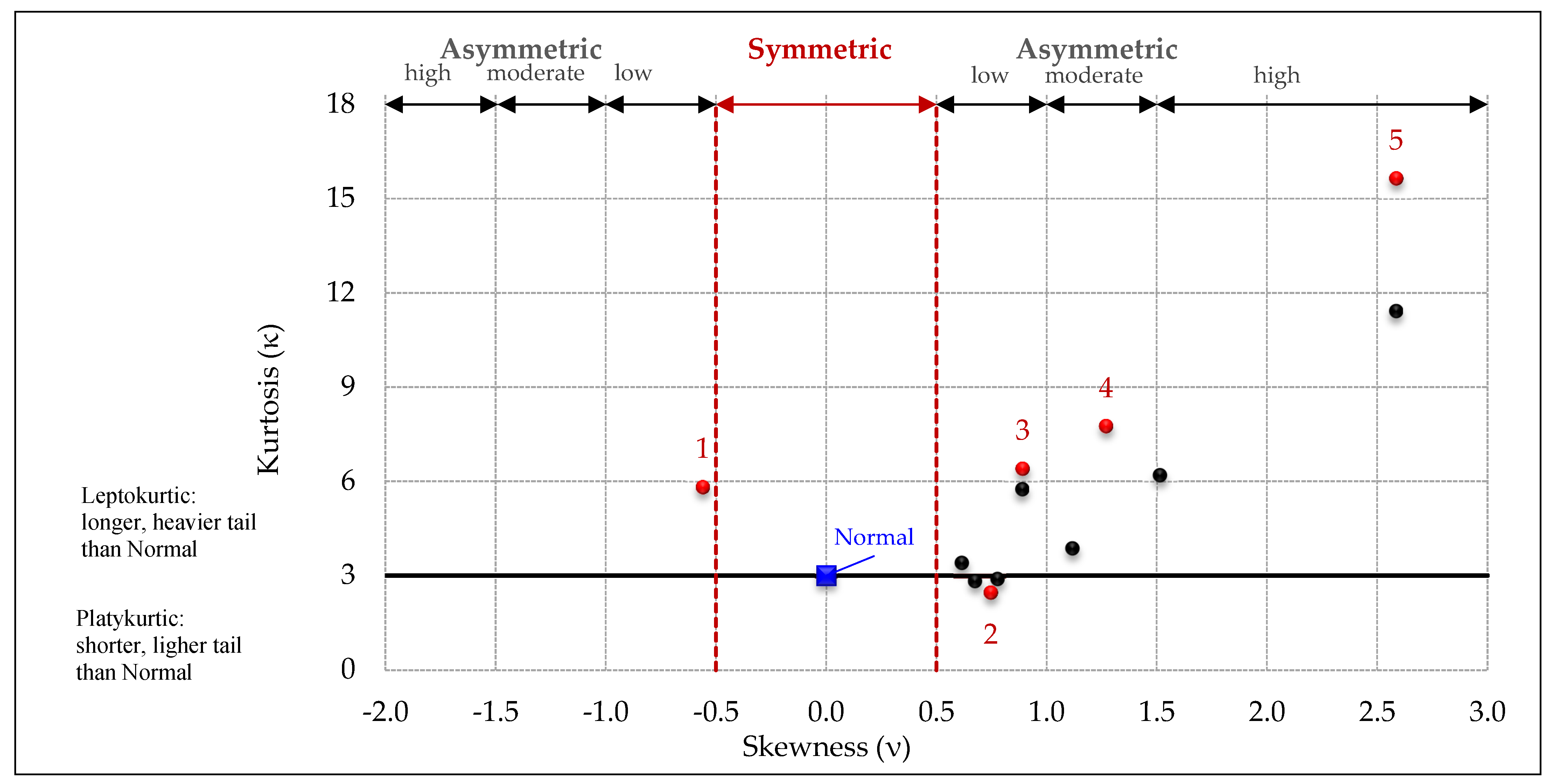
2.1. Higher Moments
2.2. Accuracy Constructs
3. Methods
3.1. Business Setting
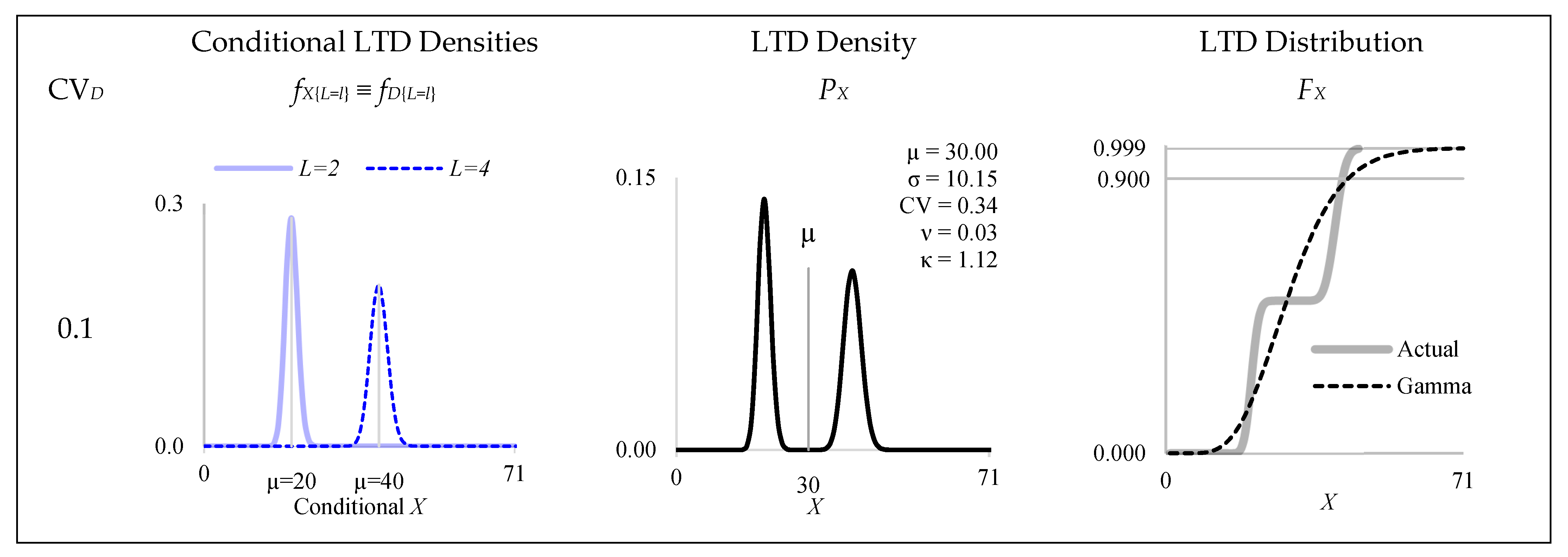
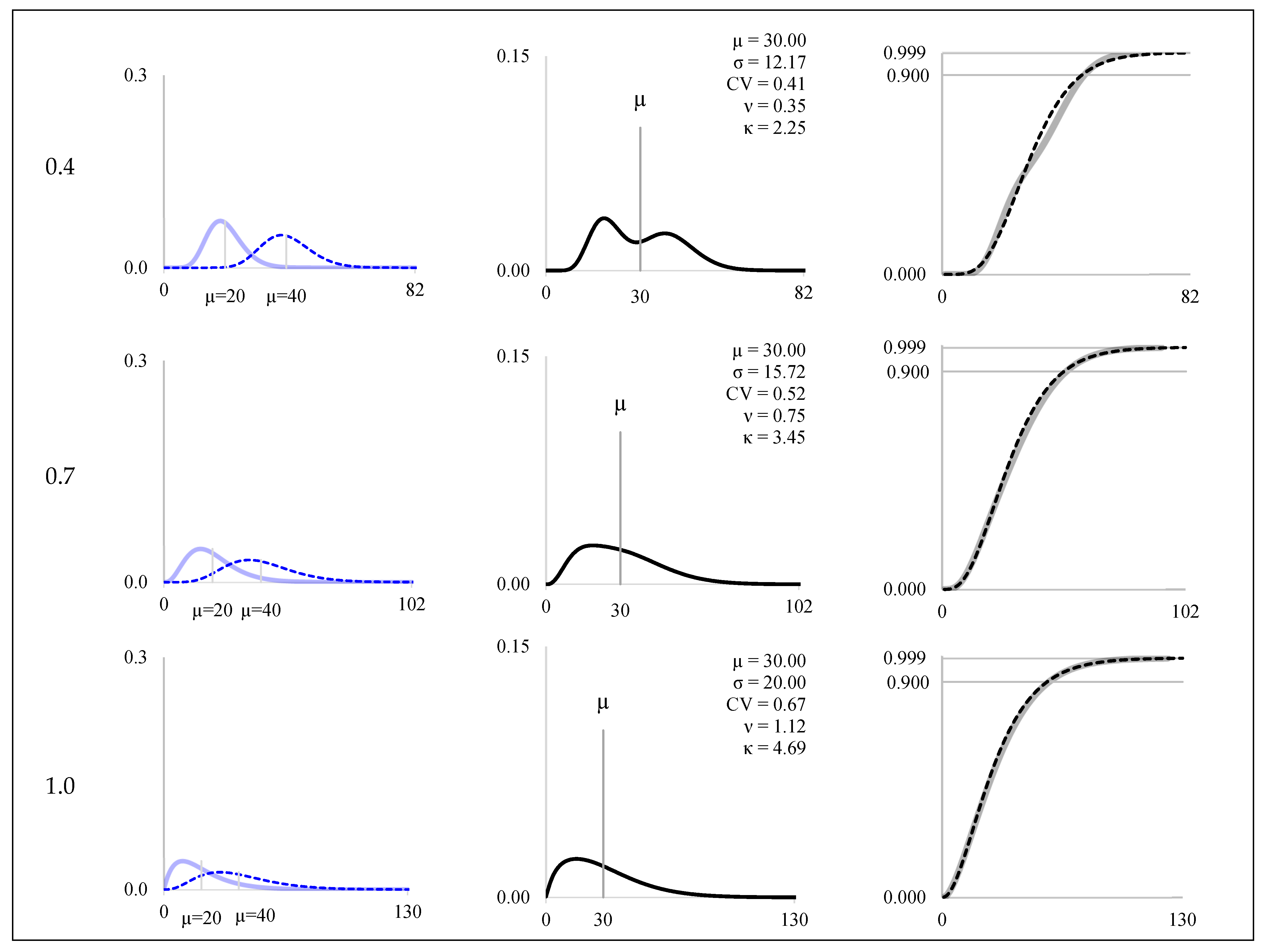
3.1.1. Demand
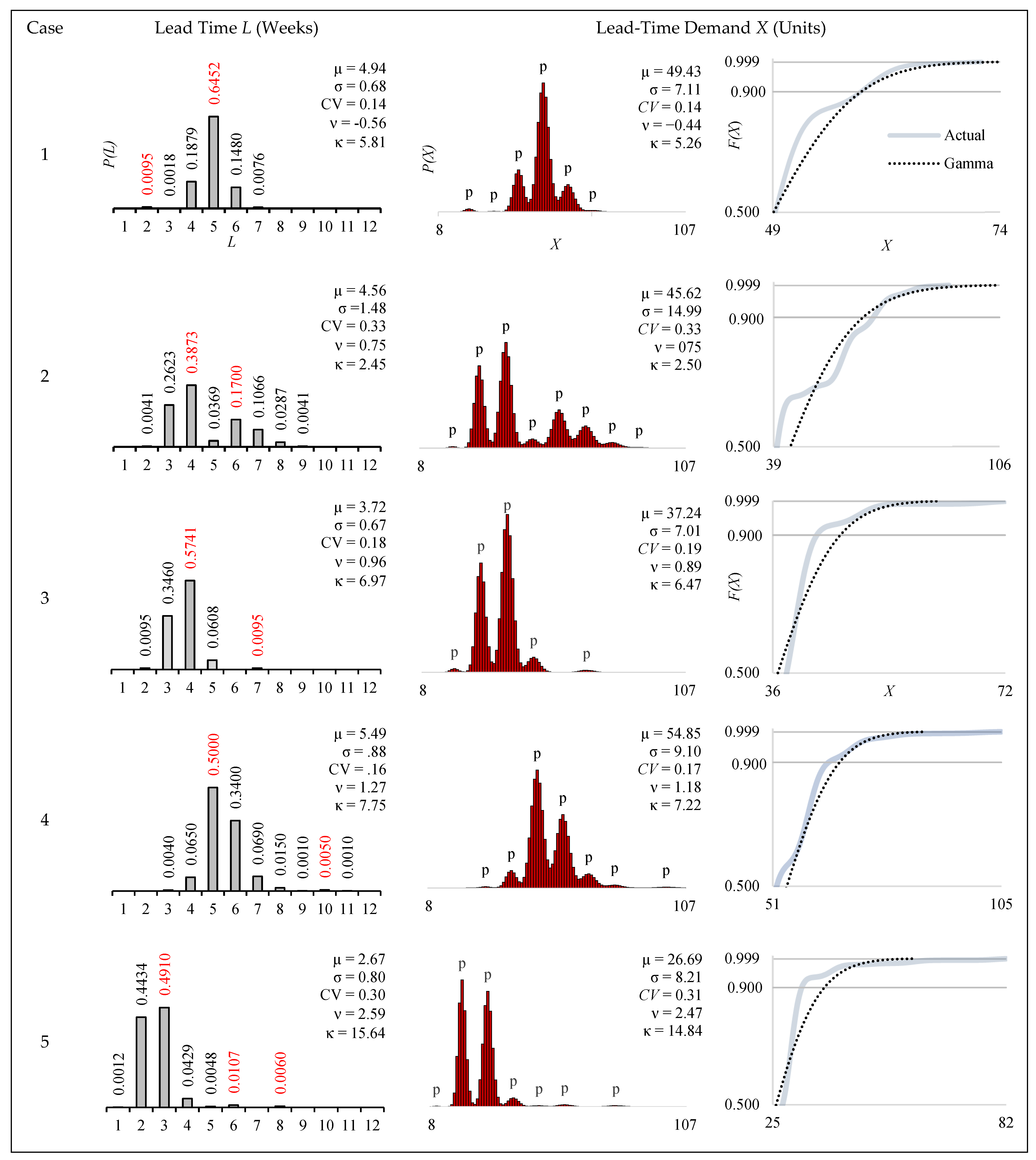
3.1.2. Lead Time
3.2. Conventional LTD Scenario (X)
3.3. Numerical Experiments
3.3.1. Dependent Variables
3.3.2. Independent Variables
Setting Variables
Experimental Variables
System Variables
3.4. Nonclassical LTD Scenarios
3.4.1. Serial Correlation (U)
3.4.2. Random Order Crossover (Y, W)
4. Results
4.1. One Open Order (X, U)
4.2. Multiple Open Orders (U, W)
5. Discussion
5.1. External Validation
5.2. Propositions
6. Conclusions
Supplementary Materials
Funding
Data Availability Statement
Acknowledgments
Conflicts of Interest
Abbreviations
| AHC | Annual holding cost |
| AOC | Annual order cost |
| ASC | Annual shortage cost |
| ATC | Annual total cost |
| CR | Critical ratio |
| CSC | Cycle stock holding cost (annual) |
| CV | Coefficient of variation |
| ELT | Effective lead time |
| LTD | Lead-time demand |
| ROC | Random order crossover |
| SSC | Safety stock holding cost (annual) |
References
- Burgin, T.A. The gamma distribution and inventory control. Oper. Res. Q. (1970–1977) 1975, 26, 507–525. [Google Scholar] [CrossRef]
- Chopra, S.; Reinhardt, G.; Dada, M. The effect of lead time uncertainty on safety stocks. Decis. Sci. 2004, 35, 1–24. [Google Scholar] [CrossRef]
- Cobb, B.R.; Johnson, A.W.; Rumí, R.; Salmerón, A. Accurate lead time demand modelling and optimal inventory policies in continuous review systems. Int. J. Prod. Econ. 2015, 163, 124–136. [Google Scholar] [CrossRef]
- Disney, S.M.; Maltz, A.; Wang, X.; Warburton, R.H. Inventory management for stochastic lead times with order crossovers. Eur. J. Oper. Res. 2016, 248, 473–486. [Google Scholar] [CrossRef]
- Eppen, G.D.; Martin, R.K. Determining safety stock in the presence of stochastic lead time and demand. Manag. Sci. 1988, 34, 1380–1390. [Google Scholar] [CrossRef]
- Lau, H.; Lau, A. A simple cost minimization procedure for the (Q,R) inventory model: Development and evaluation. IIE Trans. 1993, 25, 45–52. [Google Scholar] [CrossRef]
- Saldanha, J.P. Estimating the reorder point for a fill-rate target under a continuous review policy in the presence of non-standard lead-time demand distributions. Transp. Res. Part E Logist. Transp. Rev. 2022, 164, 102766. [Google Scholar] [CrossRef]
- Saldanha, J.P.; Price, B.S.; Thomas, D.J. A nonparametric approach for setting safety stock levels. Prod. Oper. Manag. 2023, 32, 1150–1168. [Google Scholar] [CrossRef]
- UNCTAD. Global Report on Blockchain and its Implications on Trade Facilitation Performance. 2023. Available online: https://unctad.org/publication/global-report-blockchain-and-its-implications-trade-facilitation-performance (accessed on 26 February 2025).
- Fetter, R.; Dalleck, W. Decision Models for Inventory Management. Available online: https://catalogue.nla.gov.au/Record/754678 (accessed on 26 February 2025).
- Saoud, P.; Kourentzes, N.; Boylan, J. Approximations for lead time variance: A forecasting and inventory evaluation. Omega 2022, 110, 102614. [Google Scholar] [CrossRef]
- Hadley, G.; Whitin, T.M. Analysis of Inventory Systems; Prentice-Hall: Englewood Cliffs, NJ, USA, 1963. [Google Scholar]
- Naddor, E. Note—Sensitivity to distributions in inventory systems. Manag. Sci. 1978, 24, 1769–1772. [Google Scholar] [CrossRef]
- Kaki, A.; Salo, A.; Talluri, S. Impact of the shape of the demand distribution in decision models for operations management. Comput. Ind. 2013, 64, 765–775. [Google Scholar] [CrossRef]
- Riezbos, J. Inventory order crossovers. Int. J. Prod. Econ. 2006, 104, 666–675. [Google Scholar] [CrossRef]
- Leachman, R.C. Final Report–Port and Modal Elasticity Study. In Proceedings of the Southern California Association of Governments by Leachman Associates LLC 2005, Los Angeles, CA, USA, 8 September 2005. [Google Scholar]
- Fortuin, L. Five popular probability density functions: A comparison in the field of stock-control models. J. Oper. Res. Soc. 1980, 31, 937–942. [Google Scholar] [CrossRef]
- Tadikamalla, P.R. A comparison of several approximations to the lead time demand distribution. Omega 1984, 12, 575–581. [Google Scholar] [CrossRef]
- Heuts, R.; Lieshout, J.V.; Baken, K. An inventory model: What is the influence of the shape of the lead time demand distribution? Z. FüR Oper. Res. 1986, 30, B1–B14. [Google Scholar] [CrossRef]
- Bartezzaghi, E.; Verganti, R.; Zotteri, G. Measuring the impact of asymmetric demand distributions on inventories. Int. J. Prod. Econ. 1999, 60–61, 395–404. [Google Scholar] [CrossRef]
- Rossetti, M.D.; Unlu, Y. Evaluating the robustness of lead-time demand models. Int. J. Prod. Econ. 2011, 134, 159–176. [Google Scholar] [CrossRef]
- Tyworth, J.E.; O’Neill, L. Robustness of the normal approximation of lead-time demand in a distribution setting. Nav. Res. Logist. 1997, 42, 165–186. [Google Scholar] [CrossRef]
- Cobb, B.R.; Rumí, R.; Salmerón, A. Inventory management with log-normal demand per unit time. Comput. Oper. Res. 2013, 40, 1842–1852. [Google Scholar] [CrossRef]
- Cobb, B.R. Mixture distributions for modelling demand during lead time. J. Oper. Res. Soc. 2013, 64, 217–228. [Google Scholar] [CrossRef]
- Tyworth, J.; Guo, Y.; Ganeshan, R. Inventory control under gamma demand and random lead time. J. Bus. Logist. 1996, 17, 291–304. [Google Scholar]
- Fisher, M.L. What Is the Right Supply Chain for Your Product? Harvard Business Review, March–April 1977, pp. 105–116. Available online: https://hbr.org/1997/03/what-is-the-right-supply-chain-for-your-product (accessed on 26 February 2025).
- Harris, G.; Farrington, P. An exploration of Fisher’s framework for the alignment of supply chain strategy with product characteristics. Eng. Manag. J. 2015, 22, 31–43. [Google Scholar] [CrossRef]
- Chen, C.; Thomas, D.J. Inventory allocation in the presence of service-level agreements. Prod. Oper. Manag. 2018, 27, 553–577. [Google Scholar] [CrossRef]
- Tyworth, J.E. A note on lead-time paradoxes and a tale of competing prescriptions. Transp. Res. Part E Logist. Transp. Rev. 2018, 109, 139–150. [Google Scholar] [CrossRef]
- Vernimmen, B.; Dullaert, W.; Willeme, P.; Witlox, F. Using the inventory-theoretic framework to determine cost-minimizing supply strategies in a stochastic setting. Int. J. Prod. Econ. 2008, 115, 248–259. [Google Scholar] [CrossRef]
- Hayya, J.C.; Bagchi, U.; Kim, J.G.; Sun, D. On static stochastic order crossover. Int. J. Prod. Econ. 2008, 114, 404–413. [Google Scholar] [CrossRef]
- Chatfield, D.C.; Pritchard, A.M. Crossover aware base stock decisions for service-driven systems. Transp. Res. Part E 2018, 114, 312–330. [Google Scholar] [CrossRef]
- Das, L.; Kalkanci, B.; Caplice, C. Impact of bimodal and lognormal distributions in ocean transit time on logistics costs. Transp. Res. Rec. 2014, 2049, 63–73. [Google Scholar] [CrossRef]
- Bischak, D.P.; Robb, D.J.; Silver, E.A.; Blackburn, J.D. Analysis and management of periodic review, order-up-to level inventory systems with order crossover. Prod. Oper. Manag. 2014, 23, 762–772. [Google Scholar] [CrossRef]
- Silver, E.A.; Robb, D.J. Some insights regarding the optimal reorder period in periodic review inventory systems. Int. J. Prod. Econ. 2008, 112, 354–366. [Google Scholar] [CrossRef]
- Fang, X.; Zhang, C.; Robb, D.J.; Blackburn, J.D. Decision support for lead time demand variability reduction. Omega 2013, 41, 390–396. [Google Scholar] [CrossRef]
- Teunter, R.H.; Babai, M.Z.; Syntetos, A.A. ABC classification: Service levels inventory costs. Prod. Oper. Manag. 2010, 19, 343–352. [Google Scholar] [CrossRef]
- Kapuscinski, R.; Zhang, R.Q.; Carbonneau, P.; Moore, R.; Reeves, B. Inventory decisions in Dell’s supply chain. Interfaces 2004, 34, 191–205. [Google Scholar] [CrossRef]
- Yang, L.; Liu, K.; Zhang, J.; Zelbst, P. Inventory management with actual palletized transportation costs and lost sales. Transp. Res. Part E Logist. Transp. Rev. 2024, 184, 103462. [Google Scholar] [CrossRef]
- Holmes, T.; Singer, E. Indivisibilities in Distribution; Working Paper 24525; National Bureau of Economic Research: Cambridge, MA, USA, 2018; Available online: http://www.nber.org/papers/w24525 (accessed on 26 February 2025). [CrossRef]
- Jain, N.; Girotra, K.; Natesan, S. Managing global sourcing: Inventory performance. Manag. Sci. 2014, 60, 1202–1222. [Google Scholar] [CrossRef]
- Arsyida, T.T. Trade Compliance Cost Model in the International Supply Chain. Master’s Thesis, Delft University of Technology, Delft, The Netherlands, 2017. Available online: http://resolver.tudelft.nl/uuid:94a9226d-362d-4bf7-a97f-cc908289ff6e (accessed on 26 February 2025).
- Grainger, A. Trade and customs compliance costs at ports. Marit. Econ. Logist. 2014, 16, 467–483. [Google Scholar] [CrossRef]
- Kropf, A.; Sauré, P. Fixed costs per shipment. J. Int. Econ. 2014, 92, 166–184. [Google Scholar] [CrossRef]
- Tempelmeier, H. Inventory Management in Supply Networks, 2nd ed.; The University of Cologne: Cologne, Germany, 2011. [Google Scholar]
- Silver, E.; Pyke, D.; Thomas, D. Inventory and Production Management in Supply Chains, 4th ed.; Wiley: New York, NY, USA, 2017. [Google Scholar]
- Fenton, L. The sum of log-normal probability distributions in scatter transmission systems. IEEE Trans. Commun. 1960, 8, 57–67. [Google Scholar] [CrossRef]
- Keaton, M. Using the gamma distribution to model demand when lead time is random. J. Bus. Logist. 1995, 16, 107–132. [Google Scholar]
- Caplice, C.; Kalkanci, B. Ocean Transportation Reliability: Myths, Realities, and Impacts. Webinar Slides, MIT, MIT Center for Transportation Logistics, 2011, 2012. Available online: https://ctl.mit.edu/sites/default/files/Ocean_Transportation_Reliability_Webinar.pdf (accessed on 26 February 2025).
- Caplice, C.; Kalkanci, B. Global Supply Chain Variability. In Proceedings of the CSCMP Annual Global Conference, Atlanta, GA, USA, 30 September–3 October 2012. [Google Scholar]
- Caplice, C.; Kalkanci, B. Managing Global Supply Chains: Building End-to-End Reliability; MIT, Center for Transportation Logistics: Cambridge, MA, USA, 2012; Available online: https://freightlab.mit.edu/wp-content/uploads/2020/02/2012-MIT-Freightlab-GlobalOceanTransport_RoundtableReport_Final.pdf (accessed on 26 February 2025).
- Das, L. The Impact of Bimodal Distribution in Ocean Transit Time on Logistics Costs: An Empirical and Theoretical Analysis. Master’s Thesis, Massachusetts Institute of Technology, Cambridge, MA, USA, June 2013. [Google Scholar]
- Lau, H.; Lau, A. Nonrobustness of the normal approximation of lead-time demand in a (Q, R) system. Nav. Res. Logist. 2003, 50, 149–166. [Google Scholar] [CrossRef]
- Brown, S. Measures of Shape: Skewness and Kurtosis. Available online: https://brownmath.com/stat/shape.htm (accessed on 26 February 2025).
- Syntetos, A.A.; Boylan, J.E.; Croston, J.D. On the categorization of demand patterns. J. Oper. Res. Soc. 2005, 56, 495–503. [Google Scholar] [CrossRef]
- Babai, M.Z.; Dai, Y.; Li, Q.; Syntetos, A.; Wang, X. Forecasting of lead-time demand variance: Implications for safety stock calculations. Eur. J. Oper. Res. 2022, 296, 846–861. [Google Scholar] [CrossRef]
- Prak, D.; Tuenter, R.; Syntetos, A. On the calculation of safety stocks when demand is forecasted. Eur. J. Oper. Res. 2017, 256, 454–461. [Google Scholar] [CrossRef]
- Wensing, T.; Kuhn, H. Analysis of production and inventory systems when orders may cross over. Ann. Oper. Res. 2015, 231, 265–281. [Google Scholar] [CrossRef]
- Saldanha, J.P.; Swan, P. Order crossover research: A 60-year retrospective to highlight future research opportunities. Transp. J. 2017, 50, 227–262. [Google Scholar] [CrossRef]
- Robinson, L.W.; Bradley, J.R.; Thomas, L.J. The impact of lead-time variability on inventory systems. Manuf. Serv. Oper. Manag. 2001, 3, 175–188. [Google Scholar] [CrossRef]
- Anderson, E.T.; Fitzsimons, G.J.; Simester, D. Measuring and mitigating the costs of stockouts. Manag. Sci. 2006, 52, 1751–1763. [Google Scholar] [CrossRef]
- F. Curtis Barry and Company. Understanding the True Cost of a Backorder in Your Operations. 2025. Available online: https://www.fcbco.com/blog/the-true-cost-of-a-back-order (accessed on 26 February 2025).
- Kumar, P.; Choubey, D.; Amosu, O.; Ogunsuji, Y. AI-enhanced inventory and demand forecasting: Using AI to optimize inventory management and predict customer demand. World J. Adv. Res. Rev. 2024, 23, 1931–1944. [Google Scholar] [CrossRef]
- Rashid, A.; Rasheed, R.; Ngah, A.; Amirah, N.A. Unleashing the power of cloud adoption and artificial intelligence in optimizing resilience and sustainable manufacturing supply chain in the USA. J. Manuf. Technol. Manag. 2024, 35, 1329–1353. [Google Scholar] [CrossRef]


| Normal | Gamma | ||
|---|---|---|---|
| Source | Data | Source | Data |
| Das et al. [33] | Retail merchandise | Bischak et al. [34] | Experience with industrial datasets |
| Disney et al. [4] | Industrial equipment | Silver and Robb [35] | Building products |
| Fang et al. [36] | Truck/auto components | Teunter et al. [37] | Bike and auto parts |
| Kapuscinski et al. [38] | Office equipment | ||
| Leachman [16] | Retail merchandise | ||
| Yang et al. [39] | Household appliance parts | ||
| Notation | Description | Metric | Formulation | Equation |
|---|---|---|---|---|
| Decisions | ||||
| R | actual reorder point|P1 target | units | (P1) | (1) |
| approximate reorder point|P1 target | (P1) | (2) | ||
| Q | pre-specified order quantity | units | =EOQ = [(2AS)/h]0.5 | (3) |
| Service Measures | ||||
| P1 | probability of satisfying all demand in one cycle, or cycle service level (given) | 0 ≤ P1 ≤ 1 | =Pr[X ≤ x] | (4) |
| P2 | actual fraction of annual demand satisfied from stock, or item fill rate (derived) | 0 ≤ P2 ≤ 1 | (R)/Q | (5) |
| 2 | derived fraction of annual demand satisfied from stock, or item fill rate | 0 ≤ P2 ≤ 1 | ()/Q | (6) |
| Systems Variables and Cost Calculations | ||||
| b | shortage cost | $/unit | input | |
| h | holding cost factor | $/unit/year | input | |
| A | fixed order cost | $/order | input | |
| S | annual demand | units/year | input | |
| ATC | annual total cost | $/year | =AOC + ASC + AHC | (7) |
| AOC | annual order cost | $/year | =A·S/Q | |
| ASC | annual shortage cost | $/year | ·b·S/Q | |
| AHC | annual holding cost | $/year | =SSC + CSC | |
| SSC | safety stock holding cost | $/year | =(R − µx)·h | |
| CSC | cycle stock holding cost | $/year | =Q/2·h | |
| Notation | Description | Metric | Formulation | Equation |
|---|---|---|---|---|
| Dependent Variables | ||||
| Accuracy | ||||
| Cost | absolute percent error in ATC | % | ∙100 | (13) |
| Service | absolute error in P2 | decimal fraction | =|2 − P2| | (14) |
| Independent Variables | ||||
| Setting | ||||
| D | random variable for demand | units/period | ||
| L | random variable for lead time | periods | empirical nonstandard, discrete | |
| X | (15) | |||
| (16) | ||||
| Experiments | ||||
| P1 | service target | 0 ≤ P1 ≤ 1 | 0.90-to-0.999 0.01 increments ≤ 0.90, 001 increments > 0.90 | |
| ) | decimal fraction | 0.1-to-1 0.1 increments ≤ 0.4 0.3 increments > 0.4 | ||
| System Parameters | ||||
| h | holding cost | $/unit/year | $1 | |
| S | annual volume | units | ∙52 weeks/yr | (17) |
| A | fixed order cost|Q = EOQ | $/order | )/2∙S | (18) |
| b | shortage cost | $/unit | =(h∙Q/S∙P1)/(1 − P1) | (19) |
| D | L | X | U | ||||||||||
|---|---|---|---|---|---|---|---|---|---|---|---|---|---|
| Case | CV | CV | ν | κ | Peaks | CV | ν | κ | Peaks | CV | ν | κ | Peaks |
| 1 | 0.14 | −0.56 | 5.81 | 2 | |||||||||
| 0.1 | 0.14 | −0.44 | 5.26 | 6 | 0.15 | −0.37 | 5.05 | 5 | |||||
| 0.2 | 0.16 | −0.19 | 4.30 | 2 | 0.17 | −0.04 | 4.02 | 2 | |||||
| 0.3 | 0.19 | 0.04 | 3.69 | 2 | 0.21 | 0.22 | 3.56 | 2 | |||||
| 0.4 | 0.23 | 0.22 | 3.43 | 1 | 0.26 | 0.40 | 3.48 | 1 | |||||
| 0.7 | 0.34 | 0.59 | 3.58 | 1 | 0.40 | 0.79 | 3.98 | 1 | |||||
| 1.0 | 0.47 | 0.88 | 4.18 | 1 | 0.56 | 1.12 | 4.91 | 1 | |||||
| 2 | 0.33 | 0.75 | 2.45 | 2 | |||||||||
| 0.1 | 0.33 | 0.75 | 2.50 | 8 | 0.33 | 0.76 | 2.55 | 6 | |||||
| 0.2 | 0.34 | 0.74 | 2.64 | 3 | 0.34 | 0.78 | 2.82 | 3 | |||||
| 0.3 | 0.35 | 0.74 | 2.83 | 2 | 0.37 | 0.83 | 3.18 | 2 | |||||
| 0.4 | 0.38 | 0.74 | 3.04 | 1 | 0.40 | 0.88 | 3.57 | 1 | |||||
| 0.7 | 0.46 | 0.84 | 3.65 | 1 | 0.51 | 1.11 | 4.69 | 1 | |||||
| 1.0 | 0.57 | 1.02 | 4.30 | 1 | 0.65 | 1.38 | 5.91 | 1 | |||||
| 3 | 0.18 | 0.96 | 6.97 | 2 | |||||||||
| 0.1 | 0.19 | 0.89 | 6.47 | 5 | 0.19 | 0.89 | 6.38 | 6 | |||||
| 0.2 | 0.21 | 0.77 | 5.48 | 3 | 0.22 | 0.79 | 5.39 | 1 | |||||
| 0.3 | 0.24 | 0.68 | 4.68 | 1 | 0.26 | 0.74 | 4.70 | 1 | |||||
| 0.4 | 0.28 | 0.65 | 4.21 | 1 | 0.30 | 0.75 | 4.38 | 1 | |||||
| 0.7 | 0.41 | 0.80 | 4.07 | 1 | 0.45 | 0.96 | 4.58 | 1 | |||||
| 1.0 | 0.55 | 1.07 | 4.71 | 1 | 0.62 | 1.27 | 5.55 | 1 | |||||
| 4 | 0.16 | 1.27 | 7.75 | 2 | |||||||||
| 0.1 | 0.17 | 1.18 | 7.22 | 7 | 0.17 | 1.16 | 7.07 | 4 | |||||
| 0.2 | 0.18 | 0.99 | 6.11 | 2 | 0.19 | 0.96 | 5.86 | 1 | |||||
| 0.3 | 0.21 | 0.81 | 5.12 | 1 | 0.23 | 0.83 | 5.00 | 1 | |||||
| 0.4 | 0.23 | 0.72 | 4.48 | 1 | 0.27 | 0.79 | 4.55 | 1 | |||||
| 0.7 | 0.34 | 0.72 | 3.94 | 1 | 0.40 | 0.91 | 4.50 | 1 | |||||
| 1.0 | 0.46 | 0.90 | 4.26 | 1 | 0.55 | 1.17 | 5.22 | 1 | |||||
| 5 | 0.30 | 2.59 | 15.64 | 3 | |||||||||
| 0.1 | 0.31 | 2.47 | 14.84 | 7 | 0.31 | 2.46 | 14.81 | 7 | |||||
| 0.2 | 0.33 | 2.15 | 12.60 | 4 | 0.33 | 2.18 | 12.95 | 4 | |||||
| 0.3 | 0.35 | 1.87 | 10.74 | 2 | 0.36 | 1.89 | 10.97 | 1 | |||||
| 0.4 | 0.39 | 1.61 | 8.93 | 1 | 0.40 | 1.67 | 9.41 | 1 | |||||
| 0.7 | 0.52 | 1.31 | 6.36 | 1 | 0.56 | 1.48 | 7.50 | 1 | |||||
| 1.0 | 0.68 | 1.43 | 6.32 | 1 | 0.74 | 1.66 | 7.90 | 1 | |||||
| Critical Ratio Service Target | Mean Fill Rate | Mean Shortage Cost per Unit | Mean Absolute Percent Error in Total System Cost |
|---|---|---|---|
| P1 | P2 | b | ATC |
| 0.900 | 0.9851 | 1.15 | 0.4% |
| 0.910 | 0.9865 | 1.29 | 0.4% |
| 0.920 | 0.9878 | 1.47 | 0.3% |
| 0.930 | 0.9893 | 1.69 | 0.2% |
| 0.940 | 0.9909 | 2.00 | 0.2% |
| 0.950 | 0.9923 | 2.42 | 0.2% |
| 0.960 | 0.9937 | 3.06 | 0.1% |
| 0.970 | 0.9950 | 4.12 | 0.1% |
| 0.980 | 0.9966 | 6.25 | 0.1% |
| 0.990 | 0.9983 | 12.62 | 0.9% |
| 0.991 | 0.9986 | 14.04 | 1.2% |
| 0.992 | 0.9988 | 15.81 | 1.5% |
| 0.993 | 0.9989 | 18.09 | 2.0% |
| 0.994 | 0.9992 | 21.12 | 2.6% |
| 0.995 | 0.9994 | 25.37 | 3.6% |
| 0.996 | 0.9995 | 31.75 | 5.0% |
| 0.997 | 0.9997 | 42.37 | 7.2% |
| 0.998 | 0.9998 | 63.62 | 11.1% |
| 0.999 | 0.9999 | 127.37 | 19.9% |
Disclaimer/Publisher’s Note: The statements, opinions and data contained in all publications are solely those of the individual author(s) and contributor(s) and not of MDPI and/or the editor(s). MDPI and/or the editor(s) disclaim responsibility for any injury to people or property resulting from any ideas, methods, instructions or products referred to in the content. |
© 2025 by the author. Licensee MDPI, Basel, Switzerland. This article is an open access article distributed under the terms and conditions of the Creative Commons Attribution (CC BY) license (https://creativecommons.org/licenses/by/4.0/).
Share and Cite
Tyworth, J.E. The Gamma Distribution and Inventory Control: Disruptive Lead Times Under Conventional and Nonclassical Conditions. Logistics 2025, 9, 67. https://doi.org/10.3390/logistics9020067
Tyworth JE. The Gamma Distribution and Inventory Control: Disruptive Lead Times Under Conventional and Nonclassical Conditions. Logistics. 2025; 9(2):67. https://doi.org/10.3390/logistics9020067
Chicago/Turabian StyleTyworth, John E. 2025. "The Gamma Distribution and Inventory Control: Disruptive Lead Times Under Conventional and Nonclassical Conditions" Logistics 9, no. 2: 67. https://doi.org/10.3390/logistics9020067
APA StyleTyworth, J. E. (2025). The Gamma Distribution and Inventory Control: Disruptive Lead Times Under Conventional and Nonclassical Conditions. Logistics, 9(2), 67. https://doi.org/10.3390/logistics9020067