Carbon Emissions Effect on Vendor-Managed Inventory System Considering Displaced Re-Start-Up Production Time

Abstract

Background: The classical mathematical formulation of the vendor-managed inventory (VMI) model assumes an infinite planning horizon, and consequently, the solution derived ignored the impact of the first cycle. The classical formulation is associated with another implicit assumption that input parameters remain static indefinitely. Methods: This paper develops two mathematical models for VMI for a joint economic lot-sizing (JELS) policy. Each model considers investment in green production, energy used for keeping items in storage, and carbon emissions from production, storage, and transportation activities under the carbon cap-and-trade policy. The first model underlies the first cycle, while the second underlies subsequent cycles. Results: The re-start-up production time for subsequent cycles commences only at the time required to produce and replenish the first lot, which implies further cost reduction. Mathematical formulations are perceived as important both for academics and practitioners. For example, the base model of the first cycle (subsequent cycles) generates an optimal produced quantity with 18.42% (4.35%) less total system cost when compared with the pest scenario in favor of the existing literature. Moreover, such a percentage of total system cost reduction increases as the production rate increases. Further, the proposed models not only produce better results but also offer the opportunity to adjust the input parameters for subsequent cycles, where each cycle is independent from the previous one. Conclusions: The emissions generated by the system are very much related to the demand rate and the amount of investment in green production. Illustrative examples, special cases, model overview, and managerial insights are given. The discussion related to the contribution of the proposed model, the concluding remarks, and further research are also provided. The proposed model rectifies the base model adopted by the existing literature, which can be further extended to be implemented in several interesting further inquiries related to JELS inventory mathematical modeling.

1. Introduction

1.1. Research Motivation

In this section, some issues related to the classical mathematical formulation of the vendor-managed inventory (VMI) model for a joint economic lot-sizing (JELS) policy are addressed with appropriate justifications. Such issues establish the necessary background and motivation to position this study in the existing literature.

Although the concept of the VMI model for a JELS policy is quite mature, the mathematical modeling of such a policy may still have room for further contributions. In more detail, the classical formulation of the joint VMI model assumes an infinite planning horizon, and consequently, the solution derived ignored the impact of the first cycle. This can be justified by the fact that the initial inventory level at the beginning of the first cycle at the buyer’s site is zero. Figure 1 and Figure 2 represent, respectively, the inventory status of the classical joint model for the vendor and the buyer for any given cycle. As can be seen from Figure 2, the initial on-hand inventory in the buyer’s warehouse in the first-time interval (shaded in red) constitutes the same level as that of the lot size that should be delivered to the buyer by the end of the production process. However, the fact remains that the production process has not yet started at the vendor’s site, and consequently, this quantity has not yet been produced rather than delivered.

Figure 1. Inventory status of the classical joint model for the vendor in any given cycle.

Figure 2. Inventory status of the classical joint model for the buyer in any given cycle.

The result of such a mathematical formulation that assumes an infinite planning horizon implies that the vendor starts the production process while the initial on-hand inventory of the buyer is equal to that of subsequent cycles. That said, for any given cycle, including the first cycle, the initial on-hand inventory of the buyer at the beginning of the production process equals that of the last lot size that should be delivered by the end of that same cycle. This implies that the purpose of the first lot in the first cycle, which has not yet been produced rather than delivered, is to provide a complement lot size to guarantee that the solution derived for subsequent cycles holds, i.e., to accumulate the desired inventory.

Such a formulation also offers a production policy that generates an equal quantity that is associated with a fixed multiplier in all cycles, and consequently, the production process is static in all cycles, including the first-time interval. That is, the classical formulation of the joint vendor-buyer inventory model is associated with another implicit assumption: that input parameters remain static indefinitely. This can be justified by the fact that the optimal produced quantity and its associated multiplier assume that the system re-starts-up the production process while the initial on-hand inventory at the buyer’s site represents the quantity of the last lot produced in the previous cycle. In practice, however, there exist a plethora of endogenous and/or exogenous factors that may force the decision-maker to adjust input parameters. Such adjustment may be desirable due to the adaptation of a new policy due to newly acquired knowledge, or resulting from price fluctuations, or because of the dynamic nature of demand and production rates. Moreover, machine maintenance scheduling activities or periodic review applications may raise such an adjustment as well. Therefore, if the decision-maker would like to change the current policy, then the suggested solution obtained by the classical approach cannot be used as the right policy for subsequent cycles. This is so because the initial on-hand inventory at the buyer’s site (the quantity of the last lot produced in the previous cycle) may not be equal to that, as the classical approach would then suggest for subsequent lots. The abovementioned issues have been discussed in detail in Alamri [1,2].

In this paper, a vendor-buyer inventory model for a JELS policy is presented, considering the abovementioned issues. Accordingly, two mathematical models are developed for VMI. The first model underlies the first cycle, while the second underlies subsequent cycles. Unlike the classical formulation, the proposed models guarantee that the optimal produced quantity together with its associated multiplier are independent for each cycle, i.e., each cycle is independent from the previous one.

1.2. Research Background

The impact of global warming and environmental change resulting from the dramatic increase in carbon emissions have forced governments to establish regulations concerning carbon emission reduction. Such regulations may include carbon cap-and-trade, carbon tax, carbon caps, or carbon offset strategies [3]. These regulations were established and are continuously being modified to achieve the goals and targets emphasized by the United Nations (UN) 2030 Agenda for Sustainable Development Goals (SDGs). In response to the regulations designed by the UN and the European Union (EU), all contributing countries committed to reducing GHG emissions. For example, Mexico has a goal to decrease GHG emissions by 50% by 2050 compared to the plan that was established in 2000. Saudi Arabia, in its 2030 Vision, plans to dramatically reduce its current carbon emissions, aiming to reach zero carbon dioxide (CO₂) emissions by 2050. Meanwhile, the rate of increase in GHG emissions over the last decade is almost twice that of the three previous decades [4]. In this regard, transportation activities in the U.S. account for roughly 29% of total GHG emissions, which makes it the largest sector that contributes to GHG emissions [5].

One of the main objectives of supply chain management (SCM) is to improve coordination between supply chain entities to achieve higher performance levels, economic balance, and effective use of resources. In the traditional two-echelon supply chain that involves a buyer (retailer) and a vendor (manufacturer), the optimal lot size policy is managed independently. Therefore, the optimal inventory policy in favor of the vendor may not be optimal for the buyer, and vice versa. The VMI system emerges as a collaborative relationship between the vendor and the buyer, where the buyer shares its actual demand and stock-level information with the vendor. In the VMI system, the vendor makes decisions to replenish multiple equal or unequal lot sizes to the buyer per time interval. There are two types of coordination decision-making in SCM: centralized or decentralized [6,7]. In a centralized coordination scenario, there is a single decision-maker who aims to minimize or (maximize) the entire chain’s cost or (profit) [8]. The objective is to find a more profitable joint production and inventory strategy as compared to the one resulting from independent decision-making. In a decentralized, coordinated scenario, the buyer and the vendor cooperate to render the total cost (profit) closer to that achieved by the centralized scenario [8]. In this case, the buyer orders according to its economic order quantity (EOQ) formula, and the vendor must adjust its production-inventory policy using multiple replenishments of equal or unequal sizes of this quantity [9]. In a decentralized, uncoordinated scenario, the buyer and the vendor each optimizes his/her own function.

The classical formulation of VMI models is often based on the Less than Truck Load (LTL) transportation service. In an LTL service setting, the system incurs a charge payable per unit of item that is transported, i.e., it does not affect the mathematical formulation. However, in today’s competitive market, logistics companies offer a variety of options for more flexible transportation services in terms of quantity and frequency. For example, in Truck Load (TL) service setting, the system incurs a charge payable per vehicle, i.e., the whole vehicle is designated to the system for transportation service [10,11,12]. From an economical point of view, it is perhaps more cost-effective if the system is given the opportunity to combine these two transportation strategies. The integration of a mixed transportation strategy of TL and LTL service settings into the joint vendor-buyer lot-sizing model increases the problem’s magnitude and complexity. That said, the decisions are associated with a positive integer multiplier that represents the number of shipments to the buyer for each cycle, where each shipment must be transported in a positive integer multiplier of TL service and/or a mixed transportation strategy that adopts a positive integer multiplier of TL service and the remaining quantity of the shipment is transported via LTL service.

Nowadays, organizations focus on the sustainable development of logistics systems that emphasize global awareness of climate change. This is conducted by implanting green technology towards green production, aiming to reduce CO₂ emissions in their supply chain [13,14]. Although green production comprises environmentally friendly inventions and generates lower emissions, it is more costly when compared with regular production. The concept of “joint economic lot sizing” (JELS) refers to research related to joint inventory problems involving vendor and buyer coordination strategies. It has been introduced by many researchers to refine traditional methods for independent inventory control [15]. JELS leads to a more profitable joint policy between vendor and buyer by simultaneously determining optimal delivery lot size, number of deliveries, and batch production lot [16,17,18]. Sustainable supply chain cooperation in VMI systems leads to cost-sharing efficiency due to better planning. This partnership also reduces inventory costs, increases demand and delivery flexibility, and reduces emissions through information sharing [19,20].

1.3. Literature Review

The earliest approach to addressing a joint total cost inventory system for vendor and buyer was introduced by Goyal [21]. This author assumed that the vendor production-inventory policy is based on a lot-for-lot (LFL) replenishment policy under the assumption of an instantaneous production rate. Banerjee [15] extended the work of Goyal [21] for a finite production rate. In a follow-up, Goyal [22] extended the earlier work of Goyal [21] for the case of (no LFL), i.e., the vendor’s inventory is accumulated, and the buyer obtains the EOQ in shipments of equal lot sizes. Following the works of Goyal [21] and Banerjee [15], this line of research is referred to as the “JELS problem”. In VMI systems, the environmental aspects of carbon emissions are nested inside the economic and social aspects, i.e., the system of supply chain cooperation becomes more sustainable [23,24,25]. Wahab et al. [26] formulated vendor and buyer inventory models assuming emission costs from transportation activities. Jaber et al. [9] investigated VMI models for a carbon tax and penalties where the amount of GHG emissions is a function of the production rate. Hua et al. [27] accounted for carbon footprints when considering carbon emission trading mechanisms. Wangsa [28] investigated the model under the penalties and incentives mechanism for carbon emissions reduction. Gautam et al. [29] investigated the model, assuming defective items from production along with waste disposal and investment in inspection, where the carbon emission is related to transportation. Bazan et al. [30] presented two models that accounted for energy used for production and GHG emissions from transportation and production activities. The first model focuses on a classical coordination policy, and the second is a VMI model with a consignment stock agreement policy. Halat and Hafezalkotob [31] compared the performance of four different types of carbon regulation for coordinated and non-coordinated inventory models. Ghosh et al. [32] presented a multi-echelon supply chain inventory model accounting for emission reduction. The authors evaluated the model under carbon caps, carbon taxes, and carbon cap-and-trade.

Hariga et al. [33] assessed the impact of carbon emissions from cold items during transportation and storage activities. Kumar and Uthayakumar [34] investigated the VMI model for unequal shipments to the buyer by implementing taxes and penalties to reduce emissions from production. Chen et al. [35] formulated the vendor-buyer model considering various emissions policies. Saga et al. [36] extended the model of Wangsa [28] for the case when emissions are associated with supply chain activities. Zanoni et al. [37] considered the model when the demand rate is a linear function of the selling price subjected to environmental measures. Huang et al. [38] examined the effect of green technology, carbon taxes, cap-and-trade, and limited carbon emissions on inventory decisions. Malik and Kim [39] studied the model accounting for defective items, with the emissions being a function of the production rate. Astanti et al. [40] proposed a model that considered defect and deterioration rates and carbon emissions in terms of CO₂ emitted from transportation and production operations. Turken et al. [41] proposed a multiple buyers-single vendor inventory model, considering various environmental regulations. The basic joint vendor-buyer inventory model has been extended in several ways, including but not limited to equal and unequal shipment policies, imperfect production processes, and inspection errors [42,43,44,45,46,47,48,49,50,51,52,53,54,55]. For more related research, interested readers are referred to [14,18].

At this point, it is important to note that the above-cited contributions as well as the other studies in the literature are alike. That is, the classical formulation assumed an infinite planning horizon in the mathematical modeling of the joint VMI system and ignored the effect of the first cycle as no items had been produced yet. Therefore, the issues mentioned in Section 1.1 need to be considered in such mathematical modeling. This may lead to a more realistic tractability of the impact of the first cycle and ensure that each cycle is independent of the previous one, which allows for the adjustment of input parameters as a response to real-life settings. Table 1 below compares this study with some selected articles that contributed to the joint VMI system.

Table 1. A comparison between this study and some selected previously published articles.

No	Authors	First Cycle	Independent Cycles	Adjustable Parameters	Emissions	Carbon Regulations
1	Wahab et al. [26]	$\times$	$\times$	$\times$	Transportation	Carbon tax
2	Gautam et al. [29]	$\times$	$\times$	$\times$	Transportation	Carbon tax
3	Hariga et al. [33]	$\times$	$\times$	$\times$	Storage, Transportation	Carbon tax
4	Bazan et al. [30]	$\times$	$\times$	$\times$	Production, Transportation	Carbon tax, Penalty
5	Ghosh et al. [32]	$\times$	$\times$	$\times$	Production	Carbon tax, Carbon cap
6	Zanoni et al. [37]	$\times$	$\times$	$\times$	Production	Carbon tax, Penalty
7	Konur [11]	$\times$	$\times$	$\times$	Transportation	Carbon cap
8	Wangsa [28]	$\times$	$\times$	$\times$	Production	Carbon tax, Penalty
9	Astanti et al. [40]	$\times$	$\times$	$\times$	Production, Transportation	Carbon tax
10	Saga et al. [36]	$\times$	$\times$	$\times$	Production	Carbon tax, Penalty
11	Jaber et al. [9]	$\times$	$\times$	$\times$	Production	Carbon tax, Penalty
12	Bouchery [56]	$\times$	$\times$	$\times$	Transportation	Carbon tax
13	Malik and Kim. [39]	$\times$	$\times$	$\times$	Production	Carbon tax
14	Kumar and Uthayakumar [34]	$\times$	$\times$	$\times$	Production	Carbon tax, Penalty
15	The proposed model	$\surd$	$\surd$	$\surd$	Production, Transportation, Storage	Carbon tax, Carbon cap

2. Research Contribution

In this paper, a vendor-buyer inventory model for a JELS policy is presented. Unlike the classical formulation of the joint vendor-buyer model, the proposed model considers the mathematical issues introduced in Section 1.1. Accordingly, two mathematical models are developed for VMI. The first model underlies the first cycle, while the second underlies subsequent cycles. Each model accounts for investment in green production, energy used for keeping items in storage, and carbon emissions from production, storage, and transportation activities under the carbon cap-and-trade policy. Unlike the classical formulation, the proposed model guarantees that the optimal produced quantity together with its associated multiplier are independent for each cycle, i.e., each cycle is independent from the previous one. The re-start-up production time for subsequent cycles commences only at the time required to produce and replenish the first lot, which implies further cost reduction. That is, it prevents keeping inventory at the vendor’s warehouse for the unnecessary time associated with the time elapsing for the depletion of the last lot that has been shipped to the buyer.

A mixed transportation policy of LT and LTL services is considered in the mathematical formulation. In this regard, a solution technique for a mixed-integer nonlinear programming (MINLP) problem is proposed. The solution technique involves a heuristic method that reduces the computational effort dramatically by obtaining a global optimal solution for a joint supply chain network design and inventory management model for a given product. In particular, the model offers the condition that renders the cost of transportation by either service is identical, from which the relation of the mixed strategy is derived. Next, another method is proposed to show and prove that ignorance of the physical transportation cost does not affect the optimal production quantity. Then, two closed-form formulas that generate the optimal solution for the first and subsequent cycles are given. Therefore, the proposed model represents the base model, which rectifies the base model adopted by the existing literature (e.g., Jaber et al. [9]). That is, the proposed mathematical formulation can be further extended to be implemented in several interesting further inquiries related to JELS inventory mathematical modeling. This is so because the base proposed model generates an optimal produced quantity with 18.42% (4.35%) less total system cost when compared with the pest scenario in favor of the existing literature, i.e., at a production rate slightly greater than the demand rate. That is, such a percentage of total system cost reduction increases as the production rate increases. Further, the proposed model not only produces better results but also offers the opportunity to adjust the input parameters for subsequent cycles, where each cycle is independent from the previous one. The remainder of the paper is organized as follows:

The mathematical formulations of the joint model for the first and subsequent cycles are provided in Section 3. In Section 4, illustrative examples and special cases are given. A model overview and managerial insights are given in Section 5. The discussion related to the contribution of the proposed model, the concluding remarks, and further research are presented in Section 6 and Section 7, respectively. The paper closes with Appendix A, Appendix B, and Appendix C, where Appendix A provides the holding cost functions for the proposed model and Appendix B and Appendix C provide the solution procedure to obtain the unique and global optimal solution for the first and subsequent cycles of the joint model, respectively.

3. Formulation of the Joint Model

This section first introduces the notations and assumptions used in this study. In Section 3.3, the necessary discussion that distinguishes the proposed model from the existing literature is provided, followed by the CO₂ emissions classification associated with the activities related to the vendor and the buyer. The mathematical formulation of the total cost functions of both the first and subsequent cycles is given in Section 3.3.1 and Section 3.3.2, respectively.

3.1. Notations

Table 2 below, depicts notations that have been used to develop the joint model:

Table 2. List of notations used to develop the joint model.

$q_1\left(q_s\right)$	Order quantity for the first cycle (subsequent cycles)
$t_1\left(t_s\right)$	The time to produce $q_1\left(q_s\right)$ units in the first cycle (subsequent cycles)
$t_{l1}$	The time elapsed to deliver the first shipment of size $q_1$ in the first cycle
$t_l$	The time elapsed to deliver the shipment of size $q_s$, where $t_l=t_{l1}$
$T_1\left(T_s\right)$	The time to consume $q_1\left(q_s\right)$ units
$T_{s-1}$	The time to consume $q_{s-1}$ units (the last lot that was delivered from the previous cycle)
$T_{s1}\left(T_{ss}\right)$	The time for the first cycle (subsequent cycles)
$t_d$	The idle time before production re-start-up time for subsequent cycles
$d$	Buyer’s demand rate (units/unit time)
$E_{wb}$	Energy consumed while storing the items in buyer’s warehouse (kWh/unit/unit time)
$E_{wv}$	Energy consumed while storing the items in vendor’s warehouse (kWh/unit/unit time)
$E_e$	CO2 emissions from electricity (ton CO2/kWh)
$p$	Vendor’s production rate (units/unit time)
$E_p$	CO2 emissions from production (ton CO2/unit)
$v_t$	Fixed transportation cost ($/truck)
$v_c$	Maximum capacity for the truck (units/truck)
$n$	Number of trucks required to deliver the lot size $q_1\left(q_s\right)$
$c_t$	Fixed transportation cost per unit, where $\frac{v_t}{v_c}<c_t$;
$T_w$	Product’s weight (ton/unit)
$T_v$	Distance between the vendor and the buyer (km)
$T_f$	Distance between the freight and the vendor (km)
$f$	Fuel consumption for truckload (liters/km/ton)
$f_e$	Fuel consumption for an empty truck (liters/km)
$E_T$	CO2 emissions from truck fuel (ton CO2/liter)
$v_v$	Variable transportation cost related to fuel consumption ($/liter)
$E_s$	The total amount of CO2 emissions generated by the system (ton CO2/unit)
$E_c$	CO2 emissions cap (ton CO2)
$E_b$	Buyer’s CO2 emissions tax ($/ton CO2)
$E_v$	Vendor’s CO2 emissions tax ($/ton CO2)
$E_{vT}$	Vendor’s CO2 emissions tax for transportation ($/ton CO2)
$c_v$	Unit production cost
$S_v$	Vendor’s set-up cost
$S_b$	Buyer’s ordering cost
$h_v$	Vendor’s holding cost
$h_b$	Buyer’s holding cost
$I_g$	Vendor’s investment cost that renders an item green
$E_{pg}$	CO2 emissions from production subject to investment (ton CO2/unit), where $E_{pg}=E_p{e}^{\frac{{-I}_g}{d}}$
$\lambda$	Vendor’s coordination multiplier

3.2. Assumptions

The following assumptions have been used to develop the joint model:

• A single item is manufactured at a rate $p$ (units/unit time).
• The demand is consumed at rate$d$ (units/unit time).
• No capacity restrictions are assumed, i.e., both the vendor and buyer have unlimited storage capacity.
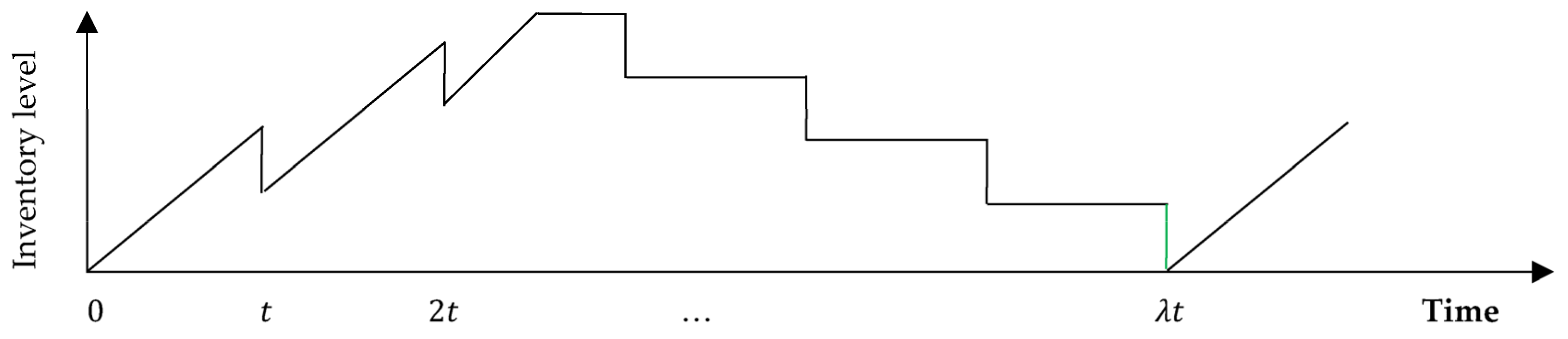
• Any replenishment, $q_1\left(q_s\right)$ ordered at the reorder point, $t_l$ reaches the buyer’s warehouse just prior to the end of that period. However, in the first period of the first cycle, where no items have been manufactured yet, i.e., the buyer’s inventory is zero, the first replenishment, $q_1$ ordered at the beginning of the first period delivers once it has been produced, from which it will arrive to the buyer’s warehouse after a transportation time, $t_{l1}$. In this case, shortages are allowed and fully backordered by time $t_1+t_{l1}$.
• In the first cycle, $p(T_1-t_{l1})\ge 2d{T}_1$, which guarantees that the second lot will reach the buyer’s warehouse no later than time $T_1$.

3.3. The Mathematical Model

Figure 3, Figure 4, Figure 5 and Figure 6 compare this work with the existing literature presented in Figure 1 and Figure 2, Section 1.1. Figure 3 and Figure 4 represent, respectively, the inventory status of the proposed joint model for the vendor and the buyer for the first cycle, whereas Figure 5 and Figure 6 represent, respectively, the inventory status of the proposed joint model for the vendor and the buyer for subsequent cycles. In the proposed joint model, production commences at the beginning of the first cycle at a rate $p$ until time $t_1$, where $q_1$ units have been produced (Figure 3). At this time, i.e., $t_1$, this amount is delivered to the buyer to fully satisfy backordered demand that has been accumulated during production period $t_1$ and transportation period $t_{l1}$, i.e., demand that covers the time $t_1+t_{l1}$ and to satisfy demand until time $T_1$ (Figure 4).

Figure 3. Inventory status of the joint model for the vendor in the first cycle.

Figure 4. Inventory status of the joint model for the buyer in the first cycle $T_{s1}$.

Figure 5. Inventory status of the joint model for the vendor in subsequent cycles.

Figure 6. Inventory status of the joint model for the buyer in subsequent cycles $T_{ss}$.

Note that during the first cycle $T_{s1}$, Figure 3 and Figure 4 indicate that the vendor and the buyer incur a holding cost that applies for $\lambda$ lots, since by time $T_1$, the vendor must then have delivered two lots. That said, the first lot is delivered at time $t_1$, which arrives at the buyer at time $t_1+t_{l1}$, whereas the second lot arrives just before the first lot is consumed, i.e., at time $T_1$. It is worth noting here that such modeling tractability would clear any discrepancy resulting from Figure 1 and Figure 2. More specifically, in Figure 4, the initial inventory level at the beginning of the first cycle is zero, whereas in Figure 6, the inventory level at the beginning of a cycle represents the quantity of the last lot produced in the previous cycle. Similarly, in Figure 3, the vendor delivers the first lot at time $t_1$. In Figure 3 and Figure 5, the last lot produced in the first (subsequent) cycle satisfies the demand for the last period (time $T_1$ ($T_s$) in Figure 4 and Figure 6). However, and for illustrative purposes only, it constitutes the first lot (for time $T_{s-1}$ in Figure 6) in the buyer warehouse in the subsequent cycles, though its associated costs are included in the previous cycle. For holding cost reduction, the re-start-up production time is displaced until time $t_d=T_{s-1}-t_s-t_l$ to allow consuming the last lot that has been replenished to the buyer in the previous cycle. In this case, $t_s=q_s/p$, which satisfies the demand for the buyer during the period $T_s$.

From a mathematical point of view, the last lot produced in the previous cycle constitutes the last lot replenished to the buyer in that same previous cycle. This implies that the costs associated with such a lot should be included in the total cost function of the previous cycle. Moreover, the fact that the inventory fluctuation in the first cycle differs from that in the second cycle would suggest a distinct optimal lot size for the second cycle. From a mathematical and practical point of view, it is often the case that the decision-maker may face a situation that requires input parameters to be adjusted to be compatible with a new policy. Unlike previous works, the lot size produced in a cycle may differ from previous lots. This entails a production policy that generates equal or unequal quantities that are associated with a fixed multiplier for each distinct cycle, and consequently, the production process is dynamic in all cycles, including the first-time interval. As can be seen, Figure 3, Figure 4, Figure 5 and Figure 6 guarantee that the quantity produced for each lot together with its associated multiplier are independent for each cycle, i.e., they are independent from previous cycles. Moreover, Figure 3, Figure 4, Figure 5 and Figure 6 indicate that both the vendor and the buyer incur a holding cost that applies to $\lambda$ lots. Note that in Figure 6, the production, holding, and transportation costs of the first lot (the last lot that has been produced in the previous cycle) are considered for that same previous cycle but have been ignored in cycle $T_{ss}$. Similarly, in Figure 6, the ordering and holding costs of the first lot that has been produced in the previous cycle have been ignored in cycle $T_{ss}$; however, are considered for that same previous cycle. Figure 7 depicts the CO₂ emissions associated with the activities in the vendor and buyer warehouses. The direct emission level related to the buyer occurs due to keeping items in storage, whereas the direct emission level related to the vendor is influenced by producing the required quantity as well as keeping such quantity in storage. The direct emission level related to the vendor also includes the weight of the items delivered to the buyer. The indirect emission level related to the vendor comprises the number of shipments, fuel consumption, the distance between the vendor and the freight, and the distance between the vendor and the buyer.

Figure 7. Classification of CO₂ emissions of the joint model for the vendor and the buyer.

3.3.1. Total Cost Function for the First Cycle under a Centralized Scenario

The inventory level of the first lot depicted in Figure 3 for the vendor is at its maximum, i.e., $q_1$ at time $t_1=q_1/p$, which satisfies demand and shortages.

At time $t_1$, a lot of size $q_1$ units should be replenished to the buyer in a duration of transportation time $t_{l1}$, to satisfy demand and shortages.

This quantity is given by:

$$q_1=d{T}_1,$$

At time $t_1+t_{l1}$, $d(t_1+t_{l1})$ units have been backordered and consequently, the maximum inventory level is $\left(T_1-t_1-t_{l1}\right)d$ units (Figure 4). Therefore, the time required to consume the first lot is given by:

$$\left(T_1-t_1-t_{l1}\right)=\frac{q_1}{d}-\frac{q_1}{p}-t_{l1}$$

(1)

As can be seen, Figure 4 reflects the fact that the buyer’s initial inventory level at the beginning of the first cycle is zero, whereas Figure 3 reflects the fact that the last lot produced in the first cycle constitutes the last lot replenished to the buyer in the first cycle as well. Therefore, we have

$$T_{s1}=\lambda T_1=\frac{\lambda q_1}{d}.$$

(2)

 Remark 1. 

The vendor may use a combination of LTL and TL services to arrange the shipment of the order quantity.

Let $∆=\frac{v_t}{c_t}<v_c$ denotes a quantity for which the cost of transportation by either service is identical and $\delta =\left(\frac{q_1}{v_c}-n\right)$ refers to the proportion of vehicle capacity that needs to be assigned for vehicle $n+1$ if TL service is considered. Therefore, we distinguish two cases:

In case one, the system uses a combination of LTL and TL services to arrange the shipment of the order quantity, i.e., $n$ vehicles of TL service, and transport the rest of the items using LTL service. In this case, $\delta v_c\le ∆⟹v_{t}n+\left(\frac{q_1}{v_c}-n\right)v_c{c}_t$.

In case two, the system uses $n+1$ vehicles of the TL service to arrange the shipment of the order quantity. In this case, $\delta v_c\ge ∆ ⟹v_t\left(n+1\right)$.

Let $\varnothing =1$ denote a pure transportation policy of implementing the TL service, and $\varnothing =0$ refers to a mixed policy for which a combination of LTL and TL services is utilized.

From Figure 3 and Figure 4, and Equations (1) and (2), the holding costs per unit time (see Appendix A) for the buyer and the vendor are, respectively, given by:

$$\frac{h_b{d}^2{t_l}^2}{2\lambda q_1}+\frac{h_b{q}_{1}d}{2\lambda }\left[\frac{d}{p^2}-\frac{2}{p}+\frac{\lambda }{d}\right]+\frac{h_b}{2\lambda }\left[\frac{2d^2{t}_l}{p}-2d{t}_l\right]$$

(3)

$$\frac{h_v{q}_1}{2\lambda }\left[\frac{2d}{p}+{\lambda }^2\left(1-\frac{d}{p}\right)-\lambda \right]-\frac{\left(\lambda -1\right)h_{v}d{t}_l}{\lambda }$$

(4)

 Remark 2. 

In addition to the holding cost, both the buyer and the vendor experience the cost associated with emissions being released while keeping items in storage, which depends on both inventory levels, i.e., Equations (3) and (4) [31,40,56,57].

By Remark 1, the fixed transportation costs per unit time for the vendor is given by:

$$\frac{\varnothing v_t\left(n+1\right)d}{q_1}+\frac{\left(1-\varnothing \right)\left(\left(v_t-v_c{c}_t\right)n+c_t{q}_1\right)d}{q_1}.$$

(5)

The vendor incurs costs associated with emissions from production due to producing $\lambda q_1$ units and delivering this quantity to the buyer. Therefore, the variable transportation and emissions costs per unit of time for the vendor are as follows:

$$\left(v_v+E_{vT}{E}_T\right)d\left(\frac{{T_{f}f}_e}{q_1}+T_v{T}_{w}f\right)+d{E}_v{E}_p{e}^{\frac{{-I}_g}{d}}.$$

(6)

The total amount of emissions generated by the system is given by:

$$\begin{array}{c}{E}_s=\frac{E_e{E}_{wb}{d}^2{t_l}^2}{2\lambda q_1}+\frac{E_e{E}_{wb}{q}_{1}d}{2\lambda }\left[\frac{d}{p^2}-\frac{2}{p}+\frac{\lambda }{d}\right]+\frac{E_e{E}_{wb}}{2\lambda }\left[\frac{2d^2{t}_l}{p}-2d{t}_l\right]+\frac{{E_{e}E}_{wv}{q}_1}{2\lambda }\left[\frac{2d}{p}+{\lambda }^2\left(1-\frac{d}{p}\right)-\lambda \right]-\frac{\left(\lambda -1\right)E_e{E}_{wv}d{t}_l}{\lambda }\hfill \\ +E_{T}d\left(\frac{{T_{f}f}_e}{q_1}+T_v{T}_{w}f\right)+d{E}_p{e}^{\frac{{-I}_g}{d}}.\hfill \end{array}$$

(7)

From which, the cap-and-trade regulations are given by:

$$E_R={E_v(E_s-E_c)}^{-}.$$

(8)

Equation (8) implies that the system earns revenue from selling excess quota if and only if $E_s<E_c$.

Considering the above along with set-up, ordering, and investment cost components, the total cost functions per unit time for the buyer and the vendor are, respectively, given by:

$$W_{s1, b}=\frac{S_{b}d}{q_1}+\frac{(h_b+E_b{E}_e{E}_{wb})d^2{t_l}^2}{2\lambda q_1}+\frac{(h_b+E_b{E}_e{E}_{wb})q_{1}d}{2\lambda }\left[\frac{d}{p^2}-\frac{2}{p}+\frac{\lambda }{d}\right]+\frac{(h_b+E_b{E}_e{E}_{wb})}{2\lambda }\left[\frac{2d^2{t}_l}{p}-2d{t}_l\right].$$

(9)

$$\begin{array}{cc}\hfill W_{s1, v}=& \frac{\left(S_v+I_g\right)d}{\lambda q_1}+\frac{(h_v+E_v{E}_e{E}_{wv})q_1}{2\lambda }\left[\frac{2d}{p}+{\lambda }^2\left(1-\frac{d}{p}\right)-\lambda \right]-\frac{\left(\lambda -1\right)\left(h_v+E_v{E}_e{E}_{wv}\right)d{t}_l}{\lambda }+\frac{\left(1-\varnothing \right)\left(\left(v_t-v_c{c}_t\right)n+c_t{q}_1\right)d}{q_1}+\hfill \\ & \frac{\varnothing v_t\left(n+1\right)d}{q_1}+\left(v_v+E_{vT}{E}_T\right)d\left(\frac{{T_{f}f}_e}{q_1}+T_v{T}_{w}f\right)+d{E}_v{E}_p{e}^{\frac{{-I}_g}{d}}+{E_v(E_s-E_c)}^{-}+c_{v}d.\hfill \end{array}$$

(10)

The term $E_v{E}_p{e}^{\frac{{-I}_g}{d}}$ implies that the higher the investment cost offered by the vendor, the closer the items become greener, and, consequently, the system reaps the benefit of such investment by reducing the cost incurred for emissions generated from production.

Now for simplicity, let $h_b+E_b{E}_e{E}_{wb}=c_1$, $h_v+E_v{E}_e{E}_{wv}=c_2$, and $v_v+E_{vT}{E}_T=c_3$.

Therefore, the total joint cost function per unit time for the buyer and the vendor is given by:

$$\begin{array}{c}{W}_{s1}=W_{s1,b}+W_{s1,v}=\frac{S_{b}d}{q_1}+\frac{\left(S_v+I_g\right)d}{\lambda q_1}+\frac{c_1{d}^2{t_l}^2}{2\lambda q_1}+\frac{c_1{q}_{1}d}{2\lambda }\left[\frac{d}{p^2}-\frac{2}{p}+\frac{\lambda }{d}\right]+\frac{c_1}{2\lambda }\left[\frac{2d^2{t}_l}{p}-2d{t}_l\right]+\frac{c_2{q}_1}{2\lambda }[\frac{2d}{p}+{\lambda }^2\left(1-\frac{d}{p}\right)-\hfill \\ \lambda ]-\frac{c_2\left(\lambda -1\right)d{t}_l}{\lambda }+\frac{\left(1-\varnothing \right)\left(\left(v_t-v_c{c}_t\right)n+c_t{q}_1\right)d}{q_1}+\frac{\varnothing v_t\left(n+1\right)d}{q_1}+c_{3}d\left(\frac{{T_{f}f}_e}{q_1}+T_v{T}_{w}f\right)+d{E}_v{E}_p{e}^{\frac{{-I}_g}{d}}+{E_v(E_s-E_c)}^{-}+c_{v}d\hfill \end{array}$$

(11)

The objective is to find integer values of $\lambda \mathrm{a}\mathrm{n}\mathrm{d} n$ that minimize $W_{s1},$ where $W_{s1}$ is given by Equation (11).

Hence, the objective is to solve the following optimization problem:

$$W_{S1}=\left\{\begin{array}{c}\mathrm{minimize} W_{s1} \mathrm{given} \mathrm{by} \mathrm{Equation} \left(11\right)\\ \mathrm{subject} \mathrm{to} ∆<v_c,\left(\frac{q_1}{v_c}-n\right)\ge 0, n\ge 0, \lambda \ge 1 \\ \varnothing =\left\{\begin{array}{c}1 if \left(\frac{q_1}{v_c}-n\right)v_c\ge ∆ \\ 0 \mathrm{else}\end{array}\right.\\ \\ n \mathrm{and} \lambda \mathrm{intiger} \mathrm{values}\end{array}\right\}$$

(12)

Thus, from Theorem 1 (see Appendix B), a two-step solution approach is provided below:

Step 1:

Find ${\lambda }_{min}\le \lambda \le {\lambda }_{max}$ with an integer value that minimizes either $W_{s1, max}$ or $W_{s1, min}$ given by Equation (A12) or Equation (A13). Alternatively, start with $\lambda =1$ and compute the first three terms of Equation (A12) or Equation (A13) and continue the search by adding 1 each time until Equation (A12) or Equation (A13) attains its minimum.

Step 2:

Using Equation (A11), find $\frac{q_1}{v_c}$, if $\delta v_c\ge ∆$, then set $\varnothing =1$ in Equation (11). Else, i.e., $\delta v_c<∆$, then set $\varnothing =0$ in Equation (11) and compute $E_s$ from Equation (7). Note that $\frac{q_1}{v_c}$ constitutes two numbers, i.e., the integer value of $n$ plus the value of the fraction $\delta$.

In a decentralized, uncoordinated scenario, the buyer orders according to the EOQ formula, and the vendor optimizes the production-inventory policy such that a LFL is replenished for the buyer. In a decentralized, coordinated scenario, the buyer orders according to the EOQ formula, and the vendor in turn must adjust, using $\lambda$, the production-inventory policy, to replenish a multiple of this quantity. In this case, $q_1$ resulted from the EOQ formula of the buyer is used to find $\frac{q_1}{v_c}$, if $\delta v_c\ge ∆$, then set $\varnothing =1$ in Equation (11). Else, i.e., $\delta v_c<∆$, then set $\varnothing =0$ in Equation (11).

3.3.2. Total Cost Function for Subsequent Cycles under a Centralized Scenario

The inventory level of the first lot depicted in Figure 5 for the vendor is at its maximum, i.e., $q_s$ at time $t_s$. Note that the re-start-up production time is displaced until time $t_d$ to allow consuming the last lot that has been replenished to the buyer in the previous cycle. In this case, $t_s=q_s/p$, which satisfies demand for the buyer during the period $T_s$.

At time $t_s$, a lot of size $q_s$ units should be replenished to the buyer to satisfy demand. This quantity is given by:

$$q_s=d{T}_s,$$

where

$$T_{ss}=\lambda T_s=\frac{\lambda q_s}{d}.$$

Considering the above, the total cost functions per unit time (see Appendix A) for the buyer and the vendor are, respectively, given by:

$$W_{ss, b}=\frac{S_{b}d}{q_s}+\frac{c_1{q}_s}{2}=EOQ$$

(13)

$$\begin{array}{c}{W}_{ss, v}=\frac{\left(S_v+I_g\right)d}{\lambda q_s}+\frac{c_2{q}_s}{2}\left[\frac{d}{p}+\left(\lambda -1\right)\left(1-\frac{d}{p}\right)\right]+\frac{\varnothing v_t\left(n+1\right)d}{q_s}+\frac{\left(1-\varnothing \right)\left(\left(v_t-v_c{c}_t\right)n+c_t{q}_s\right)d}{q_s}+c_{3}d\left(\frac{{T_{f}f}_e}{q_s}+T_v{T}_{w}f\right)+\hfill \\ d{E}_v{E}_p{e}^{\frac{{-I}_g}{d}}+{E_v(E_s-E_c)}^{-}+c_{v}d.\hfill \end{array}$$

(14)

Therefore, the total joint cost function per unit time for the buyer and the vendor is given by:

$$\begin{array}{c}{W}_{ss}=\frac{S_{b}d}{q_s}+\frac{\left(S_v+I_g\right)d}{\lambda q_s}+\frac{c_1{q}_s}{2}+\frac{c_2{q}_s}{2}\left[\frac{d}{p}+\left(\lambda -1\right)\left(1-\frac{d}{p}\right)\right]+\frac{\varnothing v_t\left(n+1\right)d}{q_s}+\frac{\left(1-\varnothing \right)\left(\left(v_t-v_c{c}_t\right)n+c_t{q}_s\right)d}{q_s}+\hfill \\ c_{3}d\left(\frac{{T_{f}f}_e}{q_s}+T_v{T}_{w}f\right)+d{E}_v{E}_p{e}^{\frac{{-I}_g}{d}}+{E_v(E_s-E_c)}^{-}+c_{v}d,\hfill \end{array}$$

(15)

where

$$E_s=\frac{E_e{E}_{wb}{q}_s}{2}+\frac{{E_{e}E}_{wv}{q}_s}{2}\left[\frac{d}{p}+\left(\lambda -1\right)\left(1-\frac{d}{p}\right)\right]+E_{T}d\left(\frac{{T_{f}f}_e}{q_s}+T_v{T}_{w}f\right)+d{E}_p{e}^{\frac{{-I}_g}{d}}.$$

(16)

The objective is to find integer values of $\lambda \mathrm{a}\mathrm{n}\mathrm{d} n$ that minimize $W_{ss},$ where $W_{ss}$ is given by Equation (15).

Hence, the objective is to solve the following optimization problem:

$$W_{SS}=\left\{\begin{array}{c}\mathrm{minimise} W_{ss} \mathrm{given} \mathrm{by} \mathrm{Equation} \left(15\right)\\ \mathrm{subject} \mathrm{to} ∆<v_c,\left(\frac{q_s}{v_c}-n\right)\ge 0, n\ge 0, \lambda \ge 1 \\ \varnothing =\left\{\begin{array}{c}1 if \left(\frac{q_s}{v_c}-n\right)v_c\ge ∆ \\ 0 \mathrm{else}\end{array}\right.\\ \\ n \mathrm{and} \lambda \mathrm{intiger} \mathrm{values}\end{array}\right\}$$

(17)

Thus, from Theorem 2 (see Appendix C), a two-step solution approach is provided below:

Step 1:

Find $\lambda \ge 1$ with an integer value that minimizes either $W_{ss, max}$ or $W_{ss, min}$ given by Equation (A19) or Equation (A20). Alternatively, start with $\lambda =1$ and compute the first term of Equation (A19) or Equation (A20) and continue the search by adding 1 each time until Equation (A19) or Equation (A20) attains its minimum.

Step 2:

Using Equation (A17), find $\frac{q_s}{v_c}$, if $\delta v_c\ge ∆$, then set $\varnothing =1$ in Equation (15). Else, i.e., $\delta v_c<∆$, then set $\varnothing =0$ in Equation (15). Note that $\frac{q}{v_c}$ constitutes two numbers, i.e., the integer value of $n$ plus the value of the fraction $\delta$.

4. Numerical Examples

In this section, illustrative examples and special cases that reflect the application of the proposed model are provided.

4.1. Example 1

In this example, we observe the behavior of the system for the set of values listed in Table 3 below.

Table 3. Input parameters for Example 1.

$E_{wb}$	$E_{wv}$	$E_e$	$p$	$E_p$	$v_t$
1.44	1.44	0.0005	8000	1.4	600
kWh/unit/month	kWh/unit/month	ton CO2/kWh	units/month	ton CO2/unit	USD/truck
$v_c$	$c_t$	$T_w$	$T_f$	$T_v$	$v_v$
500	1.5	0.01	80	300	0.75
units/truck	USD/unit	ton/unit	km	km	USD/liter
$f$	$f_e$	$E_T$	$E_c$	$h_v$	$h_b$
0.064	0.32	0.0026	5000	5	3
liters/km/ton	liters/km	ton CO2/liter	tonCO2/month	USD/unit/month	USD/unit/month
$I_g$	$E_b$	$E_v$	$E_{vT}$	$d$	$t_l$
800	2.5	2.5	2.5	3000	0.08
USD/setup	USD/ton CO2	USD/ton CO2	USD/ton CO2	units/month	month
$c_v$	$S_v$	$S_b$
50	1200	400
USD/unit	USD/setup	USD/order

The optimal values of $q_1^{\ast },q_s^{\ast },{\lambda }_1^{\ast },{\lambda }_s^{\ast },n_1^{\ast }, n_s^{\ast },E_{s1}^{\ast },E_{ss}^{\ast },W_{s1}^{\ast }\mathrm{a}\mathrm{n}\mathrm{d} W_{ss}^{\ast }$ are obtained for the first and subsequent cycles and the results are shown in Table 4.

Table 4. Optimal results for the first and subsequent cycles for example 1.

First Cycle	${\mathit{q}}_1^{\mathit{*}}$	${\mathit{\lambda }}_1^{\mathit{*}}$	${\mathit{n}}_1^{\mathit{*}}$	${\mathit{E}}_{\mathit{s}1}^{\mathit{*}}$	${\mathit{W}}_{\mathit{s}1}^{\mathit{*}}$	Mixed Policy	% Saving
With investment	1285	2	2	3219	163,696	$\surd$	2.26%
Without investment	1091	2	2	4202	167,477	$\surd$
Subsequent Cycles	$q_s^{\ast }$	${\lambda }_s^{\ast }$	$n_s^{\ast }$	$E_{ss}^{\ast }$	$W_{ss}^{\ast }$
With investment	1032	2	2	3219	165,910	$\surd$	2.94%
Without investment	1411	1	3	4202	170,927	$\times$

In the first cycle, if the vendor suggests investing in green technology associated with production, then the optimal quantity is $q_1^{\mathrm{*}}=1285 \mathrm{u}\mathrm{n}\mathrm{i}\mathrm{t}\mathrm{s}$ to satisfy both demand and shortages that occurred in the first period, with ${\lambda }_1^{\mathrm{*}}=2$. Note that from Step 2, we have $\frac{q_1^{\mathrm{*}}}{v_c}=\frac{1285}{500}=2.57$, and $∆=\frac{v_t}{c_t}=\frac{600}{1.5}=400 \mathrm{u}\mathrm{n}\mathrm{i}\mathrm{t}\mathrm{s}<v_c=500 \mathrm{u}\mathrm{n}\mathrm{i}\mathrm{t}\mathrm{s}.$ Therefore, $\delta =\left(\frac{q_1^{\mathrm{*}}}{v_c}-n\right)=0.57$, which refers to the proportion of vehicle capacity that needs to be assigned for either policy, i.e., LTL or TL services. Note that $\delta v_c=0.57\times 500=285<∆=400⟹v_{t}n+\left(\frac{q_1^{\mathrm{*}}}{v_c}-n\right)v_c{c}_t$. That is, the vendor should use a combination of LTL and TL services to arrange the shipment of the order quantity. In this case, we set $\mathrm{\varnothing }=0$ and $n=2$ in Equation (11). The monthly cost is $W_{s1}^{\mathrm{*}}=\mathrm{U}\mathrm{S}\mathrm{D} \mathrm{163,696}$, with emissions being generated equals to $E_{s1}^{\mathrm{*}}=3219 \mathrm{t}\mathrm{o}\mathrm{n} {\mathrm{C}\mathrm{O}}_2$. The latter implies that the system earns revenue from the cap-and-trade regulations by selling excess quota, which is given by $E_v\left(E_c-E_s\right)=2.5\left(5000-3219\right)=2.5\left(1781\right)=\mathrm{U}\mathrm{S}\mathrm{D} 4453$. Alternatively, if the vendor suggests not investing in green technology associated with production, then the optimal quantity is $q_1^{\mathrm{*}}=1091 \mathrm{u}\mathrm{n}\mathrm{i}\mathrm{t}\mathrm{s}$ to satisfy both demand and shortages that occurred in the first period, with ${\lambda }_1^{\mathrm{*}}=2$. Therefore, from Step 2, we have $\frac{q_1^{\mathrm{*}}}{v_c}=\frac{1091}{500}=2.182$, and $∆=\frac{v_t}{c_t}=\frac{600}{1.5}=400 \mathrm{u}\mathrm{n}\mathrm{i}\mathrm{t}\mathrm{s}<v_c=500 \mathrm{u}\mathrm{n}\mathrm{i}\mathrm{t}\mathrm{s}.$ Thus, $\delta =\left(\frac{q_1^{\mathrm{*}}}{v_c}-n\right)=0.182⟹\delta v_c=0.182\times 500=91<∆=400⟹v_{t}n+\left(\frac{q_1^{\mathrm{*}}}{v_c}-n\right)v_c{c}_t$. That is, the vendor should use a combination of LTL and TL services to arrange the shipment of the order quantity. In this case, we set $\mathrm{\varnothing }=0$ and $n=2$ in Equation (11). The monthly cost is $W_{s1}^{\mathrm{*}}=\mathrm{U}\mathrm{S}\mathrm{D} \mathrm{167,477}$, with emissions being generated equals to $E_{s1}^{\mathrm{*}}=4202 \mathrm{t}\mathrm{o}\mathrm{n} {\mathrm{C}\mathrm{O}}_2$. In this case, the system earns revenue from the cap-and-trade regulations by selling excess quota, which is given by $E_v\left(E_c-E_s\right)=2.5\left(5000-4202\right)=2.5\left(798\right)=\mathrm{U}\mathrm{S}\mathrm{D} 1995$. Note that this revenue is less than that related to investment. By choosing not to invest, the system also loses the benefit gained by reducing emissions generated from production. This additional revenue is equal to ${\lambda }_1^{\mathrm{*}}{q}_1^{\mathrm{*}}{E}_v\left(E_p-E_p{e}^{\frac{{-I}_g}{d}}\right)=2\times 1285\times 2.5\times 1.4\left(1-e^{\frac{-800}{3000}}\right)=\mathrm{U}\mathrm{S}\mathrm{D} 2106$. Therefore, the total saving achieved due to investment is set equal to $2.26\mathrm{\%}\left(\frac{\mathrm{167,477}-\mathrm{163,696}}{\mathrm{167,477}}\right)\times 100=2.26$. Note that $p\left(T_1-t_{l1}\right)\ge 2d{T}_1$. That is, $p\left(T_1-t_{l1}\right)=8000\times \left(\frac{1285}{3000}-0.08\right)=2786.7>2q_1^{\mathrm{*}}=1285\times 2=2570$ with investment and $p\left(T_1-t_{l1}\right)=8000\times \left(\frac{1091}{3000}-0.08\right)=2269.3>2q_1^{\mathrm{*}}=1091\times 2=2182$ without investment.

In subsequent cycles, if the vendor suggests investing in green technology associated with production, then the optimal quantity is $q_s^{\ast }=1032 \mathrm{u}\mathrm{n}\mathrm{i}\mathrm{t}\mathrm{s}$ to satisfy demand with ${\lambda }_s^{\ast }=2$. Note that from Step 2, we have $\frac{q_s^{\ast }}{v_c}=\frac{1032}{500}=2.064$, and $∆=\frac{v_t}{c_t}=\frac{600}{1.5}=400 \mathrm{u}\mathrm{n}\mathrm{i}\mathrm{t}\mathrm{s}<v_c=500 \mathrm{u}\mathrm{n}\mathrm{i}\mathrm{t}\mathrm{s}.$ Thus, $\delta =\left(\frac{q_s^{\ast }}{v_c}-n\right)=0.064⟹\delta v_c=0.064\times 500=32<∆=400⟹v_{t}n+\left(\frac{q_1^{\ast }}{v_c}-n\right)v_c{c}_t$. That is, the vendor should use a combination of LTL and TL services to arrange the shipment of the order quantity. In this case, we set $\varnothing =0$ and $n=2$ in Equation (15). The monthly cost is $W_{s1}^{\ast }=\mathrm{U}\mathrm{S}\mathrm{D} \mathrm{165,910}$, with emission being generated equals to $E_{s1}^{\ast }=3219 \mathrm{t}\mathrm{o}\mathrm{n} {\mathrm{C}\mathrm{O}}_2$. Note that this amount equals that of the first cycle though the produced quantity is different. The system earns revenue from the cap-and-trade regulations by selling excess quota, which is given by $E_v\left(E_c-E_s\right)=2.5\left(5000-3219\right)=2.5\left(1781\right)=\mathrm{U}\mathrm{S}\mathrm{D} 4453$. If the vendor tends not to invest in green technology associated with production, then the optimal quantity is $q_s^{\ast }=1411 \mathrm{u}\mathrm{n}\mathrm{i}\mathrm{t}\mathrm{s}$ to satisfy demand with ${\lambda }_s^{\ast }=1$. Note that from Step 2, we have $\frac{q_s^{\ast }}{v_c}=\frac{1411}{500}=2.822$, and $∆=\frac{v_t}{c_t}=\frac{600}{1.5}=400 \mathrm{u}\mathrm{n}\mathrm{i}\mathrm{t}\mathrm{s}<v_c=500 \mathrm{u}\mathrm{n}\mathrm{i}\mathrm{t}\mathrm{s}.$ Therefore, $\delta =\left(\frac{q_1^{\ast }}{v_c}-n\right)=0.822$, which refers to the proportion of vehicle capacity that needs to be assigned for either policy, i.e., LTL or TL services. Note that $\delta v_c=0.822\times 500=411>∆=400⟹v_t\left(n+1\right)$. That is, the vendor should use a pure transportation policy of implementing the TL service to arrange the shipment of the order quantity. In this case, we set $\varnothing =1$ and $n=3$ in Equation (15). The monthly cost for no investing is $W_{s1}^{\ast }=\mathrm{U}\mathrm{S}\mathrm{D} \mathrm{170,927}$, with emission being generated equals to $E_{s1}^{\ast }=4202 \mathrm{t}\mathrm{o}\mathrm{n} {\mathrm{C}\mathrm{O}}_2$. Again, the amount of emission is the same as that of the first cycle with a revenue of selling excess quota equals to $\mathrm{U}\mathrm{S}\mathrm{D} 1995$, which is less than that related to the case of investment. As that off the first cycle, choosing not to invest, the system also loses the benefit associated with reducing emission generated from production equals to ${\lambda }_s^{\ast }{q}_s^{\ast }{E}_v\left(E_p-E_p{e}^{\frac{{-I}_g}{d}}\right)=2\times 1302\times 2.5\times 1.4\left(1-e^{\frac{-800}{3000}}\right)=\mathrm{U}\mathrm{S}\mathrm{D} 2133$. Therefore, the total saving achieved due to investment is set equal to $2.94\% \left(\frac{\mathrm{170,927}-\mathrm{165,910}}{\mathrm{170,927}}\right)\times 100=2.94$. Finally, the displaced re-start-up production time is set equal to $t_d=T_{s-1}-t_s-t_l=\frac{1285}{3000}-\frac{1032}{8000}-0.08=0.219 \mathrm{m}\mathrm{o}\mathrm{n}\mathrm{t}\mathrm{h}\approx 7 \mathrm{d}\mathrm{a}\mathrm{y}\mathrm{s}$ when investment is considered. Similarly, $t_d=T_{s-1}-t_s-t_l=\frac{1091}{3000}-\frac{1411}{8000}-0.08=0.107 \mathrm{m}\mathrm{o}\mathrm{n}\mathrm{t}\mathrm{h}\approx 3 \mathrm{d}\mathrm{a}\mathrm{y}\mathrm{s}$ when investment is not considered.

It is clear that $T_{s-1}=T_1\ne T_s$, from which we are sure that the second cycle is independent from the first one. In general, the mathematical formulation guarantees that $T_1 \mathrm{and} T_s$ may or may not be equal. Therefore, the case that $T_{s-1}\ne T_s$ holds for subsequent cycles, which allows the adjustment of the input parameters in any cycle. It is worth noting here that the restriction $p(T_1-t_{l1})\ge 2d{T}_1$ does not apply for subsequent cycles, i.e., it is sufficient to have $p\ge (1+t_l)d$. In this case, the vendor may adjust the production rate, which will not affect the optimal policy because the subsequent cycles are independent of the first cycle and of each other. To see this, suppose that the decision-maker would like to adjust the production rate from 8000 to 4000 to evaluate the consequences of such an adjustment. Table 5 depicts the behavior of the model subject to this adjustment.

Table 5. Optimal results for subsequent cycles for example 1 when $d=4000$ units.

Subsequent Cycles	${\mathit{q}}_{\mathit{s}}^{\mathit{*}}$	${\mathit{\lambda }}_{\mathit{s}}^{\mathit{*}}$	${\mathit{n}}_{\mathit{s}}^{\mathit{*}}$	${\mathit{E}}_{\mathit{s}\mathit{s}}^{\mathit{*}}$	${\mathit{W}}_{\mathit{s}\mathit{s}}^{\mathit{*}}$	Mixed Policy	% Saving
With investment	647	5	1	3219	165,432	$\surd$	0.29%
Without investment	641	4	1	4202	169,473	$\surd$	0.85%

Table 5 reveals that decreasing the production rate from 8000 to 4000 is beneficial since it saves up to $0.29\% \left(\frac{\mathrm{165,910}-\mathrm{165,432}}{\mathrm{165,910}}\right)\times 100=0.29$ with investment and 0.85% without investment when compared with the previous policy. This constitutes evidence that the mathematical formulation generates an optimal solution, that is viable if the values of the input parameters are adjusted for subsequent cycles. Note that the displaced production time is set equal to $t_d=T_{s-1}-t_s-t_l=\frac{1285}{3000}-\frac{647}{4000}-0.08=0.187 \mathrm{m}\mathrm{o}\mathrm{n}\mathrm{t}\mathrm{h}\approx 6 \mathrm{d}\mathrm{a}\mathrm{y}\mathrm{s}$ when investment is considered. Similarly, when investment is not considered, $t_d=T_{s-1}-t_s-t_l=\frac{1091}{3000}-\frac{641}{4000}-0.08=0.123 \mathrm{m}\mathrm{o}\mathrm{n}\mathrm{t}\mathrm{h}\approx 4 \mathrm{d}\mathrm{a}\mathrm{y}\mathrm{s}$.

4.2. Example 2

In this example, we replicate example 1 (the base model) to investigate the sensitivity analysis of the model for the set of parameters listed in Table 3. The most important direct parameters that affect the optimal produced quantity are holding costs, ordering and set-up costs, investment costs, production rates, and demand rates, which are illustrated in Table 6 below.

Table 6. Optimal results for sensitivity analysis for the set of values as listed in Table 3.

Parameter	First Cycle	${\mathit{q}}_1^{\mathit{*}}$	${\mathit{\lambda }}_1^{\mathit{*}}$	${\mathit{n}}_1^{\mathit{*}}$	${\mathit{E}}_{\mathit{s}1}^{\mathit{*}}$	${\mathit{W}}_{\mathit{s}1}^{\mathit{*}}$	Mixed Policy	% Saving
$h_v=h_b=3$	With investment	1473	2	3	3219	164,166	$\surd$	1.63%
	Without investment	2074	1	4	4202	166,890	$\surd$
	Subsequent Cycles	$q_s^{\ast }$	${\lambda }_s^{\ast }$	$n_s^{\ast }$	$E_{ss}^{\ast }$	$W_{ss}^{\ast }$
$h_v=h_b=3$	With investment	1191	2	2	3219	164,921	$\surd$	2.19%
	Without investment	1009	2	2	4202	168,610	$\surd$
	First Cycle	$q_1^{\ast }$	${\lambda }_1^{\ast }$	$n_1^{\ast }$	$E_{s1}^{\ast }$	$W_{s1}^{\ast }$
$S_v=S_b=400$	With investment	1091	2	2	3219	162,561	$\surd$	2.21%
	Without investment	1292	1	2	4202	166,232	$\surd$
	Subsequent Cycles	$q_s^{\ast }$	${\lambda }_s^{\ast }$	$n_s^{\ast }$	$E_{ss}^{\ast }$	$W_{ss}^{\ast }$
$S_v=S_b=400$	With investment	1411	1	3	3219	166,011	$\times$	0.85%
	Without investment	1004	1	2	4202	167,422	$\surd$
	First Cycle	$q_1^{\ast }$	${\lambda }_1^{\ast }$	$n_1^{\ast }$	$E_{s1}^{\ast }$	$W_{s1}^{\ast }$
$d=2000$	With investment	1822	1	3	1878	104,679	$\surd$	4.00%
	Without investment	1493	1	3	2801	109,037	$\times$
	Subsequent Cycles	$q_s^{\ast }$	${\lambda }_s^{\ast }$	$n_s^{\ast }$	$E_{ss}^{\ast }$	$W_{ss}^{\ast }$
$d=2000$	With investment	1508	1	3	1879	105,998	$\surd$	3.25%
	Without investment	1234	1	2	2802	109,557	$\surd$
	First Cycle	$q_1^{\ast }$	${\lambda }_1^{\ast }$	$n_1^{\ast }$	$E_{s1}^{\ast }$	$W_{s1}^{\ast }$
$I_g=1200$	With investment	1371	2	2	2818	162,185	$\surd$	3.12%
	Without investment	1091	2	2	4202	167,477	$\surd$
	Subsequent Cycles	$q_s^{\ast }$	${\lambda }_s^{\ast }$	$n_s^{\ast }$	$E_{ss}^{\ast }$	$W_{ss}^{\ast }$
$I_g=1200$	With investment	1102	2	2	2818	164,520	$\surd$	3.75%
	Without investment	1411	1	3	4202	170,927	$\times$
	First Cycle	$q_1^{\ast }$	${\lambda }_1^{\ast }$	$n_1^{\ast }$	$E_{s1}^{\ast }$	$W_{s1}^{\ast }$
$p=\mathrm{10,000}$	With investment	2223	1	4	3219	163,818	$\surd$	2.27%
	Without investment	1824	1	3	4202	167,617	$\surd$
	Subsequent Cycles	$q_s^{\ast }$	${\lambda }_s^{\ast }$	$n_s^{\ast }$	$E_{ss}^{\ast }$	$W_{ss}^{\ast }$
$p=\mathrm{10,000}$	With investment	1796	1	3	3219	165,859	$\surd$	2.70%
	Without investment	1469	1	3	4202	170,457	$\times$

For equal holding costs, i.e., $h_v=h_b=3$, the optimal produced quantity in the first cycle is higher than that of example 1, though the total minimum cost per unit time is lower because the vendor reduces the holding cost. This also holds for subsequent cycles when the system invests in green production. In the case of no investment, both the optimal produced quantity and the total minimum cost per unit time are lower than those in example 1. We note that the emissions generated are equal in both examples. When $S_v=S_b=400$, both the optimal produced quantity and the total minimum cost per unit time are lower (higher) than those of example 1 in the first cycle (subsequent cycles) for the investment scenario. For the case of no investment, the optimal produced quantity in the first cycle is almost equal to that of example 1, though the total minimum cost per unit time is lower because the vendor reduces the set-up cost. In subsequent cycles, both the optimal produced quantity and the total minimum cost per unit time are lower than those in example 1. We also note that the emissions generated are equal in both examples. When the demand rate decreases from 3000 to 2000, the optimal produced quantity in the first cycle is higher than that of example 1; however, the total minimum cost per unit time and the emissions generated are lower. This also holds in subsequent cycles when the system invests in green production. For the no investment case in subsequent cycles, all optimal values are lower than those of example 1. If the investment cost increases from 800 to 1200, the optimal produced quantity in all cycles is higher than that of example 1 when investment is considered. On the other hand, the total minimum cost per unit time and the emissions generated in all cycles are lower because the vendor increases the investment in green production, where all optimal values in all cycles are identical with those of example 1 when no investment is considered. Finally, if the production rate increases from 8000 to 10,000, the optimal produced quantity and the total minimum cost in the first cycle are higher than those of example 1 when investment is considered. If no investment is considered, the optimal produced quantity is higher than that of example 1; however, the total minimum cost is slightly lower. In subsequent cycles, the optimally produced quantity is higher than that of example 1; however, the total minimum cost is slightly lower.

A comparison between the results obtained in Table 4, Table 5 and Table 6 indicates that the emissions generated by the system are very much related to the demand rate and the investment offered by the vendor. Figure 8, Figure 9 and Figure 10 depict and compare the behavior of the model on the optimal produced quantity, the amount of CO₂ emissions released by the system, and the per-unit-time total cost for the joint system in different settings.

Figure 8. The effect of input parameters on the optimal production quantity for the first and subsequent cycles.

Figure 9. The effect of input parameters on the amount of CO₂ emissions for the first and subsequent cycles.

Figure 10. The effect of input parameters on the total system cost for the first and subsequent cycles.

4.3. Example 3

In this example, a comparison of the proposed model is conducted with the existing literature (e.g., Jaber et al. [9] and Bazan et al. [30]).

For comparison purposes, all additional input parameters that do not affect the optimal quantity and that were not considered by [9,30] have been omitted from the proposed model. Let $S_b=400$, $S_v=1200$, $p=2000$, $d=1000$, $h_v=60$ and $h_b=30$. The cost functions that are compared are, respectively, given by:

$$W_{Es1, max}=W_{Es1, min}=W_{s1}^{\ast }=\frac{\sqrt{2d\left(\lambda S_b+S_v\right)\left(h_b\left[\frac{d^2}{p^2}-\frac{2d}{p}+\lambda \right]+h_v\left[\frac{2d}{p}+{\lambda }^2\left(1-\frac{d}{p}\right)-\lambda \right]\right)}}{\lambda }.$$

(18)

$$W_{ss, max}=W_{ss, min}=W_{ss}^{\ast }=\sqrt{\frac{2d\left(\lambda S_b+S_v\right)\left[h_b+h_v\left[\frac{d}{p}+\left(\lambda -1\right)\left(1-\frac{d}{p}\right)\right]\right]}{\lambda }}.$$

(19)

$$W^{J^{\ast }}=W^{B^{\ast }}=\sqrt{2d\left(\lambda S_b+S_v\right)\left[h_v\left(1-\frac{d}{p}+\frac{1}{\lambda }\right)+\frac{h_b}{\lambda }\right]}.$$

(20)

Equation (18) is a modified version of Equations (A12) and (A13) without emissions and transportation costs, which represents the first cycle of the proposed model. Note that the lead time is ignored, i.e., $t_l=0$ because Jaber et al. [9] and Bazan et al. [30] neglected this lead time. Likewise, Equation (19) is a modified version of Equations (A19) and (A20), which represent the subsequent cycles of the proposed model, where Equation (20) is identical with that of Jaber et al. [9] and Bazan et al. [30].

By substituting the values determined above in Equations (18)–(20) the following results are obtained:

Equation (20) attains its minimum, i.e., $W^{J^{\ast }}=W^{B^{\ast }}=\mathrm{U}\mathrm{S}\mathrm{D} \mathrm{16,970.56}$ with an optimal produced quantity equal to $q_J^{\ast }=$ $q_B^{\ast }=94.28$ when ${\lambda }^{\ast }=3$. Equation (18) attains its minimum, i.e., $W_{s1}^{\ast }=\mathrm{U}\mathrm{S}\mathrm{D} 9874.2$ with an optimal produced quantity equal to $q_1^{\ast }=202.54$ when ${\lambda }_1^{\ast }=2$. Note that $p(T_1-(t_{l1}=0\left)\right)\ge 2d{T}_1⟹p\left(T_1-0\right)=2000\times \left(202.54 /1000\right)=2q_1^{\ast }$. Equation (19) attains its minimum, i.e., $W_{ss}^{\ast }=\mathrm{U}\mathrm{S}\mathrm{D} \mathrm{13,416.41}$ with an optimal produced quantity equal to $q_s^{\ast }=149.07$ when ${\lambda }_s^{\ast }=2$. Therefore, the proposed model produces better results with a dramatic cost reduction. In particular, the cost obtained by Equation (18) is less than that obtained by Equation (20) by $41.82\% \left(\frac{\mathrm{16,970.56}-9874.2}{\mathrm{16,970.56}}\right)\times 100=41.82$. Similarly, the cost obtained by Equation (19) is less than that obtained by Equation (20) by $20.94\% \left(\frac{\mathrm{16,970.56}-\mathrm{13,416.41}}{\mathrm{16,970.56}}\right)\times 100=20.94$. This, indeed, constitutes a key finding for both practitioners and researchers. Moreover, Equation (20) and the other studies in the literature are alike. They implicitly assume that the quantity (e.g., $q_J^{\ast }=$ $q_B^{\ast }=94.28$), which constitutes the initial inventory for the buyer in the first cycle, exists even though the vendor has not yet commenced production. This can be attributed to the fact that the mathematical modeling has been formulated based on a finite planning horizon. However, the fact remains that the initial inventory at the buyer’s site is zero. Another issue associated with such mathematical modeling is that the values of the input parameters remain static indefinitely. This implies a production policy that generates an equal quantity that is associated with a fixed multiplier in all cycles, and consequently, the production process is static in all cycles, including the first-time interval (e.g., $q_J^{\ast }=$ $q_B^{\ast }=94.28$) remains static indefinitely. On the other hand, it is often the case that the input parameters are subject to adjustment due to a plethora of endogenous and/or exogenous factors that may force the system to adjust the input parameters. Therefore, the proposed model not only considers the abovementioned issues but also generates better results with a dramatic cost reduction (see also Example 1). Further, the re-start-up production time is displaced for more holding cost reduction.

It is worth noting here that Equation (20) could produce lower cost if for example $p$ is set equal to $p=1100\ge d=1000$. In this case, Equation (20) attains its minimum, i.e., $W^{J^{\ast }}=W^{B^{\ast }}=\mathrm{U}\mathrm{S}\mathrm{D} \mathrm{12,103.45}$ with an optimal produced quantity equals to $q_J^{\ast }=$ $q_B^{\ast }=94.42$ when ${\lambda }^{\ast }=7$. Equation (18) attains its previous minimum cost, i.e., $W_{s1}^{\ast }=\mathrm{U}\mathrm{S}\mathrm{D} 9874.2$ with an optimal produced quantity equals to $q_1^{\ast }=202.54$ when ${\lambda }_1^{\ast }=2$ and $p=2000$. This is so, to ensure shortages do not occur for period 2 where $p(T_1-(t_{l1}=0\left)\right)\ge 2d{T}_1⟹p\left(T_1-0\right)=2000\times \left(202.54 /1000\right)=2d{T}_1=2q_1^{\ast }$. However, this does not apply for subsequent cycles. Therefore, Equation (19) attains its minimum, i.e., $W_{ss}^{\ast }=\mathrm{U}\mathrm{S}\mathrm{D} \mathrm{11,576.96}$ with an optimal produced quantity equals to $q_s^{\ast }=98.71$ when ${\lambda }_s^{\ast }=7$ and $p=1100$. In this case, the cost obtained by Equation (18) is less than that of Equation (20) by $18.42\% \left(\frac{\mathrm{12,103.45}-9874.2}{\mathrm{12,103.45}}\right)\times 100=18.42$. Similarly, the cost obtained by Equation (19) is less than that of Equation (20) by $4.35\% \left(\frac{\mathrm{12,103.45}-\mathrm{11,576.96}}{\mathrm{12,103.45}}\right)\times 100=4.35$.

5. Model Overview and Managerial Insights

Unlike the classical formulation of the joint vendor-buyer model, which assumes a finite planning horizon and ignores the impact of the first cycle, the proposed model considers the first-time interval in the mathematical formulation. Moreover, the proposed model guarantees that the optimal produced quantity together with its associated multiplier are independent for each cycle, i.e., each cycle is independent from the previous one. The re-start-up production time for subsequent cycles commences only at the time required to produce and replenish the first lot, which implies further cost reduction. That is, it prevents keeping inventory related to the vendor for the unnecessary time associated with the time elapsing for the consumption of the last lot that has been shipped to the buyer. A rigorous heuristic method is utilized to reduce the computational effort dramatically. This method is cobbled together with a mixed transportation policy of LT and LTL services, where a solution technique for a MINLP problem is proposed to obtain a global optimal solution for the joint model. Accordingly, the condition that renders the cost of transportation by either service identical is derived to establish the relation of the mixed strategy required to be implemented in the mathematical formulation. This paper showed and proved that ignorance of the physical transportation cost does not affect the optimal quantity produced. The (term of the proposed model that has been addressed for compassion purposes (Example 3)), represents the base model, which rectifies the base model adopted by the existing literature. Therefore, it can be further adopted to rectify several existing models disseminated from the rectified model, which may interest researchers. This can be justified by the fact that the base proposed model generates an optimal quantity with a considerable total cost reduction when compared with the best scenario in favor of the existing literature.

The results indicate that the first cycle significantly impacts the optimal production policy. The proposed model generates an optimal produced quantity for the first cycle (subsequent cycles), with more than $18.42\%$ (4.35%) less total system cost when compared with the pest scenario in favor of the existing literature, i.e., at a production rate slightly greater than the demand rate. Moreover, such a percentage of total system cost reduction increases as the production rate increases. The proposed model not only produces better results but also offers the opportunity to adjust the input parameters for subsequent cycles. The viability and validity of the model are ascertained, and consequently, it generates optimal results, whether the input parameters change their values for each cycle or remain static. The results obtained indicate that the emissions generated by the system are very much related to the demand rate and the amount of investment in green production. The total savings that can be achieved through investment is beneficial for the system. That is, the higher the investment in green production, the higher the revenue gained by reducing emission costs as well as earning further revenue from the cap-and-trade regulations by selling excess quota. The proposed model enables the system to reflect economic, social, and environmental interests, and consequently, the system emphasizes sustainability. The higher the investment cost offered by the system, the closer the items become greener and, consequently, the system becomes more sustainable. The results indicate that the increase in the production rate increases the optimal produced quantity with a slight increase in the total system cost per unit time and subsequently impacts economic opportunities with no influence on the amount of emissions released into the environment. The proposed model combines LTL and TL transportation strategies in the mathematical formulation for further cost reduction.

6. Discussion

Sustainable supply chain management is challenging in terms of addressing economic, social, and environmental interests. Although the concept of the VMI model for a JELS policy is not new, the mathematical modeling of such a policy may still have a space for further contributions. For instance, the classical formulation of the joint VMI model assumes a production policy that generates an equal quantity that is associated with a fixed multiplier in all cycles, and consequently, the production process is static in all cycles. This can be justified by the fact that the mathematical formulation is based on an infinite planning horizon and ignores the impact of the first cycle. The classical formulation of the joint vendor-buyer inventory model is associated with another implicit assumption: that input parameters remain static indefinitely. In practice, however, there exist a plethora of factors that may force the decision-maker to adjust input parameters. For example, adaptation of a new policy due to acquired new knowledge, price fluctuations, the dynamic nature of demand and production rates, machine maintenance scheduling activities, or periodic review applications may raise such an adjustment. Therefore, if the decision-maker would like to deviate from the current policy, then the suggested solution obtained by the classical approach cannot be used as the right policy for subsequent cycles.

This paper is concerned with the mathematical formulation of a vendor-buyer inventory model for a JELS policy, considering the abovementioned issues. Accordingly, two mathematical models are developed for a VMI. The first model underlies the first cycle, while the second underlies subsequent cycles. Each model considers investment in green production, energy used for keeping items in storage, and carbon emissions from production, storage, and transportation activities under the carbon cap-and-trade policy. LTL and TL are two common cost structures for freight, and consequently, the proposed model combines these two transportation strategies in the mathematical formulation. To reduce the per-unit-time total cost function, the re-start-up production time for subsequent cycles is displaced up to the time required to produce and deliver the first lot. Moreover, this paper developed a rigorous heuristic method to dramatically reduce the computational effort by obtaining a global optimal solution for a joint supply chain and inventory management model for a given product.

Illustrative examples indicate that the first cycle significantly impacts the optimal production policy. The proposed model generates distinct optimal results associated with the first and subsequent cycles. The viability and validity of the model have been emphasized where the model generates optimal results, whether the input parameters change their values for each cycle or remain static. The impact of adjusting the input parameters for sensitivity analysis purposes and some important opportunities for decision-makers are evaluated. For example, the results obtained indicate that the emissions generated by the system are very much related to the demand rate and the amount of investment in green production. The results also indicate that the higher the investment in green production, the higher the revenue gained by reducing emission costs as well as earning further revenue from the cap-and-trade regulations by selling excess quota. Therefore, the proposed model enables the system to reflect economic, social, and environmental interests, and consequently, the system emphasizes sustainability. The system reaps the benefit of investing in green production, i.e., the higher the investment cost offered by the system, the closer the items become greener and, consequently, the system becomes more sustainable. One of the main findings is that the increase in the production rate increases the optimal produced quantity with a slight increase in the total system cost per unit time. Therefore, it impacts economic opportunities without having any influence on the amount of emissions released into the environment.

A comparison with the best scenario in favor of the existing literature showed that the proposed model generates an optimal produced quantity with $18.42\%$ (4.35%) less total system cost for the first cycle (subsequent cycles). Moreover, such a percentage increases as the production rate increases. Further, the proposed model not only produces better results but also offers the opportunity to adjust the input parameters for subsequent cycles. This, indeed, will be perceived as an important finding for both academics and practitioners.

7. Conclusions and Further Research

In this paper, a vendor-buyer inventory model for a JELS policy is presented. The proposed model considers the mathematical issues associated with the classical formulation of the joint vendor-buyer model. Moreover, it is a viable solution and considers the dynamic nature of demand and production rates or price fluctuations, which is often the case in real-life settings. That is, if the decision-maker would like to deviate from the current policy, then the proposed model guarantees that the optimal produced quantity together with its associated multiplier are independent for each cycle, i.e., it generates distinct optimal results for subsequent cycles. The re-start-up production time for subsequent cycles implies further cost reduction by not keeping inventory related to the vendor for unnecessary time associated with the consumption time of the last lot that has been shipped to the buyer. A mixed transportation policy of LT and LTL services is considered in the mathematical formulation, where a solution technique for a MINLP problem is proposed to obtain a global optimal solution for the joint model. In particular, the model offers the condition that the cost of transportation by either service is identical, from which the relation of the mixed strategy is derived. This paper showed and proved that ignorance of the physical transportation cost does not affect the optimal quantity produced. The (term of the proposed model that has been addressed for compassion purposes (Example 3)), represents the base model, which rectifies the base model adopted by the existing literature. Therefore, it can be further adopted to rectify several existing models that account for extensions based on the rectified model and that may interest researchers. This can be justified by the fact that the base proposed model generates an optimal quantity with a considerable total cost reduction when compared with the best scenario in favor of the existing literature. Further, the proposed model not only produces better results but also offers the opportunity to adjust the input parameters for subsequent cycles, where each cycle is independent from the previous one.

Based on the findings of this paper, it seems plausible to extend the model for a hybrid production system that combines both green and regular production activities. In addition, the formulation of an imperfect production facility where defective items are subject to reworking is also possible. An interesting line of further research may include the formulation of a reverse logistics inventory system considering manufacturing, remanufacturing, and transportation, along with GHG emissions. The incorporation of learning and forgetting curves into the production rate is another interesting line of inquiry. Another research option is the formulation of a general inventory model, considering demand, production, and deterioration rates as general functions of time. Further, extending the model while accounting for different penalties for exceeding emissions limits is also possible. Finally, the proposed idea of considering the first-time interval in the mathematical formulation can be further extended to be implemented in several interesting further inquiries related to JELS inventory mathematical modeling.

References

- Alamri, A.A. A Sustainable Closed-Loop Supply Chains Inventory Model Considering Optimal Number of Remanufacturing Times. Sustainability 2023, 15, 9517. [Google Scholar] [CrossRef]
- Alamri, A.A. Exploring the Effect of the First Cycle on the Economic Production Quantity Repair and Waste Disposal Model. Appl. Math. Model. 2021, 89, 519–540. [Google Scholar] [CrossRef]
- Benjaafar, S.; Li, Y.; Daskin, M. Carbon Footprint and the Management of Supply Chains: Insights from Simple Models. IEEE Trans. Autom. Sci. Eng. 2012, 10, 99–116. [Google Scholar] [CrossRef]
- Wang, X.J.; Choi, S.H. Impacts of Carbon Emission Reduction Mechanisms on Uncertain Make-To-Order Manufacturing. Int. J. Prod. Res. 2016, 54, 3311–3328. [Google Scholar] [CrossRef]
- EPA. Carbon Pollution from Transportation. U.S. Environmental Protection Agency. 2022. Available online: https://www.epa.gov/transportation-air-pollution-and-climate-change/carbon-pollution-transportation#transportation (accessed on 17 July 2023).
- Jaber, M.Y.; Zolfaghari, S. Quantitative Models for Centralised Supply Chain Coordination. In Supply Chains: Theory and Applications; InTech Open: Rijeka, Croatia, 2008; pp. 307–338. [Google Scholar]
- Glock, C.H. The Joint Economic Lot Size Problem: A Review. Int. J. Prod. Econ. 2012, 135, 671–686. [Google Scholar] [CrossRef]
- Rekik, Y.; Syntetos, A.; Jemai, Z. An E-Retailing Supply Chain Subject to Inventory Inaccuracies. Int. J. Prod. Econ. 2015, 167, 139–155. [Google Scholar] [CrossRef]
- Jaber, M.Y.; Glock, C.H.; El Saadany, A.M.A. Supply Chain Coordination with Emissions Reduction Incentives. Int. J. Prod. Res. 2013, 51, 69–82. [Google Scholar] [CrossRef]
- Lippman, S.A. Economic Order Quantities and Multiple Set-up Costs. Manag. Sci. 1971, 18, 39–47. [Google Scholar] [CrossRef]
- Konur, D. Carbon Constrained Integrated Inventory Control and Truckload Transportation with Heterogeneous Freight Trucks. Int. J. Prod. Econ. 2014, 153, 268–279. [Google Scholar] [CrossRef]
- Venkatachalam, S.; Narayanan, A. Efficient Formulation and Heuristics for Multi-Item Single Source Ordering Problem with Transportation Cost. Int. J. Prod. Res. 2016, 54, 4087–4103. [Google Scholar] [CrossRef]
- Damert, M.; Feng, Y.; Zhu, Q.; Baumgartner, R.J. Motivating Low-Carbon Initiatives among Suppliers: The Role of Risk and Opportunity Perception. Resour. Conserv. Recycl. 2018, 136, 276–286. [Google Scholar] [CrossRef]
- Das, C.; Jharkharia, S. Low Carbon Supply Chain: A State-of-the-Art Literature Review. J. Manuf. Technol. Manag. 2018, 29, 398–428. [Google Scholar] [CrossRef]
- Banerjee, A. A Joint Economic-lot-size Model for Purchaser and Vendor. Decis. Sci. 1986, 17, 292–311. [Google Scholar] [CrossRef]
- Dong, Y.; Xu, K. A Supply Chain Model of Vendor Managed Inventory. Transp. Res. E Logist. Transp. Rev. 2002, 38, 75–95. [Google Scholar] [CrossRef]
- Devy, N.L.; Ai, T.J.; Astanti, R.D. A Joint Replenishment Inventory Model with Lost Sales. IOP Conf. Ser. Mater. Sci. Eng. 2018, 337, 12018. [Google Scholar] [CrossRef]
- Utama, D.M.; Santoso, I.; Hendrawan, Y.; Dania, W.A.P. Integrated Procurement-Production Inventory Model in Supply Chain: A Systematic Review. Oper. Res. Perspect. 2022, 9, 100221. [Google Scholar] [CrossRef]
- Nugroho, A.; Wee, H.M. Supply Chain Coordination under Vendor Managed Inventory System Considering Carbon Emission for Imperfect Quality Deteriorating Items. In Proceedings of the 9th International Conference on Operations and Supply Chain Management, Ho Chi Minh City, Vietnam, 15 December 2019; pp. 15–18. [Google Scholar]
- Bai, Q.; Jin, M.; Xu, X. Effects of Carbon Emission Reduction on Supply Chain Coordination with Vendor-Managed Deteriorating Product Inventory. Int. J. Prod. Econ. 2019, 208, 83–99. [Google Scholar] [CrossRef]
- Goyal, S.K. An Integrated Inventory Model for a Single Supplier-Single Customer Problem. Int. J. Prod. Res. 1977, 15, 107–111. [Google Scholar] [CrossRef]
- Goyal, S.K. “A Joint Economic-lot-size Model for Purchaser and Vendor”: A Comment. Decis. Sci. 1988, 19, 236–241. [Google Scholar] [CrossRef]
- Gunasekaran, A.; Irani, Z.; Papadopoulos, T. Modelling and Analysis of Sustainable Operations Management: Certain Investigations for Research and Applications. J. Oper. Res. Soc. 2014, 65, 806–823. [Google Scholar] [CrossRef]
- Taleizadeh, A.A.; Soleymanfar, V.R.; Govindan, K. Sustainable Economic Production Quantity Models for Inventory Systems with Shortage. J. Clean. Prod. 2018, 174, 1011–1020. [Google Scholar] [CrossRef]
- Montabon, F.; Pagell, M.; Wu, Z. Making Sustainability Sustainable. J. Supply Chain. Manag. 2016, 52, 11–27. [Google Scholar] [CrossRef]
- Wahab, M.I.M.; Mamun, S.M.H.; Ongkunaruk, P. EOQ Models for a Coordinated Two-Level International Supply Chain Considering Imperfect Items and Environmental Impact. Int. J. Prod. Econ. 2011, 134, 151–158. [Google Scholar] [CrossRef]
- Hua, G.; Cheng, T.C.E.; Wang, S. Managing Carbon Footprints in Inventory Management. Int. J. Prod. Econ. 2011, 132, 178–185. [Google Scholar] [CrossRef]
- Wangsa, I. Greenhouse Gas Penalty and Incentive Policies for a Joint Economic Lot Size Model with Industrial and Transport Emissions. Int. J. Ind. Eng. Comput. 2017, 8, 453–480. [Google Scholar]
- Gautam, P.; Kishore, A.; Khanna, A.; Jaggi, C.K. Strategic Defect Management for a Sustainable Green Supply Chain. J. Clean. Prod. 2019, 233, 226–241. [Google Scholar] [CrossRef]
- Bazan, E.; Jaber, M.Y.; Zanoni, S. Supply Chain Models with Greenhouse Gases Emissions, Energy Usage and Different Coordination Decisions. Appl. Math. Model. 2015, 39, 5131–5151. [Google Scholar] [CrossRef]
- Halat, K.; Hafezalkotob, A. Modeling Carbon Regulation Policies in Inventory Decisions of a Multi-Stage Green Supply Chain: A Game Theory Approach. Comput. Ind. Eng. 2019, 128, 807–830. [Google Scholar] [CrossRef]
- Ghosh, A.; Jha, J.K.; Sarmah, S.P. Optimal Lot-Sizing under Strict Carbon Cap Policy Considering Stochastic Demand. Appl. Math. Model. 2017, 44, 688–704. [Google Scholar] [CrossRef]
- Hariga, M.; As’ad, R.; Shamayleh, A. Integrated Economic and Environmental Models for a Multi Stage Cold Supply Chain under Carbon Tax Regulation. J. Clean. Prod. 2017, 166, 1357–1371. [Google Scholar] [CrossRef]
- Ganesh Kumar, M.; Uthayakumar, R. Modelling on Vendor-Managed Inventory Policies with Equal and Unequal Shipments under GHG Emission-Trading Scheme. Int. J. Prod. Res. 2019, 57, 3362–3381. [Google Scholar] [CrossRef]
- Chen, X.; Benjaafar, S.; Elomri, A. The Carbon-Constrained EOQ. Oper. Res. Lett. 2013, 41, 172–179. [Google Scholar] [CrossRef]
- Saga, R.S.; Jauhari, W.A.; Laksono, P.W.; Dwicahyani, A.R. Investigating Carbon Emissions in a Production-Inventory Model under Imperfect Production, Inspection Errors and Service-Level Constraint. Int. J. Logist. Syst. Manag. 2019, 34, 29–55. [Google Scholar] [CrossRef]
- Zanoni, S.; Mazzoldi, L.; Jaber, M.Y. Vendor-Managed Inventory with Consignment Stock Agreement for Single Vendor–Single Buyer under the Emission-Trading Scheme. Int. J. Prod. Res. 2014, 52, 20–31. [Google Scholar] [CrossRef]
- Huang, Y.-S.; Fang, C.-C.; Lin, Y.-A. Inventory Management in Supply Chains with Consideration of Logistics, Green Investment and Different Carbon Emissions Policies. Comput. Ind. Eng. 2020, 139, 106207. [Google Scholar] [CrossRef]
- Malik, A.I.; Kim, B.S. A Constrained Production System Involving Production Flexibility and Carbon Emissions. Mathematics 2020, 8, 275. [Google Scholar] [CrossRef]
- Astanti, R.D.; Daryanto, Y.; Dewa, P.K. Low-Carbon Supply Chain Model under a Vendor-Managed Inventory Partnership and Carbon Cap-and-Trade Policy. J. Open Innov. Technol. Mark. Complex. 2022, 8, 30. [Google Scholar] [CrossRef]
- Turken, N.; Geda, A.; Takasi, V.D.G. The Impact of Co-Location in Emissions Regulation Clusters on Traditional and Vendor Managed Supply Chain Inventory Decisions. Ann. Oper. Res. 2021, 1–50. [Google Scholar] [CrossRef]
- Sarkar, B.; Saren, S. Product Inspection Policy for an Imperfect Production System with Inspection Errors and Warranty Cost. Eur. J. Oper. Res. 2016, 248, 263–271. [Google Scholar] [CrossRef]
- Rad, M.A.; Khoshalhan, F.; Glock, C.H. Optimal Production and Distribution Policies for a Two-Stage Supply Chain with Imperfect Items and Price-and Advertisement-Sensitive Demand: A Note. Appl. Math. Model. 2018, 57, 625–632. [Google Scholar] [CrossRef]
- Kim, M.-S.; Kim, J.-S.; Sarkar, B.; Sarkar, M.; Iqbal, M.W. An Improved Way to Calculate Imperfect Items during Long-Run Production in an Integrated Inventory Model with Backorders. J. Manuf. Syst. 2018, 47, 153–167. [Google Scholar] [CrossRef]
- De Giovanni, P.; Karray, S.; Martín-Herrán, G. Vendor Management Inventory with Consignment Contracts and the Benefits of Cooperative Advertising. Eur. J. Oper. Res. 2019, 272, 465–480. [Google Scholar] [CrossRef]
- Phan, D.A.; Vo, T.L.H.; Lai, A.N.; Nguyen, T.L.A. Coordinating Contracts for VMI Systems under Manufacturer-CSR and Retailer-Marketing Efforts. Int. J. Prod. Econ. 2019, 211, 98–118. [Google Scholar] [CrossRef]
- Ben-Daya, M.; As’ad, R.; Nabi, K.A. A Single-Vendor Multi-Buyer Production Remanufacturing Inventory System under a Centralized Consignment Arrangement. Comput. Ind. Eng. 2019, 135, 10–27. [Google Scholar] [CrossRef]
- Tarhini, H.; Karam, M.; Jaber, M.Y. An Integrated Single-Vendor Multi-Buyer Production Inventory Model with Transshipments between Buyers. Int. J. Prod. Econ. 2020, 225, 107568. [Google Scholar] [CrossRef]
- Dey, O.; Giri, B.C. A New Approach to Deal with Learning in Inspection in an Integrated Vendor-Buyer Model with Imperfect Production Process. Comput. Ind. Eng. 2019, 131, 515–523. [Google Scholar] [CrossRef]
- Giri, B.C.; Chakraborty, A.; Maiti, T. Consignment Stock Policy with Unequal Shipments and Process Unreliability for a Two-Level Supply Chain. Int. J. Prod. Res. 2017, 55, 2489–2505. [Google Scholar] [CrossRef]
- Jauhari, W.A.; Sofiana, A.; Kurdhi, N.A.; Laksono, P.W. An Integrated Inventory Model for Supplier-Manufacturer-Retailer System with Imperfect Quality and Inspection Errors. Int. J. Logist. Syst. Manag. 2016, 24, 383–407. [Google Scholar]
- Khan, M.; Hussain, M.; Cárdenas-Barrón, L.E. Learning and Screening Errors in an EPQ Inventory Model for Supply Chains with Stochastic Lead Time Demands. Int. J. Prod. Res. 2017, 55, 4816–4832. [Google Scholar] [CrossRef]
- Pal, S.; Mahapatra, G.S. A Manufacturing-Oriented Supply Chain Model for Imperfect Quality with Inspection Errors, Stochastic Demand under Rework and Shortages. Comput. Ind. Eng. 2017, 106, 299–314. [Google Scholar] [CrossRef]
- Tiwari, S.; Kazemi, N.; Modak, N.M.; Cárdenas-Barrón, L.E.; Sarkar, S. The Effect of Human Errors on an Integrated Stochastic Supply Chain Model with Setup Cost Reduction and Backorder Price Discount. Int. J. Prod. Econ. 2020, 226, 107643. [Google Scholar] [CrossRef]
- Jaggi, C.K.; Tiwari, S.; Shafi, A.A. Effect of Deterioration on Two-Warehouse Inventory Model with Imperfect Quality. Comput. Ind. Eng. 2015, 88, 378–385. [Google Scholar] [CrossRef]
- Bouchery, Y.; Ghaffari, A.; Jemai, Z.; Tan, T. Impact of Coordination on Costs and Carbon Emissions for a Two-Echelon Serial Economic Order Quantity Problem. Eur. J. Oper. Res. 2017, 260, 520–533. [Google Scholar] [CrossRef]
- Kazemi, N.; Abdul-Rashid, S.H.; Ghazilla, R.A.R.; Shekarian, E.; Zanoni, S. Economic Order Quantity Models for Items with Imperfect Quality and Emission Considerations. Int. J. Syst. Sci. Oper. Logist. 2018, 5, 99–115. [Google Scholar] [CrossRef]
Disclaimer/Publisher’s Note: The statements, opinions and data contained in all publications are solely those of the individual author(s) and contributor(s) and not of MDPI and/or the editor(s). MDPI and/or the editor(s) disclaim responsibility for any injury to people or property resulting from any ideas, methods, instructions or products referred to in the content. |
© 2023 by the author. Licensee MDPI, Basel, Switzerland. This article is an open access article distributed under the terms and conditions of the Creative Commons Attribution (CC BY) license (https://creativecommons.org/licenses/by/4.0/).