Article

Impact of Second-Tier Container Port Facilities on Drayage Operation

1
Operations Research, United Postal Service, Timonium MD 21093, USA
2
Department of Civil and Environmental Engineering, University of South Carolina, Columbia, SC 29208, USA
3
The Tioga Group, Inc., Moraga, CA 94556, USA
*
Author to whom correspondence should be addressed.
Logistics 2022, 6(4), 68; https://doi.org/10.3390/logistics6040068
Submission received: 23 August 2022 / Revised: 14 September 2022 / Accepted: 19 September 2022 / Published: 27 September 2022
(This article belongs to the Special Issue Optimization and Management in Maritime Transportation)

Abstract

:
Background: An increasing number of container and chassis staging, “dray-off”, drop yard, and depot facilities are being established outside of North American marine container terminals. The increased use of these “second-tier” facilities implies that there must be some capacity, delivery time, service, or reliability benefit that offset the additional cost and complexity. Methods: This paper builds on the previously developed integrated drayage scheduling model to determine the impact of second-tier port facilities on drayage operation. It modifies the previously developed model by incorporating the following features: (1) trucks do not have to wait at customers’ locations during the import unloading and export loading operations; (2) drayage operations can include a drop yard (i.e., second-tier facility) for picking up or/and dropping off loaded containers outside the marine container terminal; and (3) a customer is allowed to request any of the following jobs: pick up an empty container, pick up a loaded container, drop off an empty container, and drop off a loaded container. Results: The results indicated that by moving the location of import pickup and export delivery from inside the marine container terminal to a location outside the terminal, the efficiency of drayage operation could increase. Additionally, when import pickup and export delivery take place inside the marine container terminal, the most efficient location for the chassis yard and empty container depot is inside the terminal. However, when the location of import pickup and/or export delivery are outside the terminal, the most efficient location for the chassis yard and empty container depot is also outside the terminal. Conclusions: The modeling results suggest that in addition to adding reserved capacity for marine terminals or as buffers to reconcile the preferred delivery times of importers, the second-tier facilities could also yield operational savings. However, the potential drayage efficiencies depend heavily on shorter queuing and turn time at these less-complex facilities compared to marine container terminals. Lastly, the modeling results suggest that the observed evolution of North American marine container terminals from self-contained entities into multi-tier systems is likely to continue to add additional capacities to accommodate container trade growth. This finding has important implications for regions and communities concerned over the impact of growing container ports.

1. Introduction

There is an observable trend in the North American container port industry toward the establishment of auxiliary or satellite facilities to store, stage, or transfer loaded containers, empty containers, and bare container chassis outside port container terminals [1]. For example, the STOR (Short Term Overflow Resource) yard was open for business at the Port of Long Beach (PoLB) in December 2020. The intent of STOR as the PoLB Executive Director noted [1] is that “It frees up space at the marine terminals and allows our industry partners to prioritize the movement of their containers in and out of the port so customers can get their products where they need to go when they need to move them.” On the surface, these “second-tier” facilities would appear to duplicate the functions of the marine container terminals themselves, and to add steps to the import or export handling process. This trend may seem counter-intuitive in an industry obsessed with efficiency. The increased use of second-tier facilities implies that there must be some capacity, delivery time, service, or reliability benefit that offset the additional cost and complexity. To date, no study has analyzed the impact of second-tier facilities and provided guidance to port authorities and terminal operators on how best to incorporate second-tier facilities into their marine container ports. This paper seeks to contribute to this understanding and to develop a mathematical program to assist with the analysis.
The drayage scheduling problem is a variation of the pickup-and-delivery problem (PDP) in which vehicle capacity equals one, since it involves picking up a container from one place and delivering it to another. Several studies have formulated the drayage problem as a PDP. These studies include the work of Wang and Regan [2], Ileri et al. [3], Imai et al. [4], Caris and Janssen [5], and Nossack and Pesch [6]. Since drayage operation involves the movement of the tractor, loaded container, empty container, and chassis, some studies have focused on developing drayage scheduling models that consider the movement of loaded and empty containers jointly. These studies include the work of Zhang et al. [7,8,9], Braekers et al. [10,11], and Shiri and Huynh [12]. In recent years, a number of studies have addressed the drayage problem considering different container size. These studies include the work of Vidović et al. [13,14], Popović et al. [15], Zhang et al. [16], and Funke and Kopfer [17]. Drayage studies that considered time-window constraints at marine container terminals (via a truck appointment system) include the work by Namboothiri and Erera [18], and Shiri and Huynh [19]. Cheung and Hange [20], Cheung et al. [21] and Shiri et al. [22] have addressed the dynamic or stochastic version of the drayage problem. A few studies have considered the collaboration between drayage companies. These studies include the work of Sterzik et al. [23] and Wang and Kopfer [24]. A complete review of drayage studies can be found in the works of Shiri and Huynh [12,19], Wang and Kopfer [24], and Braekers et al. [10]. To date, no study has examined the impact of drop yards and other second-tier facilities as a whole on drayage operation, with the exception of the work by Lei and Church [25] who analyzed the option of establishing empty storage yards away from the port. To our knowledge, this study is the first to examine the effect of having the second-tier facilities (import pickup, export delivery, chassis yard, and empty container depot) on or off the marine container terminal.
To determine the impact of second-tier facilities on drayage operation this study builds on a previously developed drayage scheduling model by Shiri and Huynh [12]. This model is a mixed-integer quadratic programming model that solves the scheduling of tractor, loaded container, empty container, and chassis in an integrated manner. For this study, the following modifications are made to the model: (1) trucks do not have to wait at customers’ locations during the import unloading and export loading operations; (2) drayage operations can include a drop yard (i.e., second-tier facility) for picking up or/and dropping off loaded containers outside the marine container terminal; and (3) the job requests by customers are extended to include empty container pickup, loaded container pickup, empty container delivery, and loaded container delivery. To solve this model, a reactive tabu search algorithm (RTS) combined with an insertion heuristic developed by the authors is used. The impact of second-tier facilities on drayage operation time is assessed via a set of experiments that consider 12 different situations involving different locations for import pickup, export delivery, chassis yard, and empty container depot.
The remainder of this paper is organized as follows. Section 2 provides background information on the evolution of marine container terminals and the emergence of second-tier facilities. Section 3 presents the model formulation and metaheuristic utilized to solve the model. Section 4 discusses the experimental design and results. Lastly, Section 5 provides a summary of the study, managerial implications of the findings, and directions for future research.

2. Background

2.1. Evolving Container Terminal Functions

Marine container terminals or container ports (used interchangeably) are one of many components that provide logistical support for the entire freight supply chain. They serve as the gateway for a country’s imports and exports. Specialized marine container terminals have evolved from multi-purpose general cargo terminals. At general cargo terminals, cargo was handled piecemeal in crates, on pallets, in bundles, or however it was packaged. With containerization, goods were shipped via containers, and they could be easily transferred between transportation modes such as vessel to truck and vice versa. When container volume was low and there was plenty of container yard space, both loaded and empty containers were commonly kept on chassis (“wheeled”) in the terminal, and both container and chassis equipment were maintained at the terminal as well. Marine container terminals were thus self-contained. Importers sent truck tractors to pick up loaded import containers on chassis and returned the empty containers on chassis to the same terminal. Similarly, exporters sent truck tractors to drop off loaded export containers on chassis at the terminal. Readers are referred to the work of Huynh [26] for additional background information about marine container terminals.
As containerization progressed and volumes grew, container terminals first grew outward then upward. Wheeled storage is the least costly marine terminal operating method when land is available. Terminal operators, therefore, preferred to expand outward and keep storing containers on chassis where possible. Where land was not readily or economically available, terminal operators began to stack containers and park the chassis separately. Groups of containers were generally stacked in this order as required:
  • Empty containers. Empty containers are stacked by owner, type, and size. Empties can be handled last-in, first-out (LIFO) since the operator need only locate the first container meeting the customer’s order.
  • Export loads. Export loads are stacked by size, weight, and vessel/voyage as they are received from the customer. Export loads are retrieved from the stacks during vessel operations.
  • Import loads. Import loads are “high-piled” as they are unloaded from the vessel. Since a specific container must be retrieved, the yard crane operator must frequently “dig” through the stack. This process is known to increase cost and delay.
  • Refrigerated and special loads. Refrigerated, oversized, and other loads (e.g., tank-type containers) requiring special handling are typically kept on chassis.
Marine terminal operators also freed up valuable space by moving some functions off the terminal, beginning with container freight stations. Changes to labor agreements and industry practices led to the closure of on-terminal Container Freight Stations and establishment of independent, off-terminal consolidators. Consolidators often added other functions and evolved into multi-purpose third-party logistics firm (3PLs). Container repair and storage of off-hire leasing company containers was progressively moved to independent off-terminal depots. Although sometimes draymen would obtain or return a container at the depot, for some time the usual practice was to complete all such transactions at the marine terminal. Empties were shuttled between terminal and depot as needed.
Prior to the Great Recession (2007–2009, due to the bursting of the U.S. housing bubble and the ensuing global financial crisis) East Coast and Gulf Coast container terminals with limited space typically stacked their containers. High-priority import loads and specialized loads may have been kept on chassis where possible. West Coast terminals that had more space had mixed operations, with empties and perhaps some export loads stacked, but import loads usually kept on wheels (i.e., chassis). Some West Coast terminals that were mostly stacked before the recession reverted to less costly wheeled operations when volumes dropped.
Following the Great Recession, two trends have led to near-universal stacking operations in major U.S. container terminals: (1) dramatic post-recession trade recovery, which required higher storage densities in existing terminal footprints, and (2) progressive ocean carrier withdrawal from chassis supply, requiring separate storage of ocean-carrier containers and third-party chassis. The first trend affected all terminals, while the second led most West Coast terminals to abandon wheeled storage except for special container types.
To continue increasing throughput on the same footprint, terminal operators had to either stack higher (with associated capital and operating cost penalties) or shift additional functions off the terminal. Terminals often pursued a combined strategy, investing in lift equipment to stack loaded containers higher, and shifting more chassis and empty storage to off-site locations. Chassis were shifted off-site not only to free up terminal space but because the chassis was now often owned by third-party pools rather than by the terminals or their ocean carrier tenants. Previously, on-terminal storage of carrier-owned chassis was part of the business relationship between the carrier and terminal. Now, terminals seek to right-size chassis fleets: maintaining enough for immediate needs and moving the rest to an off-site location. Some terminals have proposed storage charges on excess chassis inventory. The growing complexity of alliances and carrier/terminal arrangements also meant that an empty container often had to be delivered to a terminal that would not accept the chassis on which it was mounted. Chassis pool operators set up off-terminal yards to accommodate both storages of excess inventory and the need for these “split returns”.
These converging developments have led container depot operators and chassis pool operators to establish a web of depots and pool yards around major container ports. At the Port of Vancouver, B.C., for example, around 75% of all empty containers are held in off-terminal depots. Besides container depot operators, British Columbia drayage firms and export transloaders have entered the container storage business.

2.2. Second-Tier Facilities

A new type of second-tier facility has recently emerged alongside container depots and chassis pools. These facilities are essentially holding or staging areas for containers or trucks. Examples include off-terminal staging yards (drop yards) for import loads on chassis, such as those operated by Shippers Transport Express at Los Angeles/Long Beach, Oakland, and French Camp, CA, or the facility operated by Total Transportation Services (TTSI) at Los Angeles (Figure 1).
The truck staging yards at the Ports of Virginia and Tacoma effectively extend the capacity of inbound terminal gate queues in a controlled fashion rather than simply allowing queues to expand indefinitely. The loaded container staging yards at the California ports serve a different purpose: increasing terminal fluidity and capacity and improving customer service.
The Shipper Transport Express (STE) staging yards in Southern California and Oakland hold import containers on chassis ready for pickup. These facilities usually have shorter queues, shorter turn times, and longer gate hours than the marine terminals themselves. STE trucks and drivers shuttle the containers on chassis from the SSA terminals. The TTSI yard in Southern California has a similar function but a different operating approach. Import containers on chassis are pulled from marine container terminals at the importer’s request and held for pickup at the TTSI site. These two-stage drayage operations are known as “dray offs.” Ironically, this practice was forbidden in the early days of the Southern California clean truck programs. At that time, some operators used a few low-emission “clean” trucks to shuttle containers between marine terminals and nearby lots, with actual delivery made by older, “dirtier” trucks.
Increased use of off-terminal staging has been prompted by the Southern California PierPASS/OffPeak program. This program, initiated in 2005, charges a Traffic Mitigation Fee (TMF) for daytime loaded container moves at Long Beach and Los Angeles. The TMF revenue is used to support night gate operations, when there is no fee. Importers prefer to avoid the TMF whenever possible, but must still receive much of the import flow during the day. Accordingly, it is common for Southern California drayage firms to pull import containers from the marine terminals during the night and hold them at formal or informal staging facilities for subsequent daytime delivery. The process can be reversed for export containers, shipping from the export location during the day but delivering to the marine terminal at night.
The current dray-off operations, whether conducted at the terminal’s initiative or the customer’s initiative, have multiple potential benefits: (1) acting as additional terminal storage, relieving pressure on the actual marine terminal and increasing terminal throughput capacity by reducing on-terminal dwell time, (2) acting as buffers for import drayage operators and their customers. Containers can be shuttled to the off-terminal staging yard at night when terminal lines are shorter (and when there is day shift TMF in Southern California). The customers’ draymen can then pick up the containers during the day shift without having to visit the marine terminals, and (3) helping importers avoid storage charges by pulling import containers from the marine terminals before their free time limit is reached.
These off-terminal staging yards may also take advantage of terminal “peel off” or “free flow” options. In “peel off” or “free flow” operations (known as “speed gates” at Vancouver, BC, USA), import customers or drayage firms designate a series of containers (usually 25–50) from a particular vessel to be stacked and retrieved last-in-first-out (LIFO). Each drayman for that customer receives the next container off the stack rather than waiting to have a specific container located and pulled. These peel-off operations save time for both marine terminal operators and drayage firms. A dray-off yard operator such as STE or TTSI that can arrange to pick up containers from a peel-off stack during extended gate hours will achieve substantially higher productivity.
The emergence of these different second-tier facilities means that a growing proportion of transactions that formerly occurred at marine container terminals are taking place elsewhere. In Southern California, one set of drayage drivers may work between the staging yards and the inland customers while a second set works to and from the marine terminal. At Oakland, a drayage firm can sometimes return an empty and pick up an import load at satellite facilities without ever entering a marine terminal. At Vancouver, BC., most empty container pickups and returns take place at off-terminal facilities. While these off-terminal transactions may be advantageous for over-the-road draymen they come at a cost: (1) separate shuttle drayage trips link the staging yard with the terminal, and those trips must still pass through the terminal gates and be handled in the terminal container yard, (2) the off-site facilities have land, capital, and operating costs that duplicate some of the marine terminal functions, and (3) the use of off-terminal chassis pools and container depots adds legs to drayage truck trips. A former in-and-out trip may become a triangular trip with the need to drop or obtain equipment at a non-terminal location.
The growth and success of these second-tier port facilities imply that they confer net benefits. Just how and under what circumstances those net benefits are achieved is the research question for this paper. Specifically, it seeks to quantify the impact of second-tier facilities on drayage operations and provide guidance to port authorities and terminal operators on how best to incorporate second-tier facilities into their marine container ports. Such analyses have not been performed in any prior work and they are enabled by extending a previously developed integrated drayage scheduling model.

3. Problem Description and Formulation

3.1. Notations

The notations used to formulate the integrated drayage scheduling problem are as follows. Before presenting the mixed-integer quadratic programming model, a description of the problem, assumptions, and modeling approach is first explained.
NLPSet of Loaded Container Pickup Nodes
NEPSet of empty container pickup nodes
NLDSet of loaded container delivery nodes
NEDSet of empty container delivery nodes
NJSet of job nodes, NJ = NLP     NEP     NLD     NED
NDSet of drayage company’s truck depot nodes
ND’Set of owner-operator facility nodes
TiSet of trucks initially located at truck depot/owner-operator facility node i
TSet of all trucks, T = i N D N D T i
TDCSet of drayage company’s trucks, T D C = i N D T i
niNumber of trucks initially located at truck depot/owner-operator facility node i
[Li, Ui]Time window of job node i at the customer location
STiService time of node i
TTijTransfer time on arc (i, j)
WkA constant, 1 for drayage company’s trucks and 50 for owner-operators’ trucks
MA sufficiently large constant
STiService time of node i
TTijTransfer time on arc (i, j)
PECTime to pick up an empty container
DECTime to drop off an empty container
PLCTime to pick up a loaded container
DLCTime to drop off a loaded container
PCHTime to pick up the chassis
DCHTime to drop off chassis
SCHTime to swap chassis
T(i, j)Travel time between locations i and j
GTiGate queuing time at location i
TMarine terminal
TDiTruck depot/owner-operator facility location i
CLiCustomer location i
CHYChassis yard
ECDEmpty container depot
DYDrop yard

3.2. Drayage Problem and Assumptions

Figure 2a shows the traditional movement of import and export containers in and out of the terminal. In this scenario, trucks travel to the marine terminal to pick up loaded import containers and drop off loaded export containers. With the emergence of second-tier facilities, import containers are stored at an off-terminal location called a drop yard (Figure 2b). In this scenario, trucks visit the drop yard to pick up import containers; however, they still need to go to the marine terminal to deliver export containers. In another scenario with drop yards, both import and export containers are stored in the drop yard on chassis (Figure 2c). In this scenario, trucks perform import pickups and export drop-offs at the drop yard.
To evaluate the impact of drop yards, three scenarios are considered as follows.
Scenario 1: Import pickup and export delivery locations are inside the marine terminal (Figure 2a).
Scenario 2: Import pickup location is at an off-terminal drop yard and export delivery location is inside the marine container terminal (Figure 2b).
Scenario 3: Import pickup and export delivery locations are at an off-terminal drop yard (Figure 2c).
In this study, it is assumed that trucks are not required to stay at the customers’ locations during the import unloading and export loading operations. The practice of dropping off a loaded import container and retrieving an empty container from the customer is often called “drop and pick”, as opposed to “stay with” operations in which the driver waits for cargo to be unloaded or loaded. Drop and pick operations are the dominant form of drayage in many large ports. As a result, four types of jobs are assumed: (1) empty container pickup at customer location, (2) loaded container pickup at customer location, (3) empty container delivery at customer location, and (4) loaded container delivery at customer location.
A customer is allowed to request any of the aforementioned four jobs. The drayage company is considered to have a limited number of trucks and multiple truck depots or driver domiciles (often the driver’s home). These trucks must start at one of the company’s depots or domiciles and should return to nearest company depot. In addition, the drayage company can subcontract the work to independent owner-operators whose trucks will originate from and terminate at an owner-operator facility (again, typically the driver’s home). Two different chassis yard locations are considered: (1) inside the marine container terminal, and (2) outside the marine terminal. In addition, two different scenarios for the storage of empty containers are considered: (1) inside the marine terminal, and (2) outside the marine terminal. Finally, it is assumed that all jobs are known a priori, and all travel times are deterministic, and thus, the drayage problem studied in this paper is classified as static and deterministic.

3.3. Graphical Representation of the Drayage Problem

Shiri and Huynh [12] previously developed an integrated drayage scheduling model which considers the tractor, chassis, and container as separate resources. Their formulation is based on a graph representation of the various drayage activities. The following provides a summary of our adapted formulation and a description of the modifications made for this study.
Let G(N,A) be a graph that depicts the various drayage activities, where N is the set of nodes and A is the set of arcs. The N nodes consist of either a depot node or a job node. A depot node consists of drayage company’s truck depot nodes and owner-operator facility nodes which specifies the number of trucks initially located at the truck depots and at the owner-operators’ facilities, respectively. A job node is defined as a series of activities that should be performed at the customer location for each type of job. The types of job nodes are modified in this study. Instead of having just import and export job nodes, the following job nodes are considered: loaded container pickup nodes (NLP), empty container pickup nodes (NEP), loaded container delivery nodes (NLD), and empty container delivery nodes (NED). The time it takes to complete all of these activities is called the service time (STi). The activities and times associated with each job are as follows.
  • For NEP: time to pick up an empty container from the customer
  • For NLP: time to pick up a loaded container from the customer
  • For NED: time to drop off an empty container to the customer
  • For NLD: time to drop off a loaded container to the customer
Another attribute of the job nodes is the time window, denoted by [Li,Ui]. The time window of a job node indicates the time interval within which activities at this node (at customer location) should start. The arc (i,j) represents the transfer time between two nodes. Transfer time on the arc (i,j) includes: (1) activities that performed between the customer location and terminal/drop yard/chassis yard/empty container depot, and at the terminal/drop yard/chassis yard/empty container depot, and (2) activities between node i activities and before the commencement of node j.
The transfer time on the arc (i, j) depends on the combination of nodes that occur at i and j, as well as the position of import pickup location, export delivery location, chassis yard, and empty container depot. The transfer time for all possible combinations of nodes and scenarios is provided in Table 1, Table 2 and Table 3. Table 1 shows the transfer time on arc (i, j) for Scenario 1. Table 2 and Table 3 show the same information for Scenarios 2 and 3, respectively. It should be noted that chassis and/or containers can be used for job j after job i if the container in jobs i and j have the same size and type. For example, 20-ft refrigerated containers require 20-ft chassis that are equipped with a generator to provide electric power to the containers. It should also be noted that if the chassis yard and empty container depot are located inside the marine terminal, then there is only one gate queuing time. If they are located outside the marine terminal, then there is a separate gate queuing time at each of the three facilities (chassis yard, empty container depot, and marine terminal).

3.4. Mathematical Formulation

Decision variables, objective function, and constraints of the mathematical formulation are presented below (Shiri and Huynh, 2017).
x i j k = { 1 If   job   node   i   and   job   node   j   are   served   consecutively   by   truck   k   0 Otherwise
s i = Time that the first activity on node i is started
Minimize k T D C i N D j N J s j × W k × x j i k + k T i i N D j N J s j × W k × x j i k k T i i N D N D j N J s j × W k × x i j k + k T i i N D N D j N J T T i j × W k × x i j k + k T D C i N D j N J ( S T j + T T j i ) × W k × x j i k + k T i i N D j N J ( S T j + T T j i ) × W k × x j i k
j N J k T i x i j k n i i N D N D
j N J x i j k 1 i N D N D , k T i
j N J x i j k = d N D j N J x j d k i N D , k T i
j N J x i j k = j N J x j i k i N D , k T i
k T j N J x j i k + k T j j N D N D x j i k = 1 i N J
k T j N J x i j k + k T D C j N D x i j k + k T j j N D x i j k = 1 i N J
x d i k + j N J x j i k = j N J x i j k + j N D x i j k i N J , d N D , k T d
x d i k + j N J x j i k = j N J x i j k + x i d k i N J , d N D , k T d
T T i j ( 1 x i j k ) × M s j i N D N D , j N J , k T i
s i + T T i j + S T i ( 1 x i j k ) × M s j i , j N J , k T
L i s i U i i N J
x i j k { 0 , 1 } i , j N J N D N D , k T
s i 0 i N J
Equation (1) is the objective function which seeks to minimize the drayage operation time. WK is weight that used to give priority to drayage company’s trucks; set to 1 for drayage company’s trucks and 50 for owner-operators’ trucks. Constraint (2) is the capacity constraint for truck depots/facilities and Constraint (3) enforces that each truck is used at most once. Constraint (4) ensures that drayage company’s trucks that start their route from one of the drayage company’s depots will end at one of drayage company’s depots. Constraint (5) enforces that owner-operators’ trucks return to the same facility where they originated. Constraints (6) and (7) enforces that each customer is visited exactly once and by only one truck. Constraints (8) and (9) ensure that if a truck enters a job node, then it must leave it. Constraints (10) and (11) shows the time relationship among consecutive nodes along a route. Constraint (12) ensures that the start time of job nodes to their time windows. Constraints (13) and (14) determine the domain of the decision variables.

3.5. Reactive Tabu Search

The mathematical model presented in this study is NP-hard since it is an extension of the NP-hard problem m-TSPTW. Meta-heuristics such as RTS have been widely used to solve these types of problems. Our previously developed solution methodology (Shiri and Huynh, 2017) was adapted to solve realistic-sized problems in this study. The solution methodology is based on the RTS algorithm which is a memory-based metaheuristic (Battiti and Tecchiolli, 1994). It utilizes both neighborhood search and prohibition-based techniques to explore the feasible region and improve the solution. RTS consists of two phases. Phase 1 (shown in Figure 3) generates an initial solution via an insertion heuristic proposed by Solomon (1987). For the drayage problem, a solution is a set of routes with a set of job nodes while all constraints are satisfied. In Phase 2, the feasible region is explored via a neighborhood generation mechanism to improve the solution. The neighborhood generation mechanism in our problem consists of moving job nodes between routes or changing their positions within their current route (step 1 of Phase 2 shown in Figure 3). In the initial solution shown in Figure 3, there are two routes; route 1 consists of customers 3, 2 and 4 and route 2 consists of customers 5 and 1. In Phase 2, job node 2 was moved from route 1 to the route 2.
As mentioned, RTS also uses prohibition-based techniques, meaning that the history of visited solutions can affect the search path. RTS discourages the search from revisiting a previous solution by recording the recent history of moves as forbidden moves. These forbidden moves are kept forbidden for a period of time, known as tabu tenure. The difference between a tabu search algorithm and a reactive tabu search algorithm is that a reactive tabu search algorithm changes the tabu tenure dynamically according to the frequency of revisiting solutions (Reaction mechanisms in step 2 of Phase 2 shown in Figure 3). The dynamic change of tabu tenure is performed as follows. If a solution is repeated within a predefined number of iterations, then it means that the algorithm is falling into a cycle. To prevent coming back to previously visited solutions, tabu tenure is increased. On the contrary, if a solution is not revisited in a certain number of iterations, tabu tenure is decreased to allow for exploration of new regions. Lastly, the algorithm is terminated after 25 × n iterations where n is the total number of nodes (step 3 of Phase 2 shown in Figure 3).

4. Numerical Experiments

4.1. Experiment Design

A set of experiments was performed on randomly generated instances with real-life characteristics. Instances were generated on a 2-h by 2-h hypothetical network and the customer locations were generated randomly within the network perimeter. For the experiments, a network with one marine container terminal, one empty container depot, one chassis yard, one drop yard, one truck depot, and one owner-operator facility were considered. Experiments were carried out using representative transaction times for U.S. marine terminals and second-tier facilities as shown in Table 4. For double moves (e.g., returning an empty container and picking up an import container on the same trip), the transaction time was assumed to be the summation of transaction times, plus one queuing time. The lower bound of time windows was assumed to be uniformly distributed in the range of 0 (8:00 a.m.) to 240 (12:00 p.m.) and the upper bound was calculated according to the width of the time window. The width of the time window was assumed to be 240 min. It was assumed that the marine terminal and the off-terminal chassis yard/empty container depot/drop yard are 10 min apart. The ratio of 20-ft containers to 40-ft containers was assumed to be 25:75 to reflect the approximate current 20-ft to 40-ft container ratio in the U.S. [27].
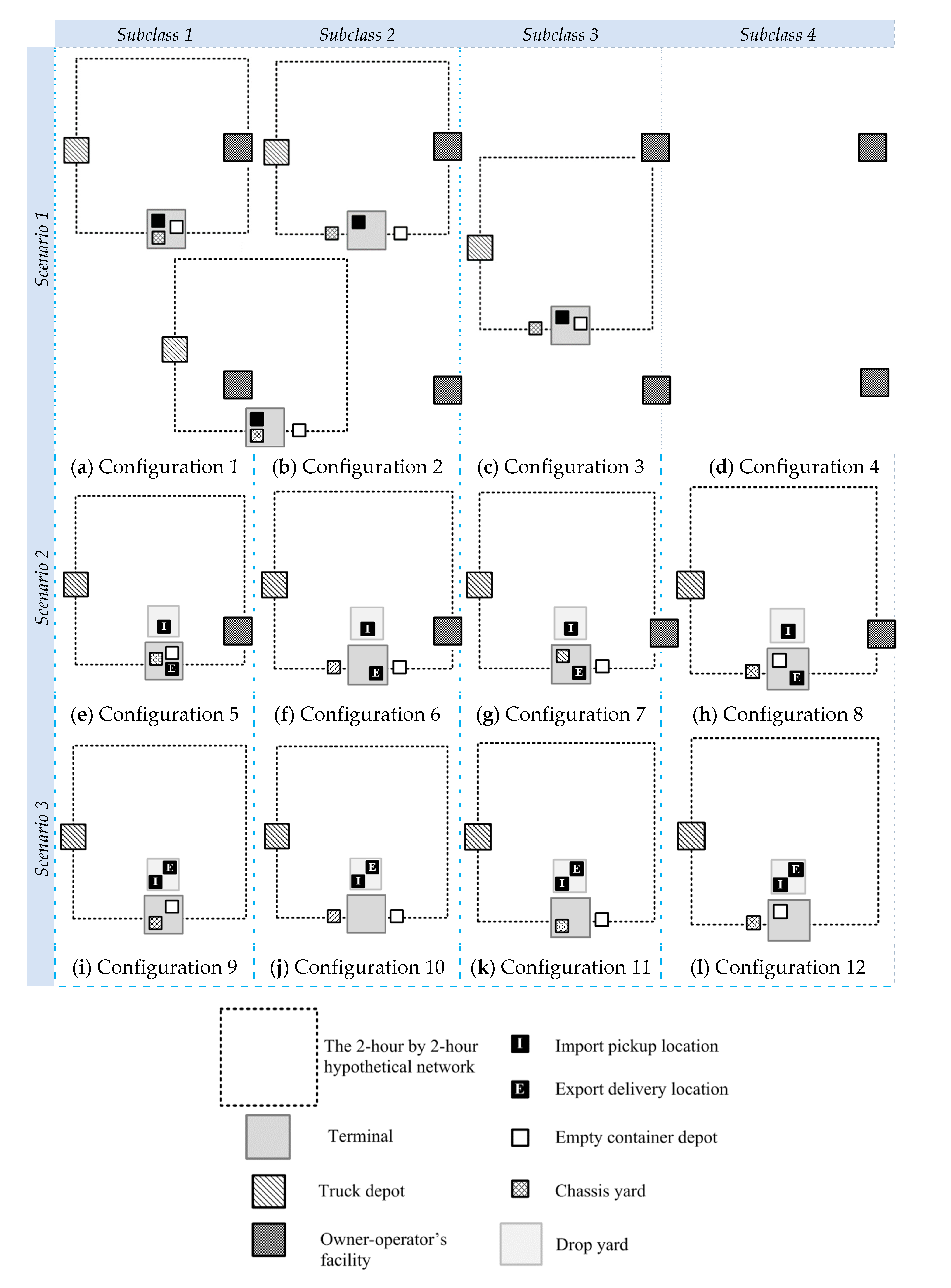
Based on the location of the chassis yard, empty container depot, import pickup, and export delivery, 12 configurations were considered as shown in Figure 4. Note that Configurations 1 to 4 (Figure 4a–d) are associated with Scenario 1, Configurations 5 to 8 (Figure 4e–h) are associated with Scenario 2, and Configurations 9 to 12 (Figure 4i–l) are associated with Scenario 3. An experimental design was set up to study the effect of the aforementioned scenarios on drayage operation time. One type of experimental design is factorial experimental design (FED). In FED, first, a set of “factors” is selected which consists of the variables that are chosen to be studied. Then, these factors are systematically set to predefined discrete values, known as “levels.” In FED, combinations of all levels of factors are considered, and then the effect of each combination on the output is studied.
In this study, the factors considered, and their levels are as follows.
  • Problem size in terms of number of job nodes (PS)
  • Levels: (1) 60, and (2) 100
  • Scenario (S)
  • Levels: (1) Scenario 1, (2) Scenario 2, and (3) Scenario 3
  • Empty container depot location (ECL)
  • Levels: (1) inside the terminal (ONEC), and (2) outside the terminal (OFFEC)
  • Chassis yard location (CHSS)
  • Levels: (1) inside the terminal (ONTY), (2) outside the terminal in (OFFTY)
  • Percent of job nodes: % of empty container delivery nodes, % of loaded container delivery nodes, % of empty container pickup nodes, % of loaded container pickup nodes (PJN):
  • Levels: (1) 25:25:25:25, and (2) 15:35:35:15
The combination of factors and levels result in a 2 × 3 × 2 × 2 × 2 factorial design which yields a total of 48 problem classes. For each problem class, three instances are randomly generated which yields 144 experiments. The 25:25:25:25 is equivalent to the typical percent of job nodes at the Port of Oakland’s terminal gate transactions, and the 15:35:35:15 is equivalent to the typical percent of job nodes at Port of Long Beach’s terminal gate transactions, based on available data.
To facilitate the presentation of the results, the combination of factors (3 and 4) and their levels are grouped into subclasses, as outlined below.
Subclass 1. ONEC and ONTY (Configurations 1, 5 and 9 shown in Figure 4)
Subclass 2. OFFEC and OFFTY (Configurations 2, 6 and 10 shown in Figure 4)
Subclass 3. OFFEC and ONTY (Configurations 3, 7 and 11 shown in Figure 4)
Subclass 4. ONEC and OFFTY (Configurations 4, 8 and 12 shown in Figure 4)
The subclasses are illustrated in Figure 4 by the dashed blue lines. Note that for subclass 1, both the chassis yard and empty container depot are located inside the marine terminal. For subclass 2, both are located outside the marine terminal. For subclass 3, the chassis yard is located inside the marine terminal and the empty container depot is located outside. Lastly, for subclass 4, the chassis yard is located outside the marine terminal and the empty container depot is located inside.

4.2. Experimental Results and Discussion

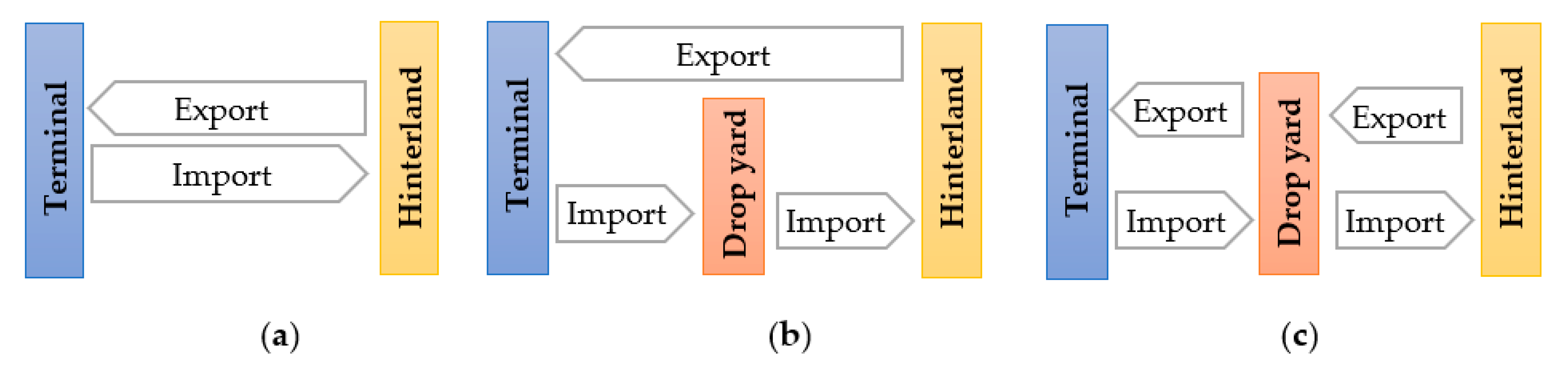
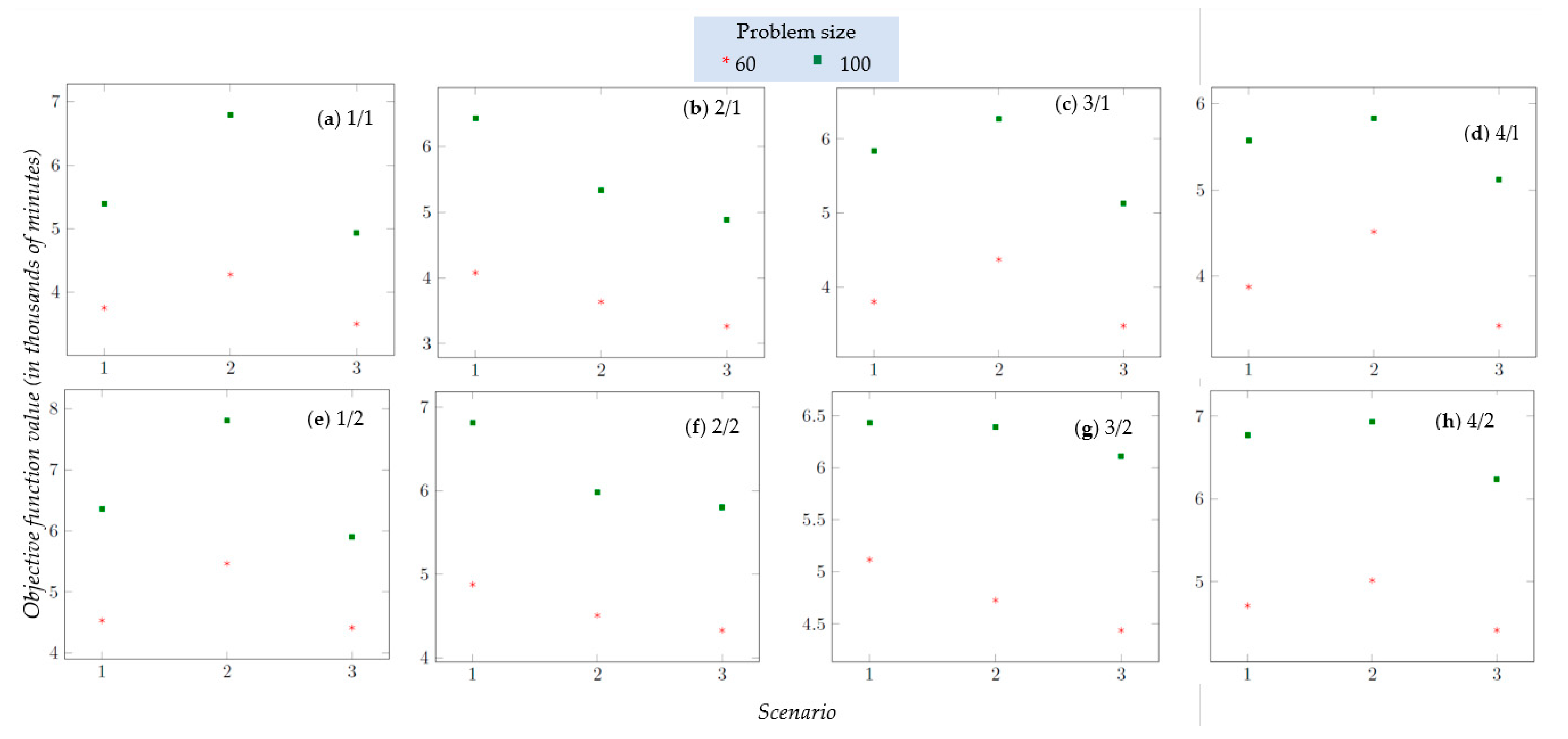
Figure 5 shows the average drayage operation time for all classes. The results are divided into eight groups (denoted as a-h) by the subclasses and percent of job nodes. The subclass and percent of job nodes are shown in the upper right-hand corner of each box. For example, in the group a, the value “1/1” denotes Subclass 1 and percent of job nodes level 1. The asterisks on each box denote the average drayage operation time for classes with 60 job nodes, and the squares on each box denote classes with 100 job nodes. To understand the impact of second-tier facilities, in the following, it may be helpful to recall that Scenario 1 represents the traditional drayage practice where the import and export operations take place inside the marine terminal. Scenario 2 and 3 represent new practices. Import operations take place at the drop yard in Scenario 2, and both import and export operations take place at the drop yard in Scenario 3. Figure 5a–d show the results of classes where the percent of job nodes is equal to 25:25:25:25. Figure 5e–h show the results of classes where the percent of job nodes is equal to 15:35:35:15. Based on the experimental results for all the subclasses in Scenario 1, Subclass 1 has the lowest drayage operation time. Based on the experimental results for all the subclasses in Scenario 2, Subclass 2 has the lowest drayage operation time. Similarly, based on the experimental results for all the subclasses in Scenario 3, Subclass 2 has the lowest drayage operation time. Overall, the results from all sets of experiments showed that Scenario 3 with Subclass 2 has the lowest drayage operation time.
Table 5 and Table 6 show the relative ranking of traditional and new practices in placing import pickup and export delivery locations (i.e., scenarios) based on drayage operation time. It may be helpful to recall that in the traditional practice both import pickup and export delivery locations are inside the terminal, and in the new practices, either only import pickup location is at an off-terminal drop yard and export delivery location is inside the terminal, or both import pickup and export delivery locations are at an off-terminal drop yard. Rankings are provided in different configurations of chassis yard and empty container depot locations (i.e., inside/on-terminal or outside/off-terminal). Table 5 and Table 6 show the results of experiments where the percent of job nodes are 25:25:25:25 and 15:35:35:15, respectively.
Results show that the new practice where both import pickup and export delivery locations are at an off-terminal drop yard has the lowest drayage operation time in all configurations of chassis yard and empty container depot locations. From these results, it can be concluded that by moving the locations of both import pickup and export delivery from inside
The container terminal to a location outside the terminal, the efficiency of drayage operation would increase. The reason is that the drop yard has shorter queues and shorter turn times compared to the marine terminal, which leads to net improvement in drayage operation efficiency.
Comparing the results of the traditional practice against the new practice, where only export delivery location is inside the terminal and import pickup location is outside the terminal, indicated that depending on the percent of job nodes as well as the locations of chassis yard and empty container depot, either of these two practices have the second-lowest drayage operation time. When there are an equal number of empty container delivery, loaded container delivery, empty container pickup and loaded container pickup requests (i.e., the percent of job nodes is 25:25:25:25), traditional practice where both import pickup and export delivery locations are inside the terminal has the second-lowest drayage operation time with configurations where empty container depot and/or chassis yard are located inside the terminal. The reason is that drayage operation efficiency will increase by utilizing double moves inside the terminal in the traditional practice. However, when both empty container depot and chassis yard are located outside the terminal trucks can make fewer double moves inside the terminal. As a result, the new practice where only import pickup location is at an off-terminal drop yard, with shorter queues and shorter turn times compared to the marine terminal, becomes the practice with second-lowest drayage operation time where both chassis yard and empty container location are outside the terminal.
When the percent of job nodes is 15:35:35:15 (i.e., 15% of empty container delivery nodes, 35% of loaded container delivery nodes, 35% of empty container pickup nodes, 15% of loaded container pickup nodes), the number of customers with empty container pickup and loaded container delivery requests are higher than the number of customers with empty container delivery and loaded container pickup requests. As a result, the locations of empty container depot and import pickup play a critical role in the efficiency of drayage operation (i.e., whether or not both are inside the terminal). Traditional practice where both import pickup and export delivery locations are inside the terminal has the second-lowest operation time with the configurations in which the empty container depot is inside the terminal. The reason is that in this practice trucks can make double moves inside the marine terminal, picking up import containers after delivering empty containers (the percentage of both is 35%) which improves drayage efficiency and makes this scenario more efficient where empty containers are located inside the terminal. The new practice where only import pickup location is at an off-terminal drop yard and export delivery location is inside the terminal has the second-lowest operation time in configurations where empty container depot is located outside the terminal. The reason is that in this practice, import pickup location is outside the terminal and trucks can make less double moves inside the terminal. Instead, the shorter queues and shorter turn times at the drop yard and the off-terminal empty container depot play a critical role in the efficiency of drayage operation in this scenario and make it more efficient in the configurations where the empty container depot is located outside the terminal.
Table 7 shows the most efficient locations for empty container depot and chassis yard in traditional and new practices of placing import pickup and export delivery locations in the U.S. When both import pickup and export delivery locations are inside the terminal, the most efficient locations for empty container depot and chassis yard are inside the terminal. The reason is that with chassis, empty containers, import containers and export containers being stored at the terminal, trucks can drop off a chassis/empty container/loaded container and then pick up a chassis/empty container/loaded container on the same trip. When import pickup and/or export delivery locations are at drop yard, the most efficient locations for the chassis yard and empty container depot are outside the terminal. The reason is that when import and/or export containers are located outside the terminal, the truck cannot make double moves for import pickup and/or export delivery inside the terminal. Instead, by locating both empty container depot and chassis yard outside the terminal, drayage operation efficiency will increase as these facilities have a shorter queue and shorter turn times compared to the marine terminal. The results suggest that there is a logic to facility grouping. The chassis pools and container depots are most efficiently located with the last mile deliveries and pickups. If the driver who will deliver the import container to the consignee comes to the marine terminal, then the chassis and container depots should be there too. However, if that driver picks up the import container at an off-terminal drop yard, the empty container depot and chassis yard should be at the off-terminal locations as well.
The results show, in the traditional practice, by moving the location of empty container depot to a location outside the terminal, drayage operation time increased by 6% on average. Similarly, by moving the location of chassis to a location outside the terminal, drayage operation time increase 4% on average. When both empty container depot and chassis yard are moved to outside the terminal drayage operation time increased by 11% on average. Additionally, for the scenario in which the drop yard is used for import only, drayage operation time increased by 21% on average where both chassis yard and empty container are located inside the terminal. Drayage operation time increased by 9% on average where chassis yard is located inside the terminal and empty container are located outside the terminal. Additionally, drayage operation time increased by 12% where chassis yard is located outside the terminal and empty container depot is located inside the terminal. However, when both chassis yard and empty container depot are located outside the terminal drayage operation time decreased by 2%.
Finally, the results show that in all configurations of empty container depot and chassis yard locations, moving both import pickup and export delivery locations to outside the terminal will improve drayage operation time between 4% and 9% on average.

5. Conclusions

This paper builds on the authors’ previously drayage scheduling model to study the impact of second-tier facilities on drayage operation time. This model is modified by incorporating these features: (1) trucks do not have to wait at customers’ locations during the import unloading and export loading operations; (2) drayage operations can include a drop yard (i.e., second-tier facility) for picking up or/and dropping off loaded containers outside the marine container terminal; and (3) a customer is allowed to request any of the following jobs: pick up an empty container, pick up a loaded container, drop off an empty container, or drop off a loaded container. The results indicated that: (1) moving the location of both import pickup and export delivery from inside the marine container terminal to a location outside the terminal could increase the efficiency of drayage operation; the key factors in these drayage efficiency gains are the shorter queues and truck turn times that are typical of second-tier facilities; (2) when import pickup and export delivery take place inside the marine container terminal, the most efficient location for the chassis yard and empty container depot is inside the terminal; and (3) when the location of import pickup and/or export delivery are outside the terminal, the most efficient location for the chassis yard and empty container depot is also outside the terminal.
Most second-tier facilities have been created to provide additional capacity for marine container terminals or as buffers to reconcile the preferred delivery times of importers with the available gate hours of marine terminals. This study’s findings suggest that these facilities could also yield operational savings provided they have shorter queuing and turn time as compared to marine container terminals. That is, port authorities and terminal operators must ensure that the second-tier facilities have significantly lower turn time compared to the container terminal. For example, actual operational data from the PoLB’s STOR show that its turn time is 12 to 17 min compared to 50 min or longer for single transactions at one of its container terminals. The other key takeaway for port authorities and terminal operators from this study is that their terminal and facilities must be set up to facilitate double moves; otherwise, truckers will end up making two separate moves which will negate the benefits of second-tier facilities. A reason why STOR has worked out well for the PoLB is because 80% to 90% of the moves at STOR are double moves. The final takeaway from this study is that it is possible for North American marine container terminals to evolve from self-contained entities into multi-tier systems. Thus, city officials and transportation planners in states with marine container terminals should be aware of this possibility when creating policies and plans for their regional communities.
This study has a few assumptions that can be extended in future research. The operation times and travel times were assumed to be deterministic. To make the model reflect realistic conditions, a stochastic model can be formulated to account for uncertainty in operation and travel times. To accomplish this, actual operational data and travel time data are needed to develop best fit distributions. Along the line of uncertainty in travel time, disruptions such as those caused by traffic accidents can also be incorporated into the stochastic model. To do this, a crash frequency model will need to developed using crash data. Additionally, needed are the durations of the accidents. Lastly, the study’s findings will be more generalizable if it uses an actual intermodal freight network instead of a hypothetical one. If terminal data can be made available, it would allow for the validation of certain performance measures such as number of moves at a facility and total drayage time.

Author Contributions

The authors confirm contribution to the paper as follows: study conception and design: S.S., D.S., N.H. and F.H.; analysis and interpretation of results: S.S. and N.H.; draft manuscript preparation: S.S., D.S., N.H. and F.H. All authors reviewed the results and approved the final version of the manuscript. All authors have read and agreed to the published version of the manuscript.

Funding

This research was funded by the National Science Foundation under Grant number 1100227, and the APC was funded by the University of South Carolina.

Data Availability Statement

The data that support the findings of this study are available from the corresponding author, NH, upon reasonable request.

Conflicts of Interest

The authors declared no potential conflict of interest with respect to the research, authorship, and/or publication of this article.

References

  1. Port of Long Beach. STOR Yard Gives Cargo Some Space. Available online: https://polb.com/port-info/news-and-press/stor-yard-gives-cargo-some-space-12-17-2020/ (accessed on 14 September 2022).
  2. Wang, X.; Regan, A.C. Local truckload pickup and delivery with hard time window constraints. Transp. Res.-Part B 2002, 36, 97–112. [Google Scholar] [CrossRef]
  3. Ileri, Y.; Bazaraa, M.; Gifford, T.; Nemhauser, G.; Sokol, J.; Wikum, E. An optimization approach for planning daily drayage operations. Cent. Eur. J. Oper. Res. 2006, 14, 141–156. [Google Scholar] [CrossRef]
  4. Imai, A.; Nishimura, E.; Current, J. A Lagrangian relaxation-based heuristic for the vehicle routing with full container load. Eur. J. Oper. Res. 2007, 176, 87–105. [Google Scholar] [CrossRef]
  5. Caris, A.; Janssens, G.K. A local search heuristic for the pre-and end-haulage of intermodal container terminals. Comput. Oper. Res. 2009, 36, 2763–2772. [Google Scholar] [CrossRef]
  6. Nossack, J.; Pesch, E. A truck scheduling problem arising in intermodal container transportation. Eur. J. Oper. Res. 2013, 230, 666–680. [Google Scholar] [CrossRef]
  7. Zhang, R.; Yun, W.Y.; Moon, I. A reactive tabu search algorithm for the multi-depot container truck transportation problem. Transp. Res. Part E 2009, 45, 904–914. [Google Scholar] [CrossRef]
  8. Zhang, R.; Yun, W.Y.; Kopfer, H. Heuristic-based truck scheduling for inland container transportation. OR Spectr. 2010, 32, 787–808. [Google Scholar] [CrossRef]
  9. Zhang, G.; Smilowitz, K.; Erera, A. Dynamic planning for urban drayage operations. Transp. Res.-Part E 2011, 47, 764–777. [Google Scholar] [CrossRef]
  10. Braekers, K.; Caris, A.; Janssens, G.K. Integrated planning of loaded and empty container movements. OR Spectr. 2013, 35, 457–478. [Google Scholar] [CrossRef]
  11. Braekers, K.; Caris, A.; Janssens, G.K. Bi-objective optimization of drayage operations in the service area of intermodal terminals. Transp. Res.-Part E 2014, 65, 50–69. [Google Scholar] [CrossRef]
  12. Shiri, S.; Huynh, N. Assessment of US chassis supply models on drayage productivity and air emissions. Transp. Res.-Part D 2017, 61, 174–203. [Google Scholar] [CrossRef]
  13. Vidović, M.; Nikolić, M.; Popović, D. Two mathematical formulations for the containers drayage problem with time windows. Int. J. Bus. Sci. Appl. Manag. 2012, 7, 23–32. [Google Scholar]
  14. Vidović, M.; Popović, D.; Ratković, B.; Radivojević, G. Generalized mixed integer and VNS heuristic approach to solving the multisize containers drayage problem. Int. Trans. Oper. Res. 2016, 24, 583–614. [Google Scholar] [CrossRef]
  15. Popović, D.; Vidović, M.; Nikolić, M. The variable neighborhood search heuristic for the containers drayage problem with time windows. Soft Comput. Ind. Appl. 2014, 223, 351–364. [Google Scholar]
  16. Zhang, R.; Yun, W.Y.; Kopfer, H. Multi-size container transportation by truck: Modeling and optimization. Flex. Serv. Manuf. J. 2015, 27, 403–430. [Google Scholar] [CrossRef]
  17. Funke, J.; Kopfer, H. A model for a multi-size inland container transportation problem. Transp. Res.-Part E Logist. Transp. Rev. 2016, 89, 70–85. [Google Scholar] [CrossRef]
  18. Namboothiri, R.; Erera, A.L. Planning local container drayage operations given a port access appointment system. Transp. Res.-Part E 2008, 44, 185–202. [Google Scholar] [CrossRef]
  19. Shiri, S.; Huynh, N. Optimization of drayage operations with time-window constraints. Int. J. Prod. Econ. 2016, 176, 7–20. [Google Scholar] [CrossRef]
  20. Cheung, R.K.; Hange, D.D. A time-window sliding procedure for driver-task assignment with random service times. IIE Trans. 2003, 35, 433–444. [Google Scholar] [CrossRef]
  21. Cheung, R.K.; Hang, D.D.; Shi, N. A labeling method for dynamic driv-er-task assignment with uncertain task durations. Oper. Res. Lett. 2005, 33, 411–420. [Google Scholar] [CrossRef]
  22. Shiri, S.; Ng, M.; Huynh, N. Distribution-Free Scheduling of Drayage Operation under Uncertainty. In Proceedings of the 97th Annual Meeting of the Transportation Research Board, Washington DC, USA, 7–11 January 2018. [Google Scholar]
  23. Sterzik, S.; Kopfer, H.; Yun, W.Y. Reducing hinterland transportation costs through container sharing. Flex. Serv. Manuf. J. 2015, 27, 382–402. [Google Scholar] [CrossRef]
  24. Wang, X.; Kopfer, H. Rolling horizon planning for a dynamic collaborative routing problem with full-truckload pickup and delivery requests. Flex. Serv. Manuf. J. 2015, 27, 509–533. [Google Scholar] [CrossRef]
  25. Lei, T.L.; Church, R.L. Locating short-term empty-container storage facilities to support port operations: A user optimal approach. Transp. Res.–Part E 2011, 47, 738–754. [Google Scholar] [CrossRef]
  26. Huynh, N. Methodologies for Reducing Truck Turn Time at Marine Container Terminals. Ph.D. Thesis, The University of Texas at Austin, Austin, TX, USA, 2005. [Google Scholar]
  27. NCFRP Report 20. Guidebook for Assessing Evolving International Container Chassis Supply Models; Transportation Research Board of the National Academies: Washington, DC, USA, 2012. [Google Scholar]
Figure 1. Newly established drop yard at the Port of Long Beach.
Logistics 06 00068 g001
Figure 2. Drayage practice: (a) traditional drayage process; (b) drayage with drop yard used for imports; (c) drayage with drop yard used for both exports and imports.
Logistics 06 00068 g002
Figure 3. Flowchart of developed solution methodology.
Logistics 06 00068 g003
Figure 4. Location of the marine terminal and second-tier facilities considered in experiments.
Logistics 06 00068 g004
Figure 5. Average drayage operation time by scenarios according to subclass/level of percent of job nodes.
Logistics 06 00068 g005
Table 1. Transfer Time on Arc (i,j) for Scenario 1.
TTijTo Node j
ND/ND’NEP/NLPNEDNLD
From nodeiND/ND’-T(TDi,CHY) + GTCHY + PCH + T(CHY,CLj) + GTCLT(TDi,CHY) + GTCHY + PCH + T(CHY,ECD) + GTECD + PEC + T(ECD,CLj) + GTCLT(TDi,CHY) + GTCHY + PCH + T(CHY,T) + GTT + PLC + T(T,CLj) + GTCL
NEPT(CLi,ECD) + GTECD + DEC + (ECD,CHY) + GTCHY + DCH + T(CHY,TDj)IFS(i) = S(j) 1 T(CLi,ECD) + GTECD + DEC + T(ECD,CLj) + GTCL ELSE T(CLi,ECD) + GTECD + DEC + T(ECD,CHY) + GTCHY + SCH + T(CHY, CLj) + GTCLIFS(i) = S(j) T(CLi,CLj) + GTCL ELSE T(CLi,ECD) + GTECD + DEC + T(ECD,CHY) + GTCHY + SCH + T(CHY,ECD) + GTECD + PEC + T(ECD, CLj) + GTCLIFS(i) = S(j) T(CLi,ECD) + GTECD + DEC + T(ECD,T) + GTT + PLC + T(T, CLj) + GTCL ELSE T(CLi,ECD) + GTECD + DEC + T(ECD,CHY) + GTCHY + SCH + T(CHY,T) + GTT + PLC + T(T, CLj) + GTCL
NLPT(CLi,T) + GTT + DLC + T(T,CHY) + GTCHY + DCH + T(CHY,TDj)IFS(i) = S(j) T(CLi,T) + GTT + DLC + T(T,CLj) ELSE T(CLi,T) + GTT + DLC + T(T,CHY) + GTCHY + SCH + T(CHY,CLj) + GTCLIFS(i) = S(j) T(CLi,T) + GTT + DLC + T(T,ECD) + PEC + T(ECD,CLj) + GTCL ELSE T(CLi,T) + GTT + DLC + T(T,CHY) + GTCHY + SCH + T(CHY,ECD) + GTECD + PEC + T(ECD, CLj) + GTCLIFS(i) = S(j) T(CLi,T) + GTT + DLC + PLC + T(T,CLj) + GTCL ELSE T(CLi,T) + GTT + DLC + T(T,CHY) + GTCHY + SCH + T(CHY,T) + GTT + PLC + T(T,CLj) + GTCL
NED/NLDT(CLi,CHY) + GTCHY + DCH + T(CHY,TDj)IFS(i) = S(j) T(CLi,CLj) + GTCL ELSE T(CLi,CHY) + GTCHY + SCH + T(CHY,CLj) + GTCLIFS(i) = S(j) T(CLi,ECD) + GTECD + PEC + T(ECD, CLj) + GTCL ELSE T(CLi,CHY) + GTCHY + SCH + T(CHY,ECD) + GTECD + PEC + T(ECD, CLj) + GTCLIFS(i) = S(j) T(CLi,T) + GTT + PLC + T(T, CLj) + GTCL ELSE T(CLi,CHY) + GTCHY + SCH +T(CHY,T) + GTT + PLC + T(T,CLj) + GTCL
1 If chassis and/or containers can be used for job j after job i.
Table 2. Transfer Time on Arc (i,j) for Scenario 2.
TTijTo Node j
ND /ND’NEP/NLPNEDNLD
From nodeiND/ND’-T(TDi,CHY) + GTCHY + PCH + T(CHY,CLj) + GTCLT(TDi,CHY) + GTCHY + PCH + T(CHY,ECD) + GTECD + PEC + T(ECD,CLj) + GTCLT(TDi,DY) + GTDY + PLC + T(DY,CLj) + GTCL
NEPT(CLi,ECD) + GTECD + DEC + (ECD,CHY) + GTCHY + DCH + T(CHY,TDj)IFS(i) = S(j) 1 T(CLi,ECD) + GTECD + DEC + T(ECD,CLj) + GTCL ELSE T(CLi,ECD) + GTECD + DEC + T(ECD,CHY) + GTCHY + SCH + T(CHY, CLj) + GTCLIFS(i) = S(j) T(CLi,CLj) + GTCL ELSE T(CLi,ECD) + GTECD + DEC + T(ECD,CHY) + GTCHY + SCH + T(CHY,ECD) + GTECD + PEC + T(ECD, CLj) + GTCLT(CLi,ECD) + GTECD + DEC + T(ECD,CHY) + GTCHY + DCH + T(CHY,DY) + GTDY + PLC + T(DY,CLj) + GTCL
NLPT(CLi,T) + GTT + DLC + T(T,CHY) + GTCHY + DCH + T(CHY,TDj)IFS(i) = S(j) T(CLi,T) + GTT + DLC + T(T,CLj) + GTCL ELSE T(CLi,T) + GTT + DLC + T(T,CHY) + GTCHY + SCH + T(CHY,CLj) + GTCLIFS(i) = S(j) T(CLi,T) + GTT + DLC + T(T,ECD) + GTECD + PEC + T(ECD,CLj) + GTCL ELSE T(CLi,T) + GTT + DLC + T(T,CHY) + GTCHY + SCH + T(CHY,ECD) + GTECD + PEC + T(ECD, CLj) + GTCLT(CLi,T) + GTT + DLC + T(T,CHY) + GTCHY + DCH + T(CHY,DY) + GTDY + PLC + T(DY,CLj) + GTCL
NED/NLDT(CLi,CHY) + GTCHY + DCH + T(CHY,TDj)IFS(i) = S(j) T(CLi,CLj) + GTCL ELSE T(CLi,CHY) + GTCHY + SCH + T(CHY,CLj) + GTCLIFS(i) = S(j) T(CLi,ECD) + GTECD + PEC + T(ECD, CLj) + GTCL ELSE T(CLi,CHY) + GTCHY + SCH + T(CHY,ECD) + GTECD + PEC + T(ECD, CLj) + GTCLT(CLi,CHY) + GTCHY + DCH + T(CHY,DY) + GTDY + PLC + T(DY,CLj) + GTCL
1 If chassis and/or containers can be used for job j after job i.
Table 3. Transfer Time on Arc (i,j) for Scenario 3.
TTijTo Node j
ND /ND’NEP/NLPNEDNLD
From nodeiND/ND’-T(TDi,CHY) + GTCHY + PCH + T(CHY,CLj) + GTCLT(TDi,CHY) + GTCHY + PCH + T(CHY,ECD) + GTECD + PEC + T(ECD,CLj) + GTCLT(TDi,DY) + GTDY + PLC + T(DY,CLj) + GTCL
NEPT(CLi,ECD) + GTECD + DEC + (ECD,CHY) + GTCHY + DCH + T(CHY,TDj)IFS(i) = S(j) 1 T(CLi,ECD) + GTECD + DEC + T(ECD,CLj) + GTCL ELSE T(CLi,ECD) + GTECD + DEC + T(ECD,CHY) + GTCHY + SCH + T(CHY, CLj) + GTCLIFS(i) = S(j) T(CLi,CLj) + GTCL ELSE T(CLi,ECD) + GTECD + DEC + T(ECD,CHY) + GTCHY + SCH + T(CHY,ECD) + GTECD + PEC + T(ECD, CLj) + GTCLT(CLi,ECD) + GTECD + DEC + T(ECD,CHY) + GTCHY + DCH + T(CHY,DY) + GTDY + PLC + T(DY,CLj) + GTCL
NLPT(CLi,DY) + GTDY + DLC + T(DY,TDj)T(CLi,DY) + GTDY + DLC + T(DY,CHY) + GTCHY + PCH + T(CHY,CLj) + GTCLT(CLi,DY) + GTDY + DLC + T(DY,CHY) + GTCHY + PCH + T(CHY,ECD) + GTECD + PEC + T(ECD,CLj) + GTCLT(CLi,DY) + GTDY + DLC + PLC + T(DY,CLj) + GTCL
NED/NLDT(CLi,CHY) + GTCHY + DCH + T(CHY,TDj)IFS(i) = S(j) T(CLi,CLj) + GTCL ELSE T(CLi,CHY) + GTCHY + SCH + T(CHY,CLj) + GTCLIFS(i) = S(j) T(CLi,ECD) + GTECD + PEC + T(ECD, CLj) + GTCL ELSE T(CLi,CHY) + GTCHY + SCH + T(CHY,ECD) + GTECD + PEC + T(ECD, CLj) + GTCLT(CLi,CHY) + GTCHY + DCH + T(CHY,DY) + GTDY + PLC + T(DY,CLj) + GTCL
1 If chassis and/or containers can be used for job j after job i.
Table 4. Transaction Times at T, CHY, ECD, DY, and CL.
Transaction TypeTime (Min)
TCHYECDDYCL
Gate queueing time305555
Time to pick up a loaded container30NANA105
Time to drop off a loaded container20NANA105
Time to pick up an empty container15NA10NA5
Time to drop off an empty container10NA10NA5
Swapping chassis2515NANANA
Time to pick up chassis1510NANANA
Time to drop off chassis105NANANA
Table 5. The relative ranking of traditional and new practices in placing import pickup and export delivery locations (i.e., scenarios) based on drayage operation time where percent of job nodes is 25:25:25:25.
On-Terminal Import Pickup and Export Delivery LocationsOff-Terminal Import Pickup and On-Terminal Export Delivery LocationsOff-Terminal Import Pickup and Export Delivery Locations
Chassis yardOn-terminalEmpty container depotOn-terminalSecond-lowestHighestLowest
Off-terminalSecond-lowestHighestLowest
Off-terminalEmpty container depotOn-terminalSecond-lowestHighestLowest
Off-terminalHighestSecond-lowestLowest
Table 6. The relative ranking of traditional and new practices in placing import pickup and export delivery locations (i.e., scenarios) based on drayage operation time where percent of job nodes is 15:35:35:15.
On-Terminal Import Pickup and Export Delivery LocationsOff-Terminal Import Pickup and On-Terminal Export Delivery LocationsOff-Terminal Import Pickup and Export Delivery Locations
Chassis yardOn-terminalEmpty container depotOn-terminalSecond-lowestHighestLowest
Off-terminalHighestSecond-lowestLowest
Off-terminalEmpty container depotOn-terminalSecond-lowestHighestLowest
Off-terminalHighestSecond-lowestLowest
Table 7. The best locations for placing empty container depot and chassis yard according to locations of import pickup and export delivery.
On-Terminal Import Pickup and Export Delivery LocationsOff-Terminal Import Pickup and On-Terminal Export Delivery LocationsOff-Terminal Import Pickup and Export Delivery Locations
Empty container depotOn-terminalOff-terminalOff-terminal
Chassis yardOn-terminalOff-terminalOff-terminal
Publisher’s Note: MDPI stays neutral with regard to jurisdictional claims in published maps and institutional affiliations.

