Abstract
Conventional wavefront sensors face challenges when detecting frequency-domain information. In this study, we developed a high-precision, and fast multi-spectral wavefront detection technique based on neural networks. Using an etalon and a diffractive optical element for spectral encoding, the measured pulses were spatially dispersed onto the sub-apertures of the Shack-Hartmann wavefront sensor (SHWFS). We employed a neural network model as the decoder to synchronously calculate the multi-spectral wavefront aberrations. Numerical simulation results demonstrate that the average calculation time is 21.38 ms, with a root mean squared (RMS) wavefront residual error of approximately 0.010 μm for 4-wavelength, 21st-order Zernike coefficients. By comparison, the conventional modal-based algorithm achieves an average calculation time of 102.98 ms and wavefront residuals of 0.090 μm. Remarkably, for 10-wavelength analysis, traditional centroid algorithms fail; this approach maintains high simulation accuracy with the RMS wavefront residual error below 0.016 μm. The proposed approach significantly enhances the measurement capabilities of SHWFS in multi-spectral and single-shot wavefront detection, particularly for single-shot spatio-temporal characterization in ultra-intense and ultra-short laser systems.
1. Introduction
Wavefront aberrations generated by the amplification and transmission processes significantly affect the focused intensity and output performance of ultra-intense and ultra-short laser systems. To improve the intensity of the focal spot, adaptive optics (AO) systems are commonly used to measure, control, and correct wavefront aberrations [1,2,3]. As an important tool for wavefront detection in AO systems, the Shack–Hartmann wavefront sensor (SHWFS) utilizes the centroid displacement of microlens arrays to reconstruct the incident wavefront [4,5] and has been widely applied in high-filed lasers [2], astronomical systems [6], ophthalmology [7], and bioimaging [8]. Recent progress has included a plug-and-play conjugate AO module [9], high-speed AO systems for stabilizing high-intensity laser facilities [10], and a computational scattering-matrix method for digital correction [11].
In petawatt-class ultra-intense and ultra-short laser systems, the stretcher, compressor, and beam expander facilities introduce spatio-temporal coupling (STC) effects such as pulse-front tilt (PFT), pulse-front curvature (PFC), and complex spatio-temporal coupling distortion, which are characterized by the spectral properties of the laser pulses with respect to the spatial position [12,13,14,15]. STC effects can increase the focal spot size and the focus pulse duration, which degrade focused intensities and peak power density, ultimately degrading output performance [16,17,18]. Scanning spatio-temporal detection techniques represent a major direction for international development [12]. However, petawatt-class ultra-intense and ultra-short lasers operate at low repetition rates or even in single-shot mode [19,20], which limits the applicability of these scanning techniques. Furthermore, conventional wavefront sensors, such as SHWFS and the four-wave lateral shearing interferometer (SID4), cannot measure the wavefront aberrations of individual spectral components within broadband pulses [21,22,23]. This restricts their application to petawatt-class laser systems that exhibit STC effects. Frequency-resolved wavefront sensing methods, which integrate wavefront sensors with filtering, encoding, and other technologies, have been developed to enable single-shot measurements [24,25,26]. However, these methods still face challenges regarding the limited number of measurable spectral channels and complex optical setups. Therefore, expanding the frequency-domain measurement capabilities of traditional wavefront sensors and developing multi-spectral and single-shot wavefront sensing techniques are essential for advancing high-power laser system diagnostics.
In recent years, convolutional neural networks (CNNs) have emerged as the crucial algorithms in deep learning (DL) and have been introduced in many optical imaging fields owing to their significant role in solving a variety of optical image processing problems, such as digital holography [27], super-resolution microscopy [28] and computational imaging [29]. In AO systems, CNNs have also been successfully applied in wavefront sensing and phase recovery. Hu et al. constructed a learning-based SHWFS model that could directly detect higher-order Zernike coefficients from the output pattern of the SHWFS with high accuracy and detection speed [30,31]. He et al. utilized the Residual Shrinkage Network (ResNet) to accurately reconstruct 88-order Zernike coefficients with fewer SHWFS sub-apertures [32]. Zhao et al. proposed a CNN-based centroid-prediction method for sub-apertures that are weak or missing from the SHWFS [33]. Ziemann et al. employed CNNs to directly reconstruct high-resolution wavefronts from event-based sensor data, achieving a 73% increase in reconstruction fidelity compared with existing methods [34]. Qiao et al. proposed a novel space-frequency encoding network (SFE-Net) that can directly estimate aberrated PSFs from biological images, enabling fast optical aberration estimation with high accuracy [35]. The above studies have shown that deep learning can significantly improve wavefront detection ability in AO systems. In particular, it can improve the measurement accuracy and application performance of SHWFS. Based on this research, we developed an end-to-end, multi-spectral, single-shot wavefront detection technique that combines optical coding with a neural network (NN) to extend the frequency-domain detection capability of the SHWFS [36,37].
To address the inability of an SHWFS to perform frequency-domain detection, we developed a simple, high-precision, and fast multi-spectral wavefront detection technique based on neural networks. This approach comprises two parts: diffractive Hartmann wavefront sensing for hardware measurement and neural network-based phase reconstruction. This approach overcomes the problem of overlapping spectral components, which lead to incorrect centroid calculations, and the spectral resolution can be improved by increasing the size of the individual sub-aperture.
The rest of the paper is organized as follows: Section 2 describes the system design and calculates the parameters of the required optical components. The structure of the neural network model and the form of the dataset are also presented. Section 3 presents the numerical simulation results and compares their performance with those of conventional centroid algorithms. Finally, the conclusions of this study are presented in Section 4.
2. Methods
In this section, we introduce the multi-spectral wavefront measurement scheme and setup, calculate the optical system parameters, and present the neural network architecture and dataset configuration for model training.
2.1. System Design
The design of the optical measurement module is illustrated in Figure 1. It comprises a spectral phase meter, spectral encoder, spectrometer, and wavefront measurement sensor. To assist in the frequency-domain characterization, a portion of the beam was separated and directed to a spectral phase meter (e.g., Wizzler) to measure the initial spectrum and spectral phase of the measured pulse. Subsequently, an etalon and a diffraction grating were employed for spectral encoding. The etalon spatially dispersed the incident pulse into discrete spectral bands, whereas the diffraction grating (used in our numerical simulations) introduced a frequency-dependent dispersion. This dispersion laterally separated the spectral components of the pulse within each SHWFS sub-aperture, appearing as additional tilt errors. Finally, a spectrometer was employed to measure the spectral components encoded by the etalon of the zero-order signal, whereas an SHWFS with a large sub-aperture microlens was used to detect the first-order multi-spectral diffraction signals. Following data acquisition, a trained neural network processed the spectrally encoded SHWFS array pattern to predict the multispectral Zernike coefficients. These coefficients are then used to reconstruct the pulse wavefront.
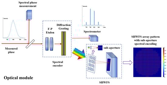
Figure 1.
Optical measurement module design diagram.
2.2. Parameter Analysis
In the optical module, an etalon and a diffraction grating were used for spectral encoding, and the microlens array of SHWFS was used for wavefront encoding. Precise optical component parameters are prerequisites for high spectral resolution and wavefront measurement accuracy. Therefore, the design parameters for these optical elements were calculated.
2.2.1. Fabry–Pérot Etalon
In our method, the Fabry–Pérot etalon is an important component for adjusting the spectral resolution and is employed to select discrete spectral components. The expanded spectral resolution depends on the free-spectral range :
For the 750–850 nm broadband pulse with a central wavelength of 800 nm, the free-spectral range corresponding to the 30 nm spectral resolution (four wavelengths) is 14 THz, and the 10 nm spectral resolution (ten wavelengths) requires a frequency of approximately 4.67 THz.
2.2.2. Diffractive Optical Element (Diffraction Grating)
The diffraction grating introduces a known dispersion into the measured pulse. This causes the spectral components to separate spatially on the detector after being focused by the microlens array. Based on the microlens imaging and the grating equation at normal incidence, we calculated the relationship in Equation (2): displacement on the SHWFS sub-aperture’s focal plane, which is caused by the grating dispersion of the spectral component relative to the central wavelength .
where f and d are the focal lengths of the sub-apertures and the grating constant (line/mm) respectively.
In the calculation, this displacement is manifested as an additional Zernike coefficient , which is expressed as:
where is the measurement zone radius of SHWFS. The derivation process is provided in Appendix A.
In addition, it is necessary to ensure that the edge spectra do not crosstalk with the adjacent sub-apertures. According to geometric optics, the relationship between the grating constant d and the parameters of the sub-apertures is:
where is the diameter of the sub-apertures, and is the edge wavelength. The derivation process is provided in Appendix A.
2.2.3. Structural Design of SHWFS
Traditional SHWFS employs a microlens array to encode the wavefront of the incident beam. The wavefront is then reconstructed using either a modal or zonal method based on the centroid displacement of the focal spot from each sub-aperture. In this study, we considered multispectral wavefront measurements and selected a neural network-based algorithm as the wavefront decoder. Consequently, when applying SHWFS to multispectral conditions, it is essential to consider both the size of the focal spot for individual spectral components and the number of distinct spectra that can be accommodated within a single microlens sub-aperture. Ideally, the focal spot of the SHWFS sub-aperture should be close to the diffraction limit. The number of pixels occupied in the detection plane is
where P is the pixel size of the detection plane.
According to Equations (2) and (5), our multi-spectral wavefront measurement approach requires a large aperture and short-focal-length SHWFS to accommodate focal spots with multi-wavelength components, thus improving the spectral resolution.
2.3. Neural Network Configuration
CNNs possess powerful image processing capabilities and have demonstrated high accuracy in large-scale image classification, defect detection, and weather forecasting. Similarly, a multi-spectral wavefront measurement task can be formulated as an end-to-end regression problem, thereby eliminating the need for spot centroid calculations. In a multi-wavelength SHWFS spot pattern, the spectra are incoherently combined, and the variation in each Zernike coefficient at each wavelength is encoded within the sub-aperture. By training on a large dataset, the neural network maps the focal spot pattern from the SHWFS to a reconstructed wavefront. Therefore, CNNs are highly effective decoders for end-to-end multispectral wavefront measurements. To avoid gradient vanishing while maintaining low loss function errors in the Zernike coefficient reconstruction, we implemented a Residual Shrinkage Network as a multi-spectral wavefront measurement model [38]. The training process is shown in Figure 2a; the CNN is trained using SHWFS spot patterns with shapes of (1000, 400) and its labels as inputs, with the corresponding Zernike coefficients as regression targets. The number of trainable parameters exceeds 30 million. During training, the network minimizes the loss function through iterative optimization. We selected the mean squared error (MSE) function as the loss function to evaluate the training effect. The model was trained with a batch size of 4 for a maximum of 200 epochs. An Adaptive Moment Estimation (Adam) optimizer with an initial learning rate of 0.0001 was used to update the network parameters, and early stopping ended the training when the validation loss was less than 5 × 10⁻⁵ over 15 consecutive epochs. The training terminates when either the maximum epoch count is reached or the validation loss meets the target threshold. The trained model output the predicted Zernike coefficients for each spectrum.
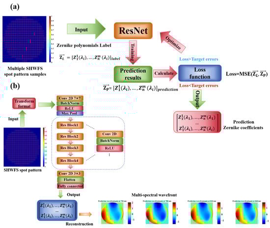
Figure 2.
Training process and neural network model structure. (a) Training process of CNN. (b) Measurement neural network structure.
Figure 2b shows the neural network structure, the model takes SHWFS spot patterns as input. A transfer function layer preprocesses the input, converting single-channel data into the three-channel format required by the ResNet model. The neural network first uses a 7 × 7 convolutional layer to extract sample feature, followed by a Batch Normalization (BN), a ReLU, and a max pooling layer that reduces the spatial dimensions while capturing primary features. Then, four residual blocks with convolutional layers, each structured as a “bottleneck” block utilizing a sequence of 1 × 1, 3 × 3, and 1 × 1 convolutional layer (each followed by BN and ReLU activation) to process the hierarchical feature. After feature extraction, a 3 × 3 convolutional layer condenses features, a flatten layer and a fully connected layer perform simultaneous regression of Zernike coefficients for multi-spectral. Zernike coefficients for multi-spectral are used for multi-spectral wavefront reconstruction and combined with spectral phase to characterize the spatio-temporal electric field.
2.4. Dataset Setup
A neural network was developed using a dataset of tens of thousands of SHWFS spot patterns and their corresponding Zernike coefficients for training and testing. A spectral resolution of 30 nm (wavelengths of 750, 780, 810, and 840 nm) was selected for the initial method validation, corresponding to an etalon free-spectral range of approximately 14 THz. According to the analysis and calculations presented in Section 2.2, the dataset employed an SHWFS configuration with 20 × 20 sub-apertures. Each microlens had a 4 mm focal length, with a sub-aperture spanning 50 pixels on the detector plane. Given a pixel resolution of 4 μm, this corresponded to a sub-aperture size of 200 × 200 μm. To enable direct accuracy comparison with the traditional centroid algorithm, Figure 3a,b illustrate the introduction of large dispersion (12 μm relative tip, corresponding to a 400 line/mm grating), ensuring complete spectral separation of the focal spots within each sub-aperture. Under these conditions, both the neural network model and the centroid algorithm measured the wavefront aberrations for each wavelength. Because spectral separation occurred exclusively along the x-axis, we symmetrically cropped 15 pixels from the top and bottom y-direction edges of each sub-aperture to eliminate unused data and reduce calculation time.
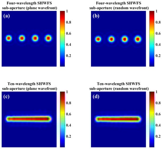
Figure 3.
SHWFS spot at sub-aperture (10, 10) as the example. (a,b) four separate spectral components with plane wavefront and a random wavefront. (c,d) Ten overlapping spectral components with plane wavefront and a random wavefront.
The neural network for the four-wavelength simulation was trained using 40,000 uniform randomly generated samples. Ten percent of the dataset was used for the validation set; that is, the training set contained 36,000 samples and the validation set contained 4000 samples. Additionally, a separate test dataset of 1000 new samples were generated to evaluate the model’s final generalization capability. The sample labels correspond to the Zernike coefficients that characterize the wavefront aberrations. Here, we selected orders 2nd–21st as the lower-order terms of primary interest in STC effects, excluding the piston term owing to its irrelevance to the wavefront distribution. Table 1 lists the values of the labeled Zernike coefficients. Given the limited wavefront variations between the spectral components under STC effects, we designated the 810 nm wavelength component as the reference (denoted ). For other wavelengths, each Zernike coefficient order was randomly generated within ±10% of the corresponding value. During training, these labels were normalized to the range to enhance the numerical stability of the model. Performance was quantified using the MSE between the predicted and true coefficients.

Table 1.
Zernike coefficients ranges of 2nd–21st orders.
As shown in Figure 3c,d, increasing the spectral resolution to 10 nm causes an incoherent focal spot overlap within each sub-aperture. The 10 target wavelengths spanned from 750 nm to 840 nm in 10 nm increments (750, 760, …, 840 nm), where the reference wavelength for the labeled Zernike coefficients was 800 nm and the label range was the same as that for the four-wavelength dataset. Under these conditions, the conventional centroid algorithm failed to resolve individual wavelengths, whereas the neural network model, trained on a large dataset could recognize unique focal spot patterns corresponding to each wavelength end-to-end. For ten-wavelength wavefront simulation, we selected the 4 μm relative tip displacement and expanded the training dataset to 50,000 samples, keeping all other parameters unchanged. In this work, we used a desktop workstation (Intel(R) Xeon(R) Silver 4210R CPU @ 2.40GHz, Kingston 128 GB, NVIDIA RTX2080 Ti) to generate data and train the models. The generation times of the four-wavelength and ten-wavelength datasets were 36 h and 111 h, respectively, and the training times were 17 h and 39 h respectively.
3. Results and Discussion
Once trained, the neural network model could simultaneously measure the multi-spectral wavefront from the corresponding SHWFS spot pattern. To evaluate the measurement performance of the neural network model, we used a test dataset of 1000 samples with label values distinct from the training data. The simulation accuracy and average processing time of the proposed approach were compared with those of a conventional modal method based on centroid displacement.
3.1. Simulation Results
The four-wavelength simulation results are presented in Table 2 and Figure 4; this measurement network has an average processing time of 21.38 ms per pattern. Initially, we calculated the root mean squared (RMS) accuracy of the input wavefront, predicted wavefront, and wavefront residuals for 1000 test dataset samples at four wavelengths, as presented in Figure 4a and Table 2. The RMS value of the reconstructed input wavefront was approximately 0.64 μm. The corresponding RMS wavefront residual errors for 750, 780, 810 and 840 nm wavelengths are 0.0086, 0.0079, 0.0090, and 0.0098 μm, respectively. Because the loss function of the neural network contains the Zernike coefficients for each wavelength component, there is a minor difference in the wavefront residuals for different wavelengths after the wavefront reconstruction statistics are performed. Furthermore, we also counted the peak-to-valley (PV) value of the wavefront residuals for the ultra-intense and ultra-short laser system. The PV values in Table 2 are the averages of the wavefront residual PV for the 1000 test dataset samples. The test dataset sample calculation results of the 2nd–21st-order Zernike coefficients and the wavefront reconstruction results at four wavelengths are presented in Figure 4b,c, which also show the high synchronization accuracy of the method. Based on previous studies, neural network measurement accuracy improves as the training dataset expands to sufficiently sample the Zernike coefficient space, whereas the prediction speed scales with computational resources.
Table 2.
Wavefront aberration of four wavelengths during simulation (1000 test dataset samples).
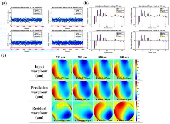
Figure 4.
Four-wavelength numerical simulation results. (a) RMS wavefront for 1000 test dataset samples at four-wavelength. (b) Simulation results of 2nd–21st-order Zernike coefficients at four wavelengths. (c) Reconstructed input wavefront, predicted wavefront and wavefront residuals at 750, 780, 810, and 840 nm of a test dataset sample.
3.2. Effect of Zernike Order on Reconstruction Accuracy
In Section 3.1, we presented the simulation performance of the NN model for a 4-wavelength wavefront defined by 2nd to 21st-order Zernike coefficients. In this section, we varied the Zernike order range of the samples and compared the simulation accuracy of the NN models.
Specifically, we selected samples with Zernike coefficients from 2nd–10th and 2nd–36th orders to compare the reconstruction accuracy. The sample metadata remained consistent with the previous section. As shown in Table 3, which compared the wavefront residuals of 1000 test samples under these three conditions, it was evident that with a fixed number of training samples, the RMS and PV values of the wavefront residuals decrease significantly as the maximum Zernike modes increased. This was attributed to the expansion of the parameter space, which reduced the sampling density of the training data.
Table 3.
Comparison of wavefront residuals across different Zernike modes (1000 test dataset samples).
3.3. Performance Comparison
Traditional SHWFS algorithms, such as modal and zonal approaches, utilize centroid displacements to calculate the wavefront slopes for reconstruction. In this study, we developed a modal-based SHWFS wavefront reconstruction algorithm, and compared its multi-wavelength wavefront reconstruction performance with that of our neural network method.
We initially employed a single-spectrum SHWFS spot pattern to verify the accuracy of our modal-based algorithm. The modal method based on centroid displacement showed highly reconstructed wavefront residuals with 0.0022 μm RMS accuracy in 100 samples of random 2nd–21st-order Zernike coefficients (the range of Zernike coefficients is the same as in Section 3.1). For the higher-order Zernike coefficients (36th, 78th, and 120th), the RMS residuals of the reconstructed wavefront averaged over 100 samples were 0.0049 µm, 0.056 µm, and 0.15 µm, respectively.
As illustrated in Figure 5a–c, we divided each SHWFS sub-aperture into four rectangular regions to isolate the different spectral components for centroid calculation. However, the accuracy of synchronously measuring the four-wavelength wavefront aberrations using the modal method decreased significantly. Figure 6 compares the predicted wavefront and wavefront residuals of the same SHWFS spot pattern using the neural network-based method and the centroid displacement modal method at the four wavelengths. The reconstructed RMS wavefront residual error of the modal method achieved only approximately 0.090 μm, its accuracy is significantly less than that of the neural network method. As illustrated in Figure 5c, owing to the insufficient distance between the focal spots of different wavelengths on the SHWFS sub-aperture, wavefront aberrations lead to crosstalk between adjacent focal spots, ultimately affecting the calculation of the centroid displacement.
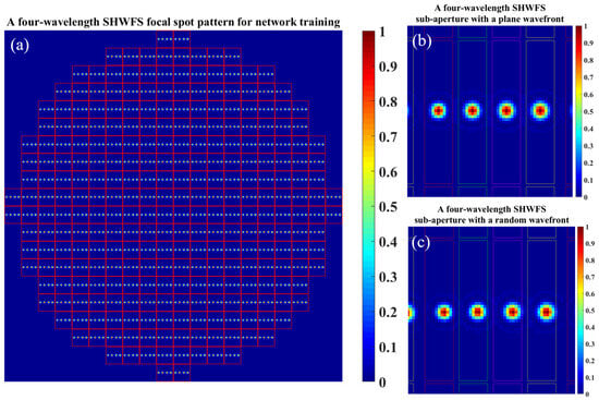
Figure 5.
The four regions divided on SHWFS spot pattern and a sub-aperture. (a) SHWFS spot pattern samples for training and testing. (b) SHWFS sub-aperture with plane wavefront. (c) SHWFS sub-aperture with random wavefront.
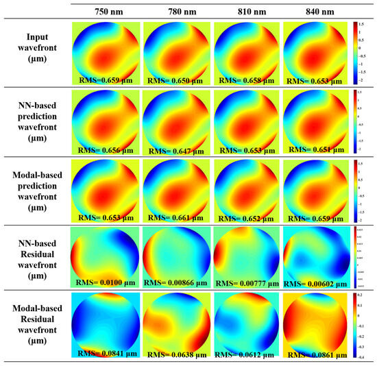
Figure 6.
Wavefront reconstruction results of neural network-based and centroid displacement-based modal methods.
3.4. Multi-Spectral Research
A high spectral resolution allows for a more accurate reconstruction of spatio-temporal electric fields. In this section, we extended the approach to simultaneous processing at ten wavelengths, which corresponded to a spectral resolution of 10 nm. Note that the spectral resolution of our method can be further enhanced by optimizing the structural parameters of the individual SHWFS microlenses, although this requires increased sample generation and training time. The ten-wavelength SHWFS spot pattern samples are shown in Figure 7, where the focal spots of different wavelengths spatially overlap on the SHWFS sub-aperture, resulting in the failure of the conventional centroid algorithm. Nevertheless, the wavefront aberrations at different wavelengths exert distinct effects on the individual SHWFS sub-apertures. The neural network model captures and differentiates these features and continuously converges to the target threshold during training while maintaining high simulation accuracy. The wavefront calculation results for the ten-wavelength are shown in Figure 8a–j, where the average wavefront reconstruction time remains at 21.82 ms per pattern. The wavefront residuals of ten wavelengths in the test dataset are listed in Table 4. Compared to four wavelengths, the simulation accuracy of the network decreases due to the increased number of regressed parameters, but still maintains a high synchronization accuracy of about 0.016 μm.
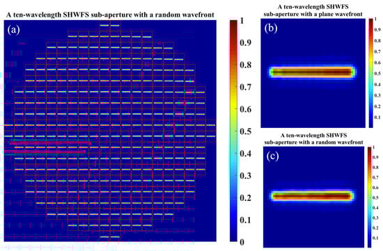
Figure 7.
SHWFS spot pattern and a sub-aperture with ten wavelengths. (a) Ten-wavelength SHWFS spot pattern samples for training and testing. (b) SHWFS sub-aperture with plane wavefront. (c) SHWFS sub-aperture with random wavefront.
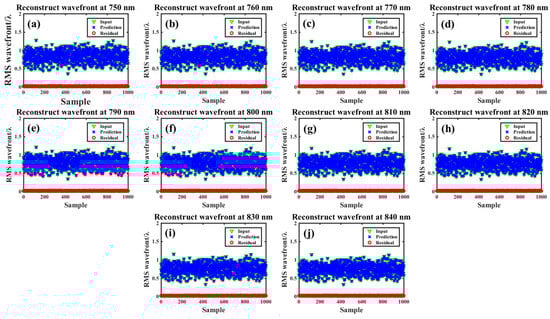
Figure 8.
Ten-wavelength wavefront reconstruction results for 1000 test dataset samples. (a–j) Results at wavelengths from 750 nm to 840 nm in 10 nm increments.
Table 4.
Wavefront aberration of ten wavelengths during simulation (1000 test dataset samples).
3.5. Discussion
In this section, we present the numerical simulation results of a neural network model for synchronous four-wavelength and ten-wavelength wavefront aberration measurements on a single SHWFS. The superiority of the deep learning method over the traditional SHWFS centroid algorithm is also verified. Theoretically, enhancing the spectral resolution requires the use of a Fabry–Pérot etalon with a narrower free spectral range. Correspondingly, a grating with a smaller constant provides a larger dispersion angle for each spectrum, thereby increasing the separation in the SHWFS spot pattern. In turn, a microlens array with larger sub-apertures is required to accommodate more dispersed spectral components. For the image sensor, smaller pixel units (commercially available down to 2 μm) can resolve finer focal spot details, thereby improving wavefront reconstruction resolution. However, these improvements require a more extensive dataset for neural network training. Furthermore, increasing the sub-aperture size or reducing the pixel size substantially increases the computational data load. Therefore, a balance must be struck between the data volume and resolution. In addition, this method can be adapted to other spectral bands. Indeed, this adaptability requires careful consideration of the optical parameters, as any change in wavelength range alters both the focal spot size of the microlens array and the response curve of grating. These changes must be accounted for by optimizing the optical component parameters for the target spectrum. In the STC effect, low-frequency PFT and PFC are the primary concerns. This study mainly used the Zernike coefficients from the 2nd to 21st order to reconstruct the multispectral wavefront, which meets the requirements of STC effect detection. Higher-order wavefront reconstructions demand substantially increased training samples and computational resources, causing the reconstruction accuracy to decrease as the Zernike orders increase.
In future work, we will focus on validating the method in ultra-intense and ultra-short laser systems, which requires customizing etalons with an appropriate free spectral range and SHWFS with special microlens sizes. In terms of software, the expanded training dataset and reduced loss function threshold during training have the potential to further improve measurement accuracy. Furthermore, using some new convolutional neural network architectures developed in recent years, such as RepViT or a hybrid CNN with U-net/Transformer, also has the potential to improve measurement performance and computational efficiency.
4. Conclusions
In conclusion, a neural network-based multi-spectral and single-shot wavefront detection technique was presented. This approach employs a Fabry–Pérot etalon to select the measured spectral components, followed by the introduction of a frequency-dependent linear dispersion using a diffractive optical element. Thus, the individual spectral components are separated on the focal plane of each SHWFS sub-aperture. Utilizing the target spectra, introduced dispersion, and SHWFS design parameters, the SHWFS spot pattern samples were generated to train a ResNet-based measurement neural network. In the numerical simulations, we initially demonstrated the simultaneous simulation of 4-wavelength, 21st-order Zernike coefficients. The measurement network model achieves an average calculation time of 21.38 ms and an RMS wavefront residual error of 0.010 μm. This processing performance has significant advantages over traditional SHWFS centroid algorithms. Meanwhile, numerical simulations demonstrated that the reconstruction accuracy of this method decreases for higher-order Zernike modes. When the spectral resolution is increased to 10 nm, the centroid algorithms fail due to overlapping spots on the SHWFS sub-apertures; the neural network maintains high accuracy, achieving an RMS wavefront residuals error of 0.016 μm. In addition, the theoretical spectral resolution can be increased by optimizing the microlens array parameters. This technique expands the application of SHWFS in the frequency-domain, which is especially suitable for the measurement of spatio-temporal electric field characterization in low-repetition-rate or even single-shot ultra-intense ultrashort laser systems. In the future, we will explore the practical applications of this technique.
Author Contributions
Conceptualization, X.L. (Xunzheng Li) and L.Y.; methodology, X.L. (Xunzheng Li); software, X.L. (Xunzheng Li); validation, X.L. (Xunzheng Li) and A.W.; formal analysis, X.L. (Xunzheng Li); resources, L.Y. and X.L. (Xiaoyan Liang); writing—original draft preparation, X.L. (Xunzheng Li); writing—review and editing, M.F., L.Y. and X.L. (Xiaoyan Liang), all authors. All authors have read and agreed to the published version of the manuscript.
Funding
This work was supported by various the funding sources: National Key Research and Development Program of China under Grant No. 2023YFA1608502, Youth Innovation Promotion Association of the Chinese Academy of Sciences under Grant No. 2019247, and Strategic Priority Research Program of the Chinese Academy of Sciences under Grant No. XDB0890100.
Data Availability Statement
The data that support the findings of this study are available from the corresponding author upon reasonable request.
Conflicts of Interest
The authors declare no conflicts of interest.
Abbreviations
The following abbreviations are used in this manuscript:
| SHWFS | Shack–Hartmann Wavefront Sensor |
| RMS | Root mean squared |
| AO | Adaptive optics |
| STC | Spatio-temporal coupling |
| PFT | Pulse-front tilt |
| PFC | Pulse-front curvature |
| SID4 | Four-wave lateral shearing interferometer |
| CNN | Convolutional neural network |
| DL | Deep learning |
| ResNet | Residual Shrinkage Network |
| NN | Neural networks |
| MSE | Mean squared error |
| BN | Batch Normalization |
| PV | Peak-to-valley |
Appendix A
The derivation of Equation (3):
For the tip (x-tip, y-tilt) term, the wavefront W can be written as:
where is the tip value.
The Zernike polynomial of in polar and Cartesian coordinates system is defined as:
where and are the normalized radial and angular coordinates in the polar coordinate system, x is the position coordinate in the Cartesian coordinate system, and R denotes the beam radius. For a tilted wavefront, the relationship between the tilt value and the deflection angle () is:
According to the grating equation (d is the grating constant):
Under normal incidence , the +1st-order diffraction angle of is
Therefore, the relationship of Equation (A6) can be obtained:
where is the measurement zone radius of SHWFS.
The derivation of Equation (4):
The edge spectra do not crosstalk with adjacent sub-lens, according to geometric optics:
where is the radius of the edge spectral focal spot.
By combining Equations (A4) and (A8), we can derive Equation (A9):
References
- Lureau, F.; Matras, G.; Chalus, O.; Derycke, C.; Morbieu, T.; Radier, C.; Casagrande, O.; Laux, S.; Ricaud, S.; Rey, G.; et al. High-energy hybrid femtosecond laser system demonstrating 2 × 10 PW capability. High Power Laser Sci. 2020, 8, e43. [Google Scholar] [CrossRef]
- Guo, Z.; Yu, L.H.; Wang, J.Y.; Wang, C.; Liu, Y.Q.; Gan, Z.B.; Li, W.Q.; Leng, Y.X.; Liang, X.Y.; Li, R.X. Improvement of the focusing ability by double deformable mirrors for 10-PW-level Ti: Sapphire chirped pulse amplification laser system. Opt. Express 2018, 26, 26776–26786. [Google Scholar] [CrossRef] [PubMed]
- Samarkin, V.V.; Alexandrov, A.G.; Galaktionov, I.; Kudryashov, A.; Nikitin, A.N.; Rukosuev, A.L.; Toporovsky, V.V.; Sheldakova, Y. Large-aperture adaptive optical system for correcting wavefront distortions of a petawatt Ti: Sapphire laser beam. Quantum Electron. 2022, 52, 187–194. [Google Scholar] [CrossRef]
- Dai, G.-M. Modified Hartmann-Shack wavefront sensing and iterative wavefront reconstruction. In Proceedings of the Adaptive Optics in Astronomy, Kona, HI, USA, 17–18 March 1994; pp. 562–573. [Google Scholar]
- Fried, D.L. Least-square fitting a wave-front distortion estimate to an array of phase-difference measurements. J. Opt. Soc. Am. 1977, 67, 370–375. [Google Scholar] [CrossRef]
- Roberts, L.C.; Neyman, C.R. Characterization of the AEOS adaptive optics system. Publ. Astron. Soc. Pac. 2002, 114, 1260–1266. [Google Scholar] [CrossRef]
- Liang, J.Z.; Grimm, B.; Goelz, S.; Bille, J.F. Objective Measurement of Wave Aberrations of the Human Eye with the Use of a Hartmann-Shack Wave-Front Sensor. J. Opt. Soc. Am. A-Opt. Image Sci. Vis. 1994, 11, 1949–1957. [Google Scholar] [CrossRef]
- Pastrana, E. Adaptive optics for biological imaging. Nat. Methods 2011, 8, 45. [Google Scholar] [CrossRef]
- Dorn, A.; Zappe, H.; Ataman, Ç. Conjugate adaptive optics extension for commercial microscopes. Adv. Photonics Nexus 2024, 3, 056018. [Google Scholar] [CrossRef]
- Ohland, J.B.; Lebas, N.; Deo, V.; Guyon, O.; Mathieu, F.; Audebert, P.; Papadopoulos, D. Apollon Real-Time Adaptive Optics: Astronomy-inspired wavefront stabilization in ultraintense lasers. High Power Laser Sci. 2025, 13, e29. [Google Scholar] [CrossRef]
- Zhang, Y.W.; Dinh, M.; Wang, Z.Y.; Zhang, T.H.; Chen, T.H.; Hsu, C.W. Adaptive optical multispectral matrix approach for label-free high-resolution imaging through complex scattering media. Adv. Photonics 2025, 7, 046008. [Google Scholar] [CrossRef]
- Jolly, S.W.; Gobert, O.; Quéré, F. Spatio-temporal characterization of ultrashort laser beams: A tutorial. J. Opt. 2020, 22, 103501. [Google Scholar] [CrossRef]
- Li, Z.; Tsubakimoto, K.; Yoshida, H.; Nakata, Y.; Miyanaga, N. Degradation of femtosecond petawatt laser beams: Spatio-temporal/spectral coupling induced by wavefront errors of compression gratings. Appl. Phys. Express 2017, 10, 102702. [Google Scholar] [CrossRef]
- Li, Z.Y.; Miyanaga, N. Simulating ultra-intense femtosecond lasers in the 3-dimensional space-time domain. Opt. Express 2018, 26, 8453–8469. [Google Scholar] [CrossRef] [PubMed]
- Li, Z.Y.; Miyanaga, N.; Kawanaka, J. Single-shot real-time detection technique for pulse-front tilt and curvature of femtosecond pulsed beams with multiple-slit spatiotemporal interferometry. Opt. Lett. 2018, 43, 3156–3159. [Google Scholar] [CrossRef] [PubMed]
- Bor, Z. Distortion of Femtosecond Laser-Pulses in Lenses. Opt. Lett. 1989, 14, 119–121. [Google Scholar] [CrossRef]
- Jeandet, A.; Borot, A.; Nakamura, K.; Jolly, S.W.; Gonsalves, A.J.; Tóth, C.; Mao, H.-S.; Leemans, W.P.; Quéré, F. Spatio-temporal structure of a petawatt femtosecond laser beam. J. Phys. Photonics 2019, 1, 035001. [Google Scholar] [CrossRef]
- Long, T.Y.; Wei, L.; Xu, H.T.; Xiao, W. Influence of spatiotemporal coupling distortion on evaluation of pulse-duration-charactrization and focused intensity of ultra-fast and ultra-intensity laser. Acta Phys. Sin. 2022, 71, 174204. [Google Scholar] [CrossRef]
- Li, W.Q.; Gan, Z.B.; Yu, L.H.; Wang, C.; Liu, Y.Q.; Guo, Z.; Xu, L.; Xu, M.; Hang, Y.; Xu, Y.; et al. 339 J high-energy Ti:sapphire chirped-pulse amplifier for 10 PW laser facility. Opt. Lett. 2018, 43, 5681–5684. [Google Scholar] [CrossRef]
- Radier, C.; Chalus, O.; Charbonneau, M.; Thambirajah, S.; Deschamps, G.; David, S.; Barbe, J.; Etter, E.; Matras, G.; Ricaud, S.; et al. 10 PW peak power femtosecond laser pulses at ELI-NP. High Power Laser Sci. 2022, 10, e21. [Google Scholar] [CrossRef]
- Chanteloup, J.C.; Cohen, M. Compact, high resolution, four wave lateral shearing interferometer. Opt. Fabr. Test. Metrol. 2004, 5252, 282–292. [Google Scholar]
- Shack, R.V.; Platt, B.C. Production and Use of a Lenticular Hartmann Screen. J. Opt. Soc. Am. 1971, 656. [Google Scholar]
- Xu, Y.M.; Jin, C.Z.; Pan, L.Z.; He, Y.; Yao, Y.H.; Qi, D.L.; Liu, C.; Shi, J.H.; Sun, Z.R.; Zhang, S.; et al. Single-shot spatial-temporal-spectral complex amplitude imaging via wavelength-time multiplexing. Adv. Photonics 2025, 7, 026004. [Google Scholar] [CrossRef]
- Bowlan, P.; Gabolde, P.; Trebino, R. Directly measuring the spatio-temporal electric field of focusing ultrashort pulses. Opt. Express 2007, 15, 10219–10230. [Google Scholar] [CrossRef]
- Cousin, S.L.; Bueno, J.M.; Forget, N.; Austin, D.R.; Biegert, J. Three-dimensional spatiotemporal pulse characterization with an acousto-optic pulse shaper and a Hartmann-Shack wavefront sensor. Opt. Lett. 2012, 37, 3291–3293. [Google Scholar] [CrossRef] [PubMed]
- Kim, Y.G.; Kim, J.I.; Yoon, J.W.; Sung, J.H.; Lee, S.K.; Nam, C.H. Single-shot spatiotemporal characterization of a multi-PW laser using a multispectral wavefront sensing method. Opt. Express 2021, 29, 19506–19514. [Google Scholar] [CrossRef] [PubMed]
- Ren, Z.B.; Xu, Z.M.; Lam, E.Y. End-to-end deep learning framework for digital holographic reconstruction. Adv. Photonics 2019, 1, 016004. [Google Scholar] [CrossRef]
- Wang, H.D.; Rivenson, Y.; Jin, Y.Y.; Wei, Z.S.; Gao, R.; Günaydin, H.; Bentolila, L.A.; Kural, C.; Ozcan, A. Deep learning enables cross-modality super-resolution in fluorescence microscopy. Nat. Methods 2019, 16, 103–110. [Google Scholar] [CrossRef] [PubMed]
- Barbastathis, G.; Ozcan, A.; Situ, G. On the use of deep learning for computational imaging. Optica 2019, 6, 921–943. [Google Scholar] [CrossRef]
- Hu, L.; Hu, S.; Gong, W.; Si, K. Learning-based Shack-Hartmann wavefront sensor for high-order aberration detection. Opt. Express 2019, 27, 33504–33517. [Google Scholar] [CrossRef]
- Hu, L.; Hu, S.; Gong, W.; Si, K. Deep learning assisted Shack-Hartmann wavefront sensor for direct wavefront detection. Opt. Lett. 2020, 45, 3741–3744. [Google Scholar] [CrossRef]
- He, Y.L.; Liu, Z.W.; Ning, Y.; Li, J.; Xu, X.J.; Jiang, Z.F. Deep learning wavefront sensing method for Shack-Hartmann sensors with sparse sub-apertures. Opt. Express 2021, 29, 17669–17682. [Google Scholar] [CrossRef]
- Zhao, M.M.; Zhao, W.; Wang, S.; Yang, P.; Yang, K.J.; Lin, H.Q.; Kong, L.X. Centroid-Predicted Deep Neural Network in Shack-Hartmann Sensors. IEEE Photonics J. 2022, 14, 6804810. [Google Scholar] [CrossRef]
- Ziemann, M.R.; Rathbun, I.A.; Metzler, C.A. A learning-based approach to event-based shack-hartmann wavefront sensing. In Proceedings of the Unconventional Imaging, Sensing, and Adaptive Optics 2024, San Diego, CA, USA, 18–23 August 2024; pp. 199–207. [Google Scholar]
- Qiao, C.; Chen, H.Y.; Wang, R.; Jiang, T.; Wang, Y.W.; Li, D. Deep learning-based optical aberration estimation enables offline digital adaptive optics and super-resolution imaging. Photonics Res. 2024, 12, 474–484. [Google Scholar] [CrossRef]
- Tang, H.C.; Men, T.; Liu, X.L.; Hu, Y.D.; Su, J.Q.; Zuo, Y.L.; Li, P.; Liang, J.Y.; Downer, M.C.; Li, Z.Y. Single-shot compressed optical field topography. Light-Sci. Appl. 2022, 11, 244. [Google Scholar] [CrossRef]
- Wirth-Singh, A.; Xiang, J.; Choi, M.; Fröch, J.E.; Huang, L.; Colburn, S.; Shlizerman, E.; Majumdar, A. Compressed meta-optical encoder for image classification. Adv. Photonics Nexus 2025, 4, 026009. [Google Scholar] [CrossRef]
- He, K.M.; Zhang, X.Y.; Ren, S.Q.; Sun, J. Deep Residual Learning for Image Recognition. In Proceedings of the 2016 IEEE Conference on Computer Vision and Pattern Recognition (CVPR), Las Vegas, NV, USA, 27–30 June 2016; pp. 770–778. [Google Scholar]
Disclaimer/Publisher’s Note: The statements, opinions and data contained in all publications are solely those of the individual author(s) and contributor(s) and not of MDPI and/or the editor(s). MDPI and/or the editor(s) disclaim responsibility for any injury to people or property resulting from any ideas, methods, instructions or products referred to in the content. |
© 2025 by the authors. Licensee MDPI, Basel, Switzerland. This article is an open access article distributed under the terms and conditions of the Creative Commons Attribution (CC BY) license (https://creativecommons.org/licenses/by/4.0/).