Indoor Visible Light Positioning Based on Channel Estimation and Cramér–Rao Low Bound Analysis with Random Receiving Orientation of User Equipment

Abstract

The accuracy of line-of-sight (LOS)-based indoor visible light positioning (VLP) depends directly on the accuracy of the received LOS power. In an actual indoor visible light communication (VLC) system, the total received power contains the LOS power and diffuse power, and the proportion of diffuse component varies significantly with the receiving orientation of the user equipment (UE). In the trilateration positioning process, this is bound to bring a very high level of inaccuracy for at least one or two of them when determining the distance between the positioned LED and UE. To solve this problem, we employed channel estimation and Parseval’s theorem to remove the diffuse component from the total received power. The simulation results show that the higher the channel estimation accuracy, the smaller the discrepancy between the estimated and actual LOS power, and the greater the localization accuracy. At the same channel estimation accuracy, the comparison results demonstrate that the localization performance of the proposed method is higher than LLS-1, in which the total received power is directly adopted to estimate the distance. The localization performance of LLS-2 deteriorates significantly compared to the proposed method. This result indicates that the receiving orientation cannot be neglected during the distance estimation process even though the estimated accuracy of LOS power is high. Deriving the Cramér–Rao low bound (CRLB) for LOS-based indoor VLP with receiving orientation, we compared the localization performance for the proposed method with LLS-1, LLS-2, and the CRLB at various signal-to-noise ratios (SNRs). The results show that the localization error of all the received positions in the room can reach the CRLB at approximately 25 dB. However, localization errors based on LLS-1 and LLS-2 cannot achieve the theoretical CRLB even at a high SNR.

1. Introduction

To meet the growing demand for location-aware services, extensive research on wireless positioning technologies has been performed over the past decade [1]. Typically, a global positioning system (GPS) is used to provide location-aware services for the outdoor environment, yet it can hardly be used for applications such as tracking people and goods in smart factories, positioning and navigating automated guided vehicles, or underground parking lot vehicle guidance in various indoor application scenarios, where signals suffer from severe attenuation when passing through solid walls [2]. As a result, several alternatives, such as radio frequency identification (RFID) [3], Wi-Fi [4], ultra-wideband [5], and ZigBee [6], have emerged. However, these alternatives have limitations, owing to their low accuracy, electromagnetic interference, low security, and crowded spectrum resources. Visible light positioning (VLP) solutions that utilize visible light communication (VLC) systems for indoor positioning have attracted significant attention because of their unique advantages, such as wide license-free bandwidth, low electromagnetic interference, low costs, and high security, which are expected to result in improved positioning accuracy [7,8].

Researchers have proposed a variety of non-imaging receiving positioning methods, including angle of arrival (AOA) [9], time of arrival (TOA) [10], time difference of arrival (TDOA) [11], and received signal strength (RSS) [12]. The RSS-based algorithm does not require precise synchronization between devices nor complex receivers, and it has attracted increasing attention.

The main branches of RSS-based algorithms include trilateration and fingerprinting positioning algorithms. Fingerprinting has been proven to have higher accuracy when combined with machine learning algorithms [13,14,15]. However, it is generally laborious and time-consuming to collect specific parameters through site surveys when constructing a sample database in the offline stage. The trilateration positioning algorithm, which uses a single photodiode (PD) and three LEDs distributed on the ceiling, exhibits lower implementation and time complexity and strong adaptability to a variety of indoor environments; hence, it has become a widely studied method [16,17].

In practice, the optical signal is delivered to the receiver via line-of-sight (LOS) and diffuse paths. Thus, the total received power consists of the LOS and diffuse components. This diffuse component is the superposition of all non-line-of-sight (NLOS) components due to one or more reflections on the wall surfaces [18]. Regarding the trilateration positioning algorithms, the channel gain model used to estimate the distances between the LED transmitters and receiver only considers the LOS power attenuation. That is, the more accurate the LOS component power extracted from the total received power, the more accurate is the estimation of the distance [19]. The majority of studies on the trilateration positioning algorithms assume that both LED transmitters and receivers are oriented perpendicular to the room ceiling. The diffuse component was considered to be less than 10%, and the total received power was primarily the LOS component [19]. In these studies, the LOS power attenuation was replaced by the total received power to estimate the distance between the LED transmitter and receiver, while the diffuse component was ignored completely [20,21,22]. However, such assumptions are not accurate for users who carry mobile devices such as smartphones. They tend to hold their devices in a way that feels the most comfortable, whether moving or stationary [23,24]. In these real-life scenarios, the assumption of perfect alignment between the receiving orientation and LED transmitter orientation is not valid. Nevertheless, certain studies have been conducted on this issue. Considering only the LOS link, an enhanced trilateration positioning method has been proposed to improve the localization accuracy, in which the maximum location error increases twice under the effect of receiving orientation when the polar angle is equal to $\theta =\pi /6$ [25]. In [17,26], the trilateration positioning that uses an angle diversity transmitter and an RSS-assisted perspective-three-point algorithm provided decimeter-level accuracy by only considering the LOS link. In fact, a change in the receiving orientation led to a change in the angle of incidence, which directly influenced both the LOS and diffuse components. However, the positioning accuracy is significantly affected if the the LOS component cannot be accurately estimated.

Considering the actual receiving orientation of UE, this work attains highly accurate positioning under NLOS multipath effects through channel estimation and Parseval’s theorem. The proposed scheme avoids complex mathematical modeling of NLOS transmission, which depends on room dimensions, walls, reflectivity, UE location and orientation, and LED location. It utilizes the existing VLC downlink to infer the position of UE without requiring extra hardware facilities and complex algorithms and is an efficient localization method suitable for practical indoor scenarios.

The main contributions of this work are as follows:

• Analysis of influence for random receiving orientation on the proportion of the diffuse component to the total received power, in which the influencing factors consist of the yaw, pitch, and roll angles;
• Proposal of a novel trilateration positioning algorithm based on channel estimation and Parseval’s theorem, which can accurately estimate the proportion of diffuse power to the total received power;
• Derivation of the CRLB for the LOS-based indoor VLP under the effect of the receiving orientation;
• Evaluation of the proposed positioning scheme in an actual indoor positioning scene by extensive computer simulation comparisons with the CRLB for different SNRs.

The remainder of this paper is arranged as follows: The channel model is presented in Section 2. The proposed VLP scheme is presented in Section 3. Section 4 presents the Cramér–Rao low bound for the positioning estimation error. The numerical results and discussion are presented in Section 5. Finally, Section 6 concludes the paper.

2. Channel Model for Wireless Optical Communication

The VLC-based localization geometric model for a typical indoor scene where the length, width, and height are 5 m, 5 m, and 3 m, respectively, is shown in Figure 1. There are four LEDs mounted on the ceiling as transmitters, and the user is holding a mobile phone equipped with a PD receiver, represented by user equipment (UE), whose location is to be inferred. The technical parameters of the geometric model, LED transmitters, and PD receiver, are provided in Table 1.

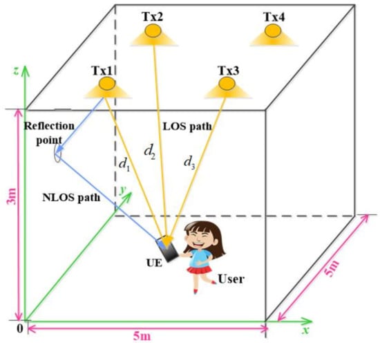
Figure 1. Typical indoor VLC-based localization geometric model.

Table 1. Geometric model technical parameters.

Room Parameters	Room Dimensions	$5\mathrm{m}\times 5\mathrm{m}\times 3\mathrm{m}$
	Reflectivity of the Walls	0.6
Transmitter Parameters	Maximum transmitted optical power per LED	1.5 W
	Minimum transmitted optical power per LED	0.5 W
	Number of LEDs	4
	Half power semi-angle (${\mathrm{\Phi }}_{\frac{1}{2}}$)	$60°$
	Field of view of the LEDs ($\mathrm{\Phi }$)	$90°$
	Bandwidth of LED	50 MHz
	Position of LED1	Tx1 (−1.5, −1.5, 3)
	Position of LED2	Tx2 (−1.5, 1.5, 3)
	Position of LED3	Tx3 (1.5, −1.5, 3)
	Position of LED4	Tx4 (1.5, 1.5, 3)
Receiver Parameters	Height of UE $\left(h\right)$	$0.85\mathrm{m}$
	Effective detecting area ($A_{\mathrm{PD}}$)	$1{\mathrm{cm}}^2$
	Gain of the optical filter ($T_{\mathrm{s}}$)	1
	Refractive index (n)	1
	Field of view of the PDs ($\mathrm{\Psi }$)	$90°$
	Responsivity ($\gamma$)	$0.6$ A/W
	System bandwidth (B)	10 MHz
	Noise power spectral density ($N_0$)	${10}^{-21}\mathrm{W}/\mathrm{Hz}$

The optical channel model, which consists of the LOS link and diffuse link that includes one or more reflections from wall surface, is shown in Figure 2. In the following, the LOS channel, diffuse channel, and overall optical channels are discussed.

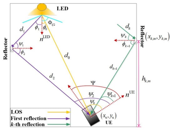
Figure 2. The LOS and diffuse optical channel models for one LED.

2.1. The LOS Channel

The time-domain impulse response of the LOS channel is given by:

$$h_{\mathrm{LOS}}\left(t\right)=g_{\mathrm{L}}\delta (t-{\tau }_{\mathrm{Rx},\mathrm{Tx}}),$$

(1)

where $g_{\mathrm{L}}$ is the generalized Lambertian radiator with an attenuation factor between the transmitter and UE; its expression is given by Equation (4) [17]. ${\tau }_{\mathrm{Rx},\mathrm{Tx}}=d_0/c$ is the signal propagation delay between the transmitter and UE, c is the speed of light, and $d_0$ is the distance between the transmitter and UE.

$$g_{\mathrm{L}}=\left\{\begin{array}{c}\frac{\left(m+1\right)A_{\mathrm{PD}}}{2\pi d_0^2}{cos}^m\left({\varphi }_0\right)cos\left({\psi }_0\right)T_{\mathrm{s}}\left({\psi }_0\right)G\left({\psi }_0\right)0<{\psi }_0<\mathrm{\Psi },\hfill \\ 0\mathrm{otherwise},\hfill \end{array}\right.$$

(2)

where $m=-\frac{ln2}{ln\left(cos{\mathrm{\Phi }}_{1/2}\right)}$ is the order of Lambertian emission; ${\mathrm{\Phi }}_{1/2}$ is the half-power semi-angle; $A_{\mathrm{PD}}$ is the effective detector area of the PD; ${\varphi }_0$ and ${\psi }_0$ are, respectively, the irradiance and incidence angles from the LED to the PD; $T\left({\psi }_0\right)$ and $G\left({\psi }_0\right)$ are the optical filter gain and concentrator gain of the PD receiver, respectively; and $\mathrm{\Psi }$ represents the field of view (FOV) of the receiver.

When the normal vector of the receiver is no longer vertically upward, it is no longer valid to let the incident angle ${\psi }_0$ simply equal ${cos}^{-1}\left(\frac{h}{d_0}\right)$ in Equation (2). In this general case, the incidence angle is determined by the positions of the transmitter and UE, as well as the UE orientation. This is then given by [25]:

$${\psi }_0={cos}^{-1}\left[\frac{\left(x-x_{\mathrm{u}}\right)sin\theta sin\omega +\left(y-y_{\mathrm{u}}\right)sin\theta sin\omega +hcos\theta }{d_0}\right],$$

(3)

where $\left(x,y\right)$ and $\left(x_{\mathrm{u}},y_{\mathrm{u}}\right)$ are the coordinates of the transmitter and UE, respectively. Polar angle $\theta$ and azimuth angle $\omega$ are used to describe the random receiver orientation, as shown in Figure 3. The former denotes the angle between the receiver normal vector and z-axis, whereas the azimuth angle is between the receiver normal vector and x-axis in the xy-plane. The orientation of the receiver can be extracted from the three fundamental rotation angles obtained from the built-in sensor of the smartphone. These angles denote rotations about the z-axis, x-axis, and y-axis, as illustrated in Figure 3 of [24], which are represented by $\alpha$, $\beta$, and $\gamma$, respectively. According to Euler’s rotation theorem, the polar angle and azimuth angle can be represented by the fundamental rotation angles as [25]:

$$\theta =arccos\left(cos\beta cos\gamma \right),$$

(4)

$$\omega =arctan\frac{sin\alpha sin\gamma -cos\alpha cos\gamma sin\beta }{cos\gamma sin\alpha sin\beta +cos\alpha sin\gamma }.$$

(5)

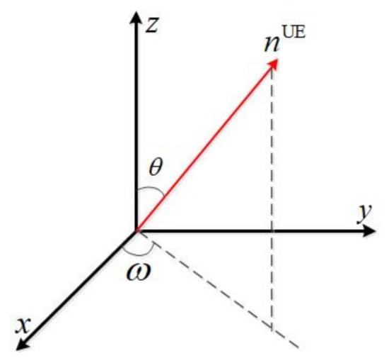
Figure 3. Schematic diagram of the user’s random receiving orientation.

It is evident that the polar angle $\theta$ depends on the rotations of the x- and y-axes, which are related to the user’s hand movement. The azimuth angle $\omega$ is determined by all fundamental rotation angles.

2.2. The Diffuse Channel

The diffuse link is the sum of the contributions from all non-LOS links that are due to one or more reflections between the wall surfaces. A discrete reflector model was obtained by dividing the walls into small surface elements, denoted by $A_{\mathrm{ref}}$. Each surface element itself acts as a radiator by reflecting the impinging light, thereby reducing the optical power through the reflectivity factor ${\rho }_k$, which is related to the wall materials. The impulse response $h_{\mathrm{DIFF}}\left(t\right)$ for the diffuse channel is approximated by the sum of the contributions from reflections up to a given order $N_{\mathrm{nef}}$ [18]:

$$h_{\mathrm{DIFF}}\left(t\right)\approx \sum _{k=1}^{N_{\mathrm{ref}}}{h}_{\mathrm{DIFF}}^{\left(k\right)}\left(t\right).$$

(6)

The response $h_{\mathrm{DIFF}}^{\left(k\right)}\left(t\right)$ after k-reflection to the LED source is given by [18]:

$$h_{\mathrm{DIFF}}^{\left(k\right)}\left(t\right)=\left\{\begin{array}{c}{\int }_S(L_1·L_2·\dots ·L_{k+1})·{\rho }_1·{\rho }_2·\dots ·{\rho }_k·\delta (t-\frac{d_1+d2+\dots +d_{k+1}}{c})d{A}_{\mathrm{ref}}0<{\psi }_0<\mathrm{\Psi },\hfill \\ 0\mathrm{otherwise},\hfill \end{array}\right.$$

(7)

The path-loss terms for each path in Equation (7) are given as [18]:

$$\begin{array}{cc}\hfill L_1& =\frac{A_{\mathrm{ref}}(m+1)}{2\pi d_1^2}{\mathit{cos}}^m\left({\varphi }_1\right)\mathit{cos}\left({\psi }_1\right),\hfill \\ \hfill L_2& =\frac{A_{\mathrm{ref}}}{\pi d_2^2}\mathit{cos}\left({\varphi }_2\right)\mathit{cos}\left({\psi }_2\right),\dots ,\hfill \\ \hfill L_{k+1}& =\frac{A_{\mathrm{PD}}}{\pi d_{k+1}^2}\mathit{cos}\left({\varphi }_{k+1}\right)\mathit{cos}\left({\psi }_{k+1}\right).\hfill \end{array}$$

The incident angle ${\psi }_{k+1}$ in the path-loss term $L_{k+1}$ cannot be simply replaced by ${\cos }^{-1}\left(\frac{h_{k+1}}{d_{k+1}}\right)$ when considering the random receiving orientation case, as depicted in Figure 2. This incidence angle is also related to the polar angle $\theta$ and azimuth angle $\omega$, which are determined by the positions of the surface element reflector and UE, along with the UE orientation. Its expression is thus given by:

$${\psi }_{k+1}={cos}^{-1}\left[\frac{\left(x_{k,m}-x_u\right)sin\theta sin\omega +\left(y_{k,m}-y_u\right)sin\theta sin\omega +hcos\theta }{d_{k+1}}\right],$$

(8)

where $\left(x_{k,m},y_{k,m}\right)$ represents the position of the m-th surface element reflector in the k-reflection.

When the environment in terms of reflectivity, half-power angle of the transmitter, and FOV angle of the PD receiver, among other parameters, is given in Equations (2) and (7), we can observe that the path-loss terms $g_{\mathrm{L}}$ and $L_{k+1}$ are determined by the incident angles ${\psi }_0$ and ${\psi }_{k+1}$. Consequently, the time-domain characteristics of the LOS channel and diffuse channels will inevitably change compared to the special case in which both the LED transmitters and receivers have perpendicular orientations.

2.3. Overall Optical Channel

The overall channel impulse response is:

$$h_{}\left(t\right)=h_{\mathrm{LOS}}\left(t\right)+h_{\mathrm{DIFF}}\left(t\right)$$

(9)

Thus, the overall received optical power from the LED can be expressed as:

$$\begin{array}{cc}\hfill P_{\mathrm{rOpt}}& =H_{\mathrm{total}}\left(0\right)P_{\mathrm{t}}\hfill \\ \hfill & =\left(H_{\mathrm{LOS}}\left(0\right)+H_{\mathrm{DIFF}}\left(0\right)\right)P_{\mathrm{t}},\hfill \end{array}$$

(10)

where $H_{\mathrm{total}}\left(f\right)={\int }_{-\infty }^{+\infty }h\left(t\right)e^{-j2\pi ft}\mathrm{d}t$.

The variation trend in the polar angle with the pitch and roll angles is depicted in Figure 4. According to [24], the pitch angle range is [$-\pi ,\pi$] and the roll angle range is [$-\pi /2,\pi /2$]. As given by Equation (4), the polar angle is a function of the pitch and roll angles. The variation range of the polar angle is [$-\pi ,\pi$]. We assume that the angle is positive when rotating clockwise, and the angle is negative when rotating counterclockwise. When roll angle $\gamma$ and pitch angle $\beta$ rotate clockwise within [$0,\pi /2$], with the increase in $\gamma$ and $\beta$, the polar angle $\theta$ increases, the value of which changes from 0 to $\pi /2$. When $\beta$ rotates clockwise within [$\pi /2,\pi$], with the increase in $\gamma$ and the decrease in $\beta$, the value of $\theta$ tends from $\pi$ to $\pi /2$. When $\beta$ rotates counterclockwise within [$-\pi /2,0$], with the increase in $\gamma$ and $\beta$, the value of the polar angle changes from 0 to $-\pi /2$. When $\beta$ rotates counterclockwise within [$-\pi ,-\pi /2$], the value of $\theta$ tends from $-\pi$ to $-\pi /2$ with the increase in $\gamma$ and the decrease in $\beta$. When roll angle $\gamma$ rotates counterclockwise within [$-\pi /2,0$], the variation trends of the polar angle $\theta$ with $\gamma$ and $\beta$ angles is the same as the clockwise rotation of $\gamma$.

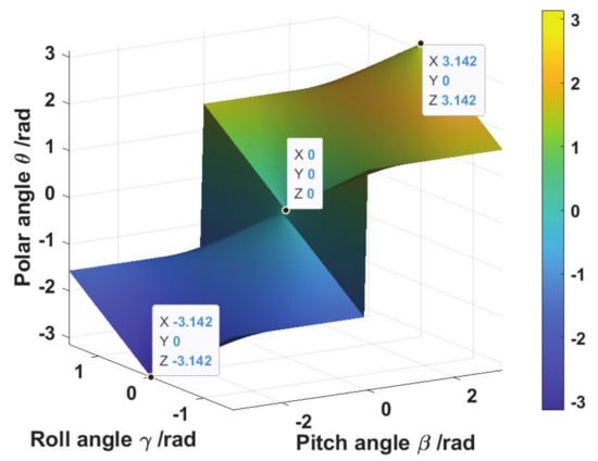
Figure 4. Variationin polar angle $\theta$ with pitch angle $\beta$ and roll angle $\gamma$ of UE.

The variation trends in the proportions of the diffuse component to the total RSS from Tx1, Tx2, Tx3, and Tx4 to UE1 (0, 0, 0.85), UE2 (−1.5, −1.5, 0.85), and UE3 (−2.3, −2.3, 0.85) in response to variations in the polar and yaw angles are illustrated in Figure 5a–c. We find that when the polar angle $\theta$ is greater than $45°$, the received RSS is basically a diffuse component; therefore, the variation range of the x-axis in Figure 5 is set to $0°$–$45°$. When the yaw angle $\alpha$ values are $0°$, $30°$, and $60°$, the diffuse component in the total RSS from Tx1, Tx2, Tx3, and Tx4 to position (0, 0, 0.85) varies slightly with the increase in $\theta$. However, when the polar angle $\theta$ is at its minimum, the proportion of the diffusion component from Tx2, Tx3, and Tx4 is greater than $20\%$. When the polar angle $\theta$ reaches its maximum, the proportion of the diffusion component is close to $50\%$. At position (−1.5, −1.5, 0.85), the proportion of the diffuse component from Tx1 changes slightly with the yaw angle $\alpha$ at approximately $18\%$. The proportions of Tx2, Tx3, and Tx4 are more than $30\%$ and increase rapidly with an increase in $\theta$. At position (−2.3, −2.3, 0.85), the change trend is similar to that at position (−1.5, −1.5, 0.85). With the change in $\theta$, the proportion of the diffuse component increases more significantly, and the maximum proportion can reach $100\%$. Furthermore, when the polar angle $\theta$ is 0–0.1, the proportion of the diffuse component at the three receiving positions remains essentially constant as the yaw angle $\alpha$ changes. When the polar angle $\theta$ increases, the proportion of the diffuse component varies with the change in the receiving position, indicating that the UE rotation around the x-axis has a minor impact on the diffuse component when the polar angle $\theta$ is small. When the polar angle $\theta$ is large, the influence of the yaw angle $\alpha$ on the diffuse component is related to the receiving position. It can be seen that at the same position, the proportion of the diffuse component in RSS from different transmitters is related to the polar and azimuth angles. These two angles have an impact on the incident angle, which is presented in Equations (3) and (8).

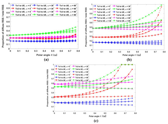
Figure 5. Variation in the proportion of diffuse RSS to total RSS from Tx1, Tx2, Tx3, and Tx4 to UE1, UE2, and UE3 with polar and yaw angles. (a) Tx1, Tx2, Tx3, and Tx4 to UE1 (0, 0, 0.85); (b) Tx1, Tx2, Tx3, and Tx4 to UE2 (−1.5, −1.5, 0.85); (c) Tx1, Tx2, Tx3, and Tx4 to UE3 (−2.3, −2.3, 0.85).

During the trilateral positioning process, the diffuse component cannot be ignored and must be removed from the total RSS. Only after obtaining the pure LOS RSS can an accurate distance estimation using the distance model given by Equation (2) be performed. At present, there is no closed analytic expression for characterizing the diffuse channel impulse response when considering the transmitter and receiver positions and orientations. Thus, obtaining the diffuse channel gain $H_{\mathrm{DIFF}}\left(0\right)$ is vital to obtaining an accurate distance between the Tx and UE.

3. VLC-Based RSS Positioning System

3.1. Optical OFDM–TDMA Positioning Model

The orthogonal frequency division multiplexing (OFDM) transmission technique can be combined with the time division multiple access (TDMA) technique for a multi-user system [27]. The optical OFDM–TDMA (O-OFDM–TDMA) system can be adopted for RSS positioning, in which all subcarriers can be allocated only to a single Tx for the duration of several O-OFDM symbols, as depicted in Figure 6.

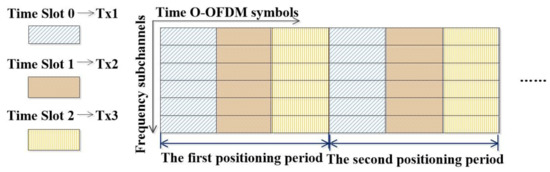
Figure 6. O-OFDM–TDMA RSS positioning model.

In this case, the resource among the Txs is orthogonal in time. The signal frame structure of each Tx is illustrated in Figure 7 within the assigned time slot, which contains two O-OFDM symbols. The first O-OFDM symbol consists of a training symbol; it is used for symbol synchronization in the receiver to determine the initial position of the O-OFDM symbol. The second O-OFDM symbol, with pilot tones at all subcarriers, is transmitted on a regular basis for channel estimation along the time axis. The data symbols, including positioning information, such as LED identification, coordinates of the LED, and transmitted optical power, are inserted into the residual subcarriers. These two consecutive O-OFDM symbols have an identical length of N. The cyclic prefix (CP) is the guard interval inserted between two consecutive O-OFDM symbols to deal with the inter-symbol interference (ISI) over the multipath channel. The length of the CP is $N_{\mathrm{g}}$.

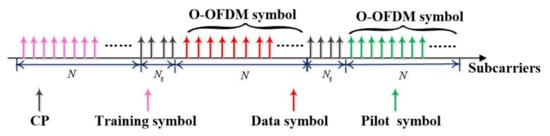
Figure 7. Signal frame structure of each Tx.

3.2. VLC-Based DCO–OFDM Transmission Strategy

We considered the direct current biased O-OFDM (DCO-OFDM) as the transmission strategy because of its high the spectrum and energy efficiencies. A schematic of the DCO–OFDM VLC system is shown in Figure 8. After serial-to-parallel (S/P) conversion, the input data are modulated by an M-ary QAM at the transmitter, resulting in a set of data symbols with length N. We adopted the Zadoff–Chu sequence as the pilot symbol. The lengths of the pilot symbols were identical to those of the data symbols. Because of the intensity modulation and direct detection (IM/DD) of the optical channel, the transmit signal must not only be non-negative but also real-valued. To ensure that the output signal of the inverse fast Fourier transform (IFFT) is a real-valued signal, the IFFT input symbols with length of $2N$ should satisfy the Hermitian symmetry:

$$X_{2N-i}=X_i^{\ast },i=1,2,\dots ,N-1,$$

(11)

where $X_i$ is the signal of the ith subcarrier, which should be $X_0=X_N=0$ to block the DC component. Without loss of generality, we can assume that $\mathrm{E}\left\{\right|X_i{|}^2\}=1$. After an IFFT operation on the Hermitian symmetry symbols, the real-valued time-domain output signal $x_k$ is obtained.

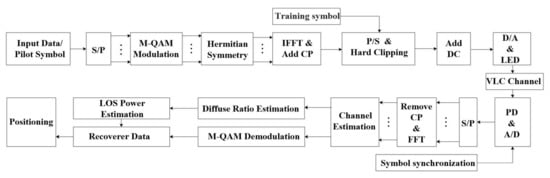
Figure 8. Schematic diagram of a DCO–OFDM VLC system.

The clipping operator is applied to guarantee that the VLC signal is non-negative. The clipped signal $x_{\mathrm{clip},k}$ is achieved by clipping the time-domain signal $x_k$ at the level of $-I_{\mathrm{dc}}$, where $I_{\mathrm{dc}}$ is the DC bias, and the clipping operator is defined as [28]:

$$x_{\mathrm{clip},k}=\left\{\begin{array}{c}{x}_k{x}_k\ge -I_{\mathrm{dc}},\hfill \\ -I_{\mathrm{dc}}{x}_k<-I_{\mathrm{dc}}.\hfill \end{array}\right.$$

(12)

Then, $x_{\mathrm{clip},k}$ is added to $I_{\mathrm{dc}}$, which only affects the 0th subcarrier in the frequency domain. Thus, the non-negative signal can be written as:

$$x_{\mathrm{dc},k}=x_{\mathrm{clip},k}+I_{\mathrm{dc}}.$$

(13)

To avoid the clipping noise caused by the inherent characteristics of the LED, the amplitude of the time-domain signal $x_k$ should be bounded to avoid the clipping operation, and an appropriate DC bias $I_{\mathrm{dc}}$ should satisfy:

$$x_k+I_{\mathrm{dc}}\ge \min \left\{x_k\right\}+I_{\mathrm{dc}}\ge 0.$$

(14)

The digital signal $x_{\mathrm{dc},k}$ is converted to an analog signal $x\left(t\right)$ via a digital-to-analog (D/A) converter and then transmitted by the LED to the indoor channel.

The analog electrical signal received by the photodetector (PD) is given by:

$$\begin{array}{cc}\hfill I_{\mathrm{r}}& =\gamma ·P_{\mathrm{rOpt}}+w\hfill \\ \hfill & =\gamma ·\left[H_{\mathrm{LOS}}\left(0\right)+H_{\mathrm{DIFF}}\left(0\right)\right]P_{\mathrm{t}}+w,\hfill \end{array}$$

(15)

where $\gamma$ denotes the responsivity of the PD, w is the additive white Gaussian noise (AWGN) with zero mean, and its electrical domain power is given by:

$${\sigma }^2={\sigma }_{\mathrm{shot}}^2+{\sigma }_{\mathrm{thermal}}^2,$$

(16)

where ${\sigma }_{\mathrm{shot}}^2$ is the shot noise variance and ${\sigma }_{\mathrm{thermal}}^2$ is the thermal noise variance, which are given by Equations (17) and (18), respectively.

$${\sigma }_{\mathrm{shot}}^2=2q\gamma P_{\mathrm{rOpt}}B+2q{I}_{\mathrm{bg}}{I}_{2}B,$$

(17)

$${\sigma }_{\mathrm{thermal}}^2=\frac{8\pi k{T}_{\mathrm{k}}}{G}\eta A_{\mathrm{PD}}{I}_2{B}^2,+\frac{16{\pi }^{2}k{T}_{\mathrm{k}}\Gamma }{g_{\mathrm{m}}}{\eta }^2{A}_{\mathrm{PD}}^2{I}_3{B}^3,$$

(18)

where q is the electrical charge, $P_{\mathrm{rOpt}}$ denotes the total received optical power, B is the equivalent noise bandwidth, $I_{\mathrm{bg}}$ is the background light current, $I_2$ and $I_3$ are the noise bandwidth factors, k is the Boltzmann’s constant, $T_{\mathrm{k}}$ is the circuit absolute temperature, G represents the open-loop voltage gain, $\eta$ indicates the fixed capacitance per unit area of PD, and $\Gamma$ and $g_{\mathrm{m}}$ denote the field effect transistor (FET) channel noise factor and FET transconductance, respectively.

After filtering out the noise power, based on Equations (2) and (15), the distance from the LED to the UE can be estimated by:

$$d=\sqrt{\frac{P_{\mathrm{t}}(m+1)A_{\mathrm{PD}}}{2\pi ({\widehat{P}}_{\mathrm{rOpt}}-P_{\mathrm{rDIFF}})}{cos}^m\left(\varphi \right)cos\left(\psi \right)T\left(\psi \right)G\left(\psi \right)},$$

(19)

where ${\widehat{P}}_{\mathrm{rOpt}}$ is the measured total optical power given by $\frac{{\widehat{I}}_{\mathrm{r}}}{\gamma }$; $P_{\mathrm{rDIFF}}$ is $H_{\mathrm{DIFF}}\left(0\right)P_{\mathrm{t}}$.

3.3. Diffuse Component Elimination

The digital signal was obtained using an analog-to-digital (A/D) converter. Subsequently, symbol timing synchronization was performed to detect the starting position of the OFDM symbol. Then, pilot symbols and positioning information can be extracted correctly from the received signal.

The frequency domain expression of the received signal $Y_i$ at the ith subcarrier can be expressed as Equation (20) after removing the CP and performing an FFT operation on the digital signal.

$$Y_i=\gamma ·H_{\mathrm{total},i}{X}_i+Z_i,i=1,2,\cdots ,N-1,$$

(20)

The received pilot symbol vector can be given as:

$${\mathbf{Y}}^{\mathrm{p}}=\left[Y_0,Y_1,Y_2,\cdots ,Y_{N-2},Y_{N-1}\right].$$

(21)

The least-squares channel estimation method is applied to estimate the channel frequency response. The LS channel estimation is given by:

$${\widehat{\mathbf{H}}}_{\mathrm{total}}^{\mathit{LS}}={\left({\mathbf{X}}^{\mathrm{p}}\right)}^{-1}{\mathbf{Y}}^{\mathrm{p}}.$$

(22)

where ${\mathbf{X}}^{\mathrm{p}}$ denotes transmitted pilot symbol vector. We denote each component of the estimated channel vector ${\widehat{\mathbf{H}}}_{\mathrm{total}}^{\mathit{LS}}$ by ${\widehat{H}}_{\mathrm{total}}^{\mathit{LS}},k=0,1,2,\cdots ,N-1$. Because each component in ${\mathbf{X}}^{\mathrm{p}}$ is orthogonal, the LS channel estimation ${\widehat{\mathbf{H}}}_{\mathrm{total}}^{\mathit{LS}}$ can be written for each subcarrier as:

$${\widehat{H}}_{\mathrm{total}}^{\mathit{LS}}\left[k\right]=\frac{Y\left[k\right]}{X\left[k\right]},k=0,1,2,\cdots ,N-1.$$

(23)

The total channel gain ${\widehat{H}}_{\mathrm{total}}^{\mathit{LS}}\left[k\right]$ for each subcarrier contains two parts: LOS gain and diffuse gain. By performing a length of $2N$ IFFT on the estimated channel vector ${\widehat{\mathbf{H}}}_{\mathrm{total}}^{\mathit{LS}}$, the time-domain discrete impulse response $\widehat{h}\left(n\right)$ can be obtained. Theoretically, $\widehat{h}\left(0\right)$ represents the LOS channel gain $H_{\mathrm{LOS}}\left(0\right)$. The number of channel paths is vital for determining the proportion of LOS gain to the total gain. Parseval’s theorem states that the total energy of the a signal in the time domain is equal to the total energy of the signal in the frequency domain.

Subtraction of ${\sum }_{n=0}^l{\left|\widehat{h}\left(n\right)\right|}^2$ and ${\sum }_{n=0}^{l+1}{\left|\widehat{h}\left(n\right)\right|}^2$ from the frequency domain total power yields the power $P_l$ and $P_{l+1}$, respectively. If $P_l$ minus $P_{l+1}$ is less than or equal to a certain value, $\delta$, then l is the last multipath channel. Theoretically, the total number of channel paths is $L=l+1$. Because the multipath gain has little influence on the proportion of the diffuse component when it is less than ${10}^{-10}$, the value of $\delta$ is set to ${10}^{-20}$. The number of channel paths is determined in accordance with the steps described in Algorithm 1.

Algorithm 1 Estimation of number of channel paths based on Parseval’s theorem

1: Perform an IFFT operation on the estimated channel vector ${\widehat{\mathbf{H}}}_{\mathrm{total}}^{\mathit{LS}}$; 2: Calculate the frequency domain total power $P_{\mathrm{f}}$ based on the estimated channel vector ${\widehat{\mathbf{H}}}_{\mathrm{total}}^{\mathit{LS}}$; $$P_{\mathrm{f}}=\frac{1}{2N}\sum _{k=0}^{2N-1}{\left|{\widehat{H}}_{\mathrm{total}}^{\mathit{LS}}\left[k\right]\right|}^2;$$ (24) 3: Perform the subtraction of ${\sum }_{n=0}^l{\left|\widehat{h}\left(n\right)\right|}^2$ from $P_{\mathrm{f}}$ to obtain $P_l$; $$P_l=P_{\mathrm{f}}-\sum _{n=0}^l{\left|\widehat{h}\left(n\right)\right|}^2;$$ (25) 4: Perform the subtraction of ${\sum }_{n=0}^{l+1}{\left|\widehat{h}\left(n\right)\right|}^2$ from $P_{\mathrm{f}}$ to obtain $P_{l+1}$, $$P_{l+1}=P_{\mathrm{f}}-\sum _{n=0}^{l+1}{\left|\widehat{h}\left(n\right)\right|}^2;$$ (26) 5: If $P_l-P_{l+1}\le \delta$ is satisfied; l is the last multipath channel. $L=l+1$ is the actual number of channel paths.

According to the estimated number of channel paths, the proportion of the diffuse channel gain to the total channel gain is expressed as:

$$\widehat{\eta }=1-\frac{\widehat{h}\left(0\right)}{{\sum }_{n=0}^{L-1}\widehat{h}\left(n\right)}.$$

(27)

The distances between different Txs to UE can be obtained by replacing the term ${\widehat{P}}_{\mathrm{rOpt}}-P_{\mathrm{rDIFF}}$ in Equation (19) with ${\widehat{P}}_{\mathrm{rLOS}}$ given in Equation (28).

$${\widehat{P}}_{\mathrm{rLOS}}={\widehat{P}}_{\mathrm{rOpt}}·\left(1-\widehat{\eta }\right).$$

(28)

3.4. Position Estimation

Based on Equations (19) and (28), the distances between the LEDs and UE, denoted as $d_1$, $d_2$, and $d_3$, can be estimated by solving the set of equations:

$$\left\{\begin{array}{cc}\hfill d_1^{m+3}& =\frac{P_t(m+1)A_{\mathrm{PD}}{T}_{\mathrm{s}}G}{2\pi {\widehat{P}}_{\mathrm{rLOS},1}}\{h^{m}sin\theta \left[(x_1-x_{\mathrm{u}})cos\omega +(y_1-y_{\mathrm{u}})sin\omega \right]+h^{m+1}cos\theta \},\hfill \\ \hfill d_2^{m+3}& =\frac{P_t(m+1)A_{\mathrm{PD}}{T}_{\mathrm{s}}G}{2\pi {\widehat{P}}_{\mathrm{rLOS},2}}\{h^{m}sin\theta \left[(x_2-x_{\mathrm{u}})cos\omega +(y_2-y_{\mathrm{u}})sin\omega \right]+h^{m+1}cos\theta \},\hfill \\ \hfill d_3^{m+3}& =\frac{P_t(m+1)A_{\mathrm{PD}}{T}_{\mathrm{s}}G}{2\pi {\widehat{P}}_{\mathrm{rLOS},3}}\{h^{m}sin\theta \left[(x_3-x_{\mathrm{u}})cos\omega +(y_3-y_{\mathrm{u}})sin\omega \right]+h^{m+1}cos\theta \}.\hfill \end{array}\right.$$

(29)

The distances $d_1$, $d_2$, and $d_3$ can also be expressed as follows:

$$\left\{\begin{array}{cc}\hfill d_1^2& ={(x_{\mathrm{u}}-x_1)}^2+{(y_{\mathrm{u}}-y_1)}^2+h^2,\hfill \\ \hfill d_2^2& ={(x_{\mathrm{u}}-x_2)}^2+{(y_{\mathrm{u}}-y_2)}^2+h^2,\hfill \\ \hfill d_3^2& ={(x_{\mathrm{u}}-x_3)}^2+{(y_{\mathrm{u}}-y_3)}^2+h^2.\hfill \end{array}\right.$$

(30)

Based on the linear least square (LLS) estimator, $x_{\mathrm{u}}$ and $y_{\mathrm{u}}$ can be expressed as:

$$\left[\begin{array}{c}{x}_{\mathrm{u}}\\ y_{\mathrm{u}}\end{array}\right]={\left[A^{\mathrm{T}}A\right]}^{-1}{A}^{\mathrm{T}}B.$$

(31)

where

$$A=\left[\begin{array}{cc}{x}_2-x_1& y_2-y_1\\ x_3-x_1& y_3-y_1\end{array}\right],$$

$$B=\left[\begin{array}{c}\frac{1}{2}(d_1^2-d_2^2-x_1^2+x_2^2-y_1^2+y_2^2)\\ \frac{1}{2}(d_1^2-d_3^2-x_1^2+x_3^2-y_1^2+y_3^2)\end{array}\right].$$

From Equation (31), it can be seen that $x_{\mathrm{u}}$ and $y_{\mathrm{u}}$ can be represented by $x_1$, $x_2$, $x_3$, $y_1$, $y_2$, $y_3$, $d_1$, $d_2$, and $d_3$, where $x_1$, $x_2$, $x_3$, $y_1$, $y_2$, and $y_3$ are the coordinates of the three positioning LEDs, which can be obtained from the positioning information. Therefore, $x_{\mathrm{u}}$ and $y_{\mathrm{u}}$ can actually be expressed as $x_{\mathrm{u}}=f(d_1,d_2,d_3)$ and $y_{\mathrm{u}}=f(d_1,d_2,d_3)$. Bringing $x_{\mathrm{u}}=f(d_1,d_2,d_3)$ and $y_{\mathrm{u}}=f(d_1,d_2,d_3)$ into Equation (29), they become quartic equations of $d_1$, $d_2$, and $d_3$ by performing the Gaussian elimination method on quartic equations about $d_1$. At the same time, $d_2^4$ and $d_3^4$ are represented by $d_1^4$. The quartic equation of $d_1$ can be solved by a bisection algorithm to obtain $d_1$. Based on the relationship between $d_2^4$, $d_3^4$, and $d_1^4$, $d_2$ and $d_3$ can be solved using $d_1$. Ultimately, bringing $x_1$, $x_2$, $x_3$, $y_1$, $y_2$, $y_3$, $d_1$, $d_2$, and $d_3$ into Equation (31), we can obtain $x_{\mathrm{u}}$ and $y_{\mathrm{u}}$.

4. Cramér–Rao Low Bound on Positioning Estimation Error

The positioning error distribution performance of the UE is limited to the CRLB. By deriving the CRLB of UE, the best theoretical positioning performance with the current environmental parameters can be obtained, which provides a comparison standard for the performance of the positioning methods proposed in this paper.

According to Equations (19) and (28), the received LOS optical power of UE is given by Equation (32), where $P_{\mathrm{t},i}$ is the transmitted optical power of the ith LED, $l_i$ is the distance from the projection of the LED on the receiving surface to UE, and $n_i$ is the AWGN.

$$P_{\mathrm{rLOS},i}\left(l_i\right)=\frac{P_{\mathrm{t},i}\left(m+1\right)A_{\mathrm{PD}}}{2\pi \left(l_i^2+h^2\right)}cos{\left({\varphi }_i\right)}^{m}cos\left({\psi }_i\right)T_{\mathrm{s}}G+n_i,i=1,2,3,4,$$

(32)

As $cos{\varphi }_i=\frac{h}{\sqrt{l_i^2+h^2}}$, $cos{\psi }_i=\frac{(x_i-x_{\mathrm{u}})sin\theta sin\omega +(y_i-y_{\mathrm{u}})sin\theta sin\omega }{\sqrt{l_i^2+h^2}}$, and $i=1,2,3,4$, the received LOS optical power $P_{\mathrm{rLOS},i}$ can be given by Equation (33).

$$P_{\mathrm{rLOS},i}\left(l_i\right)=\frac{P_{\mathrm{t},i}(m+1)A_{\mathrm{PD}}{T}_{\mathrm{s}}G}{2\pi (l_i^2+h^2)}{\left(\frac{h}{\sqrt{l_i^2+h^2}}\right)}^m\frac{(x_i-x_{\mathrm{u}})sin\theta sin\omega +(y_i-y_{\mathrm{u}})sin\theta sin\omega }{\sqrt{l_i^2+h^2}}+n_i.$$

(33)

where $i=1,2,3,4$. Assuming the first term of Equation (33) is $f_i\left(l_i\right)$, we have:

$$P_{\mathrm{rLOS},i}\left(l_i\right)=f_i\left(l_i\right)+n_i,i=1,2,3,4.$$

(34)

Let vectors $\mathit{f}\left(\mathit{l}\right)$ and $\mathit{n}$ be denoted by: $\mathit{f}\left(\mathit{l}\right)=\left[\begin{array}{c}{f}_1\left(l_1\right)\\ f_2\left(l_2\right)\\ f_3\left(l_3\right)\\ f_4\left(l_4\right)\end{array}\right]$, $\mathit{n}=\left[\begin{array}{c}{n}_1\\ n_2\\ n_3\\ n_4\end{array}\right]$.

Then, we have:

$$\frac{\partial \mathit{f}\left(\mathit{l}\right)}{\partial {\mathit{l}}^{\mathrm{T}}}=\left[\begin{array}{cccc}\frac{\partial f_1\left(l_1\right)}{\partial l_1}& \frac{\partial f_1\left(l_1\right)}{\partial l_2}& \frac{\partial f_1\left(l_1\right)}{\partial l_3}& \frac{\partial f_1\left(l_1\right)}{\partial l_4}\\ \frac{\partial f_2\left(l_2\right)}{\partial l_1}& \frac{\partial f_2\left(l_2\right)}{\partial l_2}& \frac{\partial f_2\left(l_2\right)}{\partial l_3}& \frac{\partial f_2\left(l_2\right)}{\partial l_4}\\ \frac{\partial f_3\left(l_3\right)}{\partial l_1}& \frac{\partial f_3\left(l_3\right)}{\partial l_2}& \frac{\partial f_3\left(l_3\right)}{\partial l_3}& \frac{\partial f_3\left(l_3\right)}{\partial l_4}\\ \frac{\partial f_4\left(l_4\right)}{\partial l_1}& \frac{\partial f_4\left(l_4\right)}{\partial l_2}& \frac{\partial f_4\left(l_4\right)}{\partial l_3}& \frac{\partial f_4\left(l_4\right)}{\partial l_4}\end{array}\right].$$

(35)

If $i\ne j$ is satisfied, $\frac{\partial f_i\left(l_i\right)}{\partial l_j}=0$. Then, $\frac{\partial \mathit{f}\left(\mathit{l}\right)}{\partial {\mathit{l}}^{\mathrm{T}}}$ is a diagonal matrix, which can be written as Equation (36), where $\mathrm{\Delta }=-\frac{(m+1)(m+3)A_{\mathrm{PD}}{T}_{\mathrm{s}}G{h}^m}{2\pi }$, and ${\mathrm{\Lambda }}_i=(x_i-x_{\mathrm{u}})sin\theta sin\omega +(y_i-y_{\mathrm{u}})sin\theta sin\omega +hcos\theta ;i=1,2,3,4$.

$$\frac{\partial \mathit{f}\left(\mathit{l}\right)}{\partial {\mathit{l}}^{\mathrm{T}}}=\mathrm{\Delta }\mathrm{diag}\left[\frac{P_{\mathrm{t},1}{l}_1{\mathrm{\Lambda }}_1}{{(l_1^2+h^2)}^{\frac{m+5}{2}}},\frac{P_{\mathrm{t},2}{l}_2{\mathrm{\Lambda }}_2}{{(l_2^2+h^2)}^{\frac{m+5}{2}}},\frac{P_{\mathrm{t},3}{l}_3{\mathrm{\Lambda }}_3}{{(l_3^2+h^2)}^{\frac{m+5}{2}}},\frac{P_{\mathrm{t},4}{l}_4{\mathrm{\Lambda }}_4}{{(l_4^2+h^2)}^{\frac{m+5}{2}}}\right].$$

(36)

Additionally, the following relationships are satisfied:

$$\left\{\begin{array}{cc}\hfill l_1^2& ={(x_{\mathrm{u}}-x_1)}^2+{(y_{\mathrm{u}}-y_1)}^2,\hfill \\ \hfill l_2^2& ={(x_{\mathrm{u}}-x_2)}^2+{(y_{\mathrm{u}}-y_2)}^2,\hfill \\ \hfill l_3^2& ={(x_{\mathrm{u}}-x_3)}^2+{(y_{\mathrm{u}}-y_3)}^2,\hfill \\ \hfill l_4^2& ={(x_{\mathrm{u}}-x_4)}^2+{(y_{\mathrm{u}}-y_4)}^2.\hfill \end{array}\right.$$

(37)

Let $\mathit{X}=\left[\begin{array}{c}{x}_{\mathrm{u}}\\ y_{\mathrm{u}}\end{array}\right]$; we have:

$$\frac{\partial \mathit{l}}{\partial {\mathit{X}}^{\mathrm{T}}}=\left[\begin{array}{cc}\frac{\partial l_1}{\partial x_{\mathrm{u}}}& \frac{\partial l_1}{\partial y_{\mathrm{u}}}\\ \frac{\partial l_2}{\partial x_{\mathrm{u}}}& \frac{\partial l_2}{\partial y_{\mathrm{u}}}\\ \frac{\partial l_3}{\partial x_{\mathrm{u}}}& \frac{\partial l_3}{\partial y_{\mathrm{u}}}\\ \frac{\partial l_4}{\partial x_{\mathrm{u}}}& \frac{\partial l_4}{\partial y_{\mathrm{u}}}\end{array}\right]=\left[\begin{array}{cc}\frac{x_{\mathrm{u}}-x_1}{l_1}& \frac{y_{\mathrm{u}}-y_1}{l_1}\\ \frac{x_{\mathrm{u}}-x_2}{l_2}& \frac{y_{\mathrm{u}}-y_2}{l_2}\\ \frac{x_{\mathrm{u}}-x_3}{l_3}& \frac{y_{\mathrm{u}}-y_3}{l_3}\\ \frac{x_{\mathrm{u}}-x_4}{l_4}& \frac{y_{\mathrm{u}}-y_4}{l_4}\end{array}\right].$$

(38)

The CRLB of position error is given by:

$$\mathit{B}\left(\mathit{X}\right)={\left[{\left(\frac{\partial \mathit{f}\left(\mathit{l}\right)}{\partial {\mathit{X}}^{\mathrm{T}}}\right)}^{\mathrm{T}}{\mathit{Q}}^{-1}\frac{\partial \mathit{f}\left(\mathit{l}\right)}{\partial {\mathit{X}}^{\mathrm{T}}}\right]}^{-1},$$

(39)

where $\mathit{Q}$ indicates noise covariance matrix, $\mathit{Q}=\mathit{E}\left[\mathit{n}{\mathit{n}}^{\mathrm{T}}\right]$. According to the chain rule, we have $\frac{\partial \mathit{f}\left(\mathit{l}\right)}{\partial {\mathit{X}}^{\mathrm{T}}}=\frac{\partial \mathit{f}\left(\mathit{l}\right)}{\partial {\mathit{l}}^{\mathrm{T}}}\frac{\partial \mathit{l}}{\partial {\mathit{X}}^{\mathrm{T}}}$.

By combining Equations (36) and (38), we obtain:

$$\frac{\partial \mathit{f}\left(\mathit{l}\right)}{\partial {\mathit{X}}^{\mathrm{T}}}=\mathrm{\Delta }\left[\begin{array}{cc}\frac{P_{\mathrm{t},1}\left(x_{\mathrm{u}}-x_1\right){\mathrm{\Lambda }}_1}{{\left(l_1^2+h^2\right)}^{\frac{m+5}{2}}}& \frac{P_{\mathrm{t},1}\left(y_{\mathrm{u}}-y_1\right){\mathrm{\Lambda }}_1}{{\left(l_1^2+h^2\right)}^{\frac{m+5}{2}}}\\ \frac{P_{\mathrm{t},2}\left(x_{\mathrm{u}}-x_2\right){\mathrm{\Lambda }}_2}{{\left(l_2^2+h^2\right)}^{\frac{m+5}{2}}}& \frac{P_{\mathrm{t},2}\left(y_{\mathrm{u}}-y_2\right){\mathrm{\Lambda }}_2}{{\left(l_2^2+h^2\right)}^{\frac{m+5}{2}}}\\ \frac{P_{\mathrm{t},3}\left(x_{\mathrm{u}}-x_3\right){\mathrm{\Lambda }}_3}{{\left(l_3^2+h^2\right)}^{\frac{m+5}{2}}}& \frac{P_{\mathrm{t},3}\left(y_{\mathrm{u}}-y_3\right){\mathrm{\Lambda }}_3}{{\left(l_3^2+h^2\right)}^{\frac{m+5}{2}}}\\ \frac{P_{\mathrm{t},4}\left(x_{\mathrm{u}}-x_4\right){\mathrm{\Lambda }}_4}{{\left(l_4^2+h^2\right)}^{\frac{m+5}{2}}}& \frac{P_{\mathrm{t},4}\left(y_{\mathrm{u}}-y_4\right){\mathrm{\Lambda }}_4}{{\left(l_4^2+h^2\right)}^{\frac{m+5}{2}}}\end{array}\right].$$

(40)

The CRLB $\mathit{B}\left(\mathit{X}\right)$ of the UE location estimation error is obtained by substituting Equation (40) into Equation (39).

5. Discussion

In this section, the position performance of different methods is compared and analyzed in the scenario shown in Figure 1. The LLS-based positioning method described in Section 3.4 is the comparison method. The LLS positioning method that uses the total received power is denoted as LLS-1, and the LLS positioning method that uses the LOS power without considering the receiving orientation is denoted as LLS-2. The primary parameters are listed in Table 1. Assuming that the received sample interval is 10 ns, the length of the IFFT is 64, the length of the CP is 8, and the modulation scheme on each subcarrier is 4QAM. The position and receiving orientations of the UE were generated randomly, and the positioning result was the average of 1000 iterations.

The average error (AE) and root mean square error (RMSE) of position estimation are used for evaluating positioning accuracy. When the AE is the same, the greater the deviation between the estimated position and the actual position, the higher the dispersion of the error, and the greater the RMSE. The definitions of AE and RMSE are as follows:

$$\mathrm{AE}=\frac{1}{N}\sum _{i=1}^N\sqrt{[{(x_i-x_{\mathrm{u}})}^2+{(y_i-y_{\mathrm{u}})}^2]}$$

(41)

$$\mathrm{RMSE}=\sqrt{\frac{1}{N}{\sum }_{i=1}^N[{(x_i-x_{\mathrm{u}})}^2+{(y_i-y_{\mathrm{u}})}^2]}$$

(42)

The AE of our proposed method is 4.9 cm at an SNR of 30 dB. In the scheme presented in [24], when the dataset size is ${10}^5$, the AEs based on the convolutional neural network (CNN), the multiple layer perceptron (MLP), and K-nearest neighbor (KNN) are 14.55 cm, 15.05 cm, and 27.30 cm, respectively. When the dataset size is ${10}^6$, although the AEs based on CNN, MLP, and KNN descend to 10.53 cm, 13.04 cm, and 17.34 cm, respectively, they are still higher than our proposed method The RMSEs of positioning estimation based on the proposed method, LLS-1, and LLS-2 are 5.2 cm, 80.4 cm, and 463.1 cm at an SNR of 30 dB, respectively. Because the error between the estimated LOS power and actual LOS power is very small at a high SNR, the RMSE of the proposed method is the smallest. For LLS-1, the total power received includes the diffuse component introduced by the reflective link, resulting in a total power received that is greater than the actual LOS power. This power deviation between the received total power and actual LOS power makes the estimated distance between the LED and UE smaller than the actual distance. As a result, the RMSE is larger than the proposed scheme. Considering LLS-2, according to Equation (3), the incidence angle ${\varphi }_0$ of the optical signal will change when the receiving orientation is nonzero. Compared with vertical receiving, ${\varphi }_0$ becomes larger or smaller, depending on the polar and azimuth angles, in addition to the UE location. When ${\varphi }_0$ becomes larger, the received optical power decreases compared with the vertical receiving, and the estimated distance between the LED and UE based on this power is larger than the actual distance. Conversely, when ${\varphi }_0$ becomes smaller, the received optical power increases compared with the vertical receiving, and the estimated distance between the LED and UE is smaller than the actual distance. Consequently, the estimated position is wildly inaccurate. Thus, the RMSE is also larger than the proposed method.

The cumulative distribution functions (CDFs) of the positioning error based on the proposed method, LLS-1, and LLS-2 at an SNR of 30 dB are presented in Figure 9. It is observed that the estimated position accuracy by adopting the proposed positioning scheme is greater than LLS-1 and LLS-2. The minimum and maximum average error are approximately 3 cm and 8 cm, respectively. The minimum average error of LLS-1 is identical to the proposed scheme. However, The maximum average error is approximately 1.2 m. If the UE is considered to be received vertically, that is, without considering the actual receiving orientation of the UE, the minimum average position error based on LLS-2 is very large and can reach to 50 cm, even when the estimated LOS power accuracy is very high.

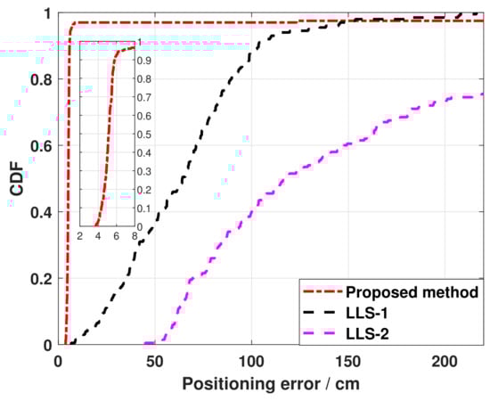
Figure 9. CDFs of the positioning error at an SNR of 30 dB.

Considering the actual receiving orientation of the UE, Figure 10 compares the indoor localization error distribution based on the proposed method and LLS-1 at an SNR of 30 dB. It can be seen that at the center of the room, the localization errors are close in both cases; the localization errors estimated based on LLS-1 at the other locations are larger than those estimated based on the proposed method. This can be explained as follows: at the center of the room, influenced by the receiving orientation, even if the LOS power changes compared to the vertical orientation, provided that the LED is within the FOV of the UE, the proportion of LOS power is considerably larger than the proportion of diffuse power, and the deviation of the total received power from the LOS power is smaller; therefore, the difference in the positioning error between the two cases is not significant. Approaching from the center of the room to the corner, the proportion of LOS power from one or two LEDs is always considerably smaller than the proportion of diffuse power, resulting in a larger positioning error.

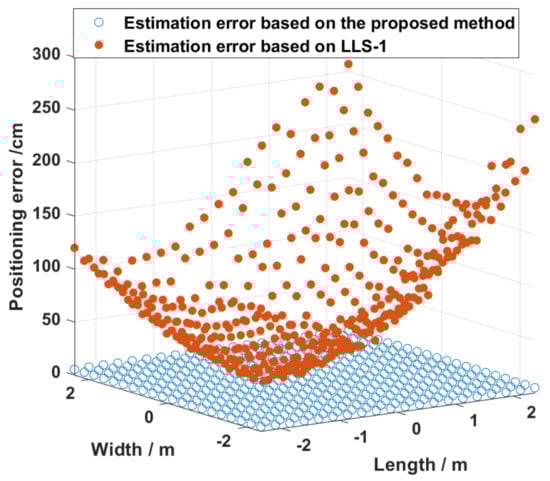
Figure 10. Comparison of positioning error distribution at an SNR of 30 dB.

The CDF of the localization error obtained using the proposed method for different SNRs is shown in Figure 11. It can be observed that the larger the SNR, the smaller the maximum positioning error that can be achieved throughout the room. The maximum localization errors are approximately 3, 8, 10, 15, and 20 cm for SNRs of 45, 40, 35, 30, and 25 dB, respectively, with the current environmental parameters. This is because the higher the SNR, the higher the channel estimation accuracy, the closer the estimated LOS power to the actual LOS power, and the higher the localization accuracy.

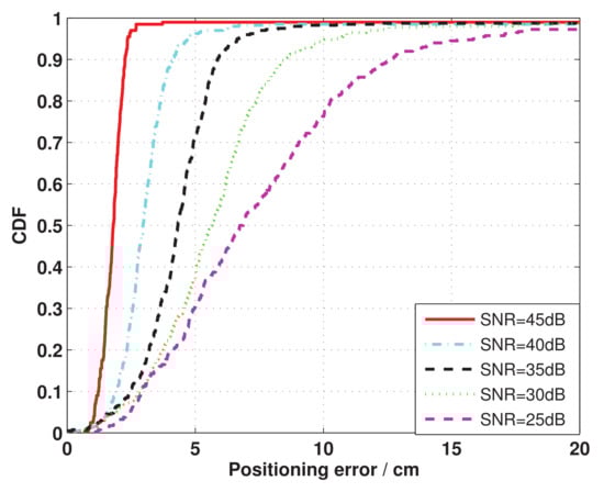
Figure 11. CDFs of the positioning error based on the proposed method at different SNRs.

Figure 12 shows the indoor CRLB distribution estimated using Equation (39) at an SNR of 25 dB, where the receiving orientation at each position is randomly generated. It is assumed that the background noise is certain and that the LED is located within the FOV of the UE. Then, the larger the share of diffuse power in the total received power at the same received position, the larger the power deviation, the larger the caused positioning deviation, and the larger the total positioning error.

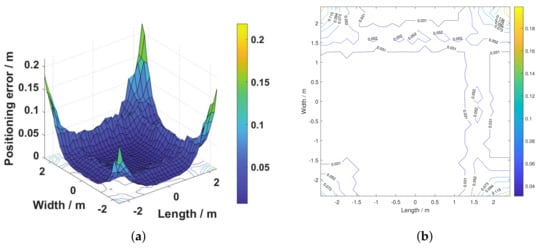
Figure 12. CRLB distribution. (a) Three-dimensional map; (b) contour map.

Figure 13a–c show the trend in positioning error versus the CRLB at different SNRs for positions UE1 $(-0.5,-0.5,0.85)$ with an azimuth angle $\omega$ of $31\pi /18$ and a polar angle $\theta$ of $2\pi /9$, UE2 $(-1.5,-1.5,0.85)$ with an azimuth angle $\omega$ of $34\pi /18$ and a polar angle $\theta$ of $2\pi /9$, and UE3 $(-2.4,-2.4,0.85)$ with an azimuth angle $\omega$ of $35\pi /18$ and a polar angle $\theta$ of $2\pi /9$, where the percentage of diffuse power to total received power is $30\%$. As shown in Figure 13, when the SNR is small, the channel estimation error is larger, and the diffuse power induced by the reflective link cannot be completely eliminated. The deviation between the LOS power used to estimate the distance between the LED and UE and the actual LOS power is larger, which causes a larger localization deviation. Therefore, at a low SNR, the localization error is larger and cannot be matched well with the CRLB. As the SNR increases, the channel estimation accuracy improves, and the deviation of the estimated LOS power from the actual received LOS power is small, causing the localization error to converge with the CRLB. This means that the proposed localization method can achieve the best localization performance with the current environmental parameters. It is worth noting that at the corner of the room, although the diffuse power can be effectively removed at a high SNR, the LOS power is smaller, resulting in a larger localization error than UE1 and UE2. In addition, we can observe that the localization errors based on LLS-1 and LLS-2 do not decrease with an increase in SNR, and there is always an error floor, which depends on the receiving position and orientation.

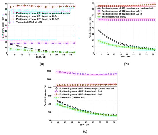
Figure 13. Comparisons of theoretical CRLBs and positioning errors at different positions with varying SNR. (a) UE1 with position (−0.5, −0.5, 0.85), $\omega$ = $31\pi /18$, and $\theta$ = $2\pi /9$, (b) UE2 with position (−1.5, −1.5, 0.85), $\omega$ = $34\pi /18$, and $\theta$ = $2\pi /9$, (c) UE3 with position (−2.4, −2.4, 0.85), $\omega$ = $35\pi /18$, and $\theta$ = $2\pi /9$.

6. Conclusions

In this paper, we proposed a novel trilateration RSS-based approach that can efficiently eliminate diffuse power to infer the position of UE with a random receiving orientation. We found that the proportion of the diffuse component from one or two positioned LEDs varies considerably with the polar and azimuth angles of the UE for the same position, approaching 100% in severe cases. By utilizing the channel estimate method and Parseval’s theorem, we determined the proportion of diffuse power to the total power with a random receiving orientation and used the estimated LOS power to estimate the position of the UE. The simulation results demonstrated that localization accuracy depends on the SNR. The higher the SNR, the higher the channel estimation accuracy, and the smaller the deviation of the estimated LOS power from the actual LOS power, the higher the localization accuracy. At SNRs of 45 and 25 dB, the maximum positioning errors approach 3 cm and 15 cm at the corner of the room with a random receiving orientation, respectively. In addition, even if the deviation of the estimated LOS power from the actual LOS power is small, the localization error remains significant when the receiving orientation of the UE is ignored. By deriving the theoretical CRLB of LOS-based indoor VLP considering receiving orientation, we compared the localization performance of the proposed method with LLS-1, LLS-2, and the CRLB at various SNRs. The results show that the localization error based on the proposed method of all the received positions in the room can reach the theoretical CRLB at approximately 25 dB. However, LLS-1 and LLS-2 cannot achieve the theoretical CRLB even at a high SNR.

References

- Chen, L.; Thombre, S.; Järvinen, K.; Alén-Savikko, A.; Leppäkoski, H.; Bhuiyan, M.Z.H.; Bu-Pasha, S.; Ferrara, G.N.; Honkala, S.; Lindqvist, J.; et al. Robustness, security and privacy in location-based services for future iot: A survey. IEEE Access 2017, 5, 8956–8977. [Google Scholar] [CrossRef]
- Maheepala, M.; Kouzani, A.Z.; Joordens, M.A. Light-based indoor positioning systems: A review. IEEE Sens. J. 2020, 20, 3971–3995. [Google Scholar] [CrossRef]
- Shirehjini, A.A.N.; Shirmohammadi, S. Improving accuracy and robustness in hf-rfid-based indoor positioning with kalman filtering and tukey smoothing. IEEE Trans. Instrum. Meas. 2020, 69, 9190–9202. [Google Scholar] [CrossRef]
- Shao, W.; Luo, H.; Zhao, F.; Tian, H.; Yan, S.; Crivello, A. Accurate indoor positioning using temporal–spatial constraints based on wi-fi fine time measurements. IEEE Internet Things J. 2020, 7, 11006–11019. [Google Scholar] [CrossRef]
- Zhu, X.; Yi, J.; Cheng, J.; He, L. Adapted error map based mobile robot uwb indoor positioning. IEEE Trans. Instrum. Meas. 2020, 69, 6336–6350. [Google Scholar] [CrossRef]
- Fang, S.H.; Wang, C.H.; Huang, T.Y.; Yang, C.H.; Chen, Y.S. An enhanced ZigBee indoor positioning system with an ensemble approach. IEEE Commun. Lett. 2012, 16, 564–567. [Google Scholar] [CrossRef]
- Huang, N.; Gong, C.; Luo, J.; Xu, Z. Design and demonstration of robust visible light positioning based on received signal strength. J. Lightw. Technol. 2020, 38, 5695–5707. [Google Scholar] [CrossRef]
- Hussain, B.; Wang, Y.; Chen, R.; Cheng, H.C.; Yue, C.P. Lidr: Visible-light-communication-assisted dead reckoning for accurate indoor localization. IEEE Internet Things J. 2022, 9, 15742–15755. [Google Scholar] [CrossRef]
- Hong, C.Y.; Wu, Y.C.; Liu, Y.; Chow, C.W.; Yeh, C.H.; Hsu, K.L.; Lin, D.C.; Liao, X.L.; Lin, K.H.; Chen, Y.Y. Angle-of-arrival (AOA) visible light positioning (vlp) system using solar cells with third-order regression and ridge regression algorithms. IEEE Photonics J. 2020, 12, 7902605. [Google Scholar] [CrossRef]
- Keskin, M.F.; Gezici, S.; Arikan, O. Direct and Two-Step Positioning in Visible Light Systems. IEEE Trans. Wirel. Commun. 2018, 66, 239–254. [Google Scholar] [CrossRef]
- Du, P.F.; Chen, C.; Zhong, W.D. Demonstration of a low-complexity indoor visible light positioning system using an enhanced TDOA scheme. IEEE Photonics J. 2018, 10, 7905110. [Google Scholar] [CrossRef]
- Li, Z.P.; Qiu, G.D.; Zhao, L.; Jiang, M. Dual-mode led sided visible light positioning system under multi-path propagation: Design and demonstration. IEEE Trans. Wirel. Commun. 2021, 20, 5986–6003. [Google Scholar] [CrossRef]
- Abou-Shehada, I.M.; AlMuallim, A.F.; AlFaqeh, A.K.; Muqaibel, A.H.; Park, K.H.; Alouini, M.S. Accurate indoor visible light positioning using a modified pathloss model with sparse fingerprints. J. Lightw. Technol. 2021, 39, 6487–6497. [Google Scholar] [CrossRef]
- Alam, F.; Chew, M.T.; Wenge, T.; Gupta, G.S. An accurate visible light positioning system using regenerated fingerprint database based on calibrated propagation model. IEEE Trans. Instrum. Meas. 2019, 68, 2714–2723. [Google Scholar] [CrossRef]
- Wu, Y.C.; Hsu, K.L.; Liu, Y.; Hong, C.Y.; Chow, C.W.; Yeh, C.H.; Liao, X.L.; Lin, K.H.; Chen, Y.Y. Using linear interpolation to reduce the training samples for regression based visible light positioning system. IEEE Photonics J. 2020, 12, 7901305. [Google Scholar] [CrossRef]
- Wang, K.Y.; Liu, Y.J.; Hong, Z.Y. RSS-based visible light positioning based on channel state information. Opt. Express 2022, 30, 5683–5699. [Google Scholar] [CrossRef]
- Bai, L.; Yang, Y.; Feng, C.Y.; Guo, C.L. Received signal strength assisted perspective-three-point algorithm for indoor visible light positioning. Opt. Express 2020, 28, 28045–28095. [Google Scholar] [CrossRef]
- Lee, K.; Park, H.; Barry, J.R. Indoor channel characteristics for visible light communications. IEEE Commun. Lett. 2011, 15, 217–219. [Google Scholar] [CrossRef]
- Gu, W.; Aminikashani, M.; Deng, P.; Kavehrad, M. Impact of multipath reflections on the performance of indoor visible light positioning systems. J. Lightw. Technol. 2016, 34, 2578–2587. [Google Scholar] [CrossRef]
- Wu, N.; Feng, L.; Yang, A. Localization accuracy improvement of a visible light positioning system based on the linear illumination of LED sources. IEEE Photonics J. 2017, 9, 7905611. [Google Scholar] [CrossRef]
- Yang, F.; Gao, J.; Liu, Y. Indoor visible light positioning system based on cooperative localization. Opt. Eng. 2019, 58, 016108. [Google Scholar] [CrossRef]
- Kim, H.S.; Kim, D.R.; Yang, S.H.; Son, Y.H. An indoor visible light communication positioning system using a rf carrier allocation technique. J. Lightw. Technol. 2013, 31, 134–144. [Google Scholar] [CrossRef]
- Soltani, M.D.; Purwita, A.A.; Zeng, Z.; Haas, H.; Safari, M. Modeling the random orientation of mobile devices: Measurement, analysis and lifi use case. IEEE Trans. Commun. 2018, 67, 2157–2172. [Google Scholar] [CrossRef]
- Arfaoui, M.A.; Soltani, M.D.; Tavakkolnia, I.; Ghrayeb, A.; Assi, C.; Safari, M.; Haas, H. Invoking deep learning for joint estimation of indoor lifi user position and orientation. IEEE J. Sel. Area Commun. 2021, 39, 2890–2905. [Google Scholar] [CrossRef]
- Mai, D.H.; Le, H.D.; Pham, T.V.; Pham, A.T. Design and performance evaluation of large-scale vlc-based indoor positioning systems under impact of receiver orientation. IEEE Access 2020, 8, 61891–61904. [Google Scholar] [CrossRef]
- Yin, L.; Wu, X.; Haas, H. Indoor visible light positioning with angle diversity transmitter. In Proceedings of the IEEE 82nd Vehicular Technology Conference, Boston, MA, USA, 6–9 September 2015; pp. 1–5. [Google Scholar]
- Abdelhady, A.M.; Amin, O.; Chaaban, A.; Shihada, B.; Alouini, M.S. Downlink resource allocation for dynamic TDMA-based VLC systems. IEEE Trans. Wirel. Commun. 2019, 18, 108–120. [Google Scholar] [CrossRef]
- Yang, R.X.; Ma, S.H.; Xu, Z.H.; Li, H.; Liu, X.D.; Ling, X.T.; Deng, X.; Zhang, X.; Li, S.Y. Spectral and energy efficiency of DCO-OFDM in visible light communication systems with finite-alphabet inputs. IEEE Trans. Wirel. Commun. 2022, 21, 6018–6032. [Google Scholar] [CrossRef]
Disclaimer/Publisher’s Note: The statements, opinions and data contained in all publications are solely those of the individual author(s) and contributor(s) and not of MDPI and/or the editor(s). MDPI and/or the editor(s) disclaim responsibility for any injury to people or property resulting from any ideas, methods, instructions or products referred to in the content. |
© 2023 by the authors. Licensee MDPI, Basel, Switzerland. This article is an open access article distributed under the terms and conditions of the Creative Commons Attribution (CC BY) license (https://creativecommons.org/licenses/by/4.0/).