Abstract
The so-called arbitrary decomposition of a given Mueller matrix into a convex sum of nondepolarizing constituents provides a general framework for parallel decompositions of polarimetric interactions. Even though arbitrary decomposition can be performed through an infinite number of sets of components, the nature of such components is subject to certain restrictions which limit the interpretation of the Mueller matrix in terms of simple configurations. In this communication, a new approach based on the addition of some portion of a perfect depolarizer before the parallel decomposition is introduced, leading to a set of three components which depend, respectively, on the first column, the first row, and the remaining 3 × 3 submatrix of the original Mueller matrix, so that those components inherit, in a decoupled manner, the polarizance vector, the diattenuation vector, and the combined complementary polarimetric information on depolarization and retardance.
1. Introduction
Mueller polarimetry nowadays has an immense variety of applications in science, engineering, remote sensing, etc. Once a Mueller matrix M is measured, the analysis of the information provided by the sixteen real elements of M constitutes a critical stage, in which different procedures are applied, including the identification of descriptors of diattenuation, polarizance, retardance, and depolarization, as well as methods for the serial and parallel decompositions of M into simpler components. In particular, so-called arbitrary and characteristic decompositions [1,2,3] constitute powerful tools that provide sets of peculiar parallel constituents that are susceptible to specific interpretations.
Nevertheless, the scope of potential components with prescribed features is limited by mathematical restrictions that rely on the fact that the coherency matrix C [4], a positive semidefinite Hermitian matrix that is biunivocally associated with the given M (that is, M determines C unambiguously and vice versa, see Equation (4)), does not always satisfy the property , but its rank can take integer values in the interval [5,6]. Recall that equals the number of independent parallel components of M [1,3].
In this work, a new composition-decomposition approach is presented in which, prior to the application of a specific parallel decomposition, the measured M is combined with a portion of a perfect depolarizer, of which the associated normalized Mueller matrix has the diagonal form [6]. Due to the simple structure of , which corresponds to polarimetric white noise [7], the composed matrix inherits all the anisotropies exhibited by M. Analogously to what occurs in some image diagnostic techniques, where certain contrast agents or colorants are added to the sample in order to improve the images, in the present case, a fully isotropic element is added with the aim of extending the scope of decompositions, which allows certain featured representations to be obtained.
The decompositions dealt with in this communication are focused on identifying sets of three constituents of which the Mueller matrices have the simplest possible structure, regardless of the fact that they are, in general, depolarizing.
The structure of the present communication is organized as follows. The main notions necessary for the development of the new approach are presented in Section 2; Section 3 describes the formulation of the parallel composition of a given Mueller matrix M and a perfect depolarizer; Section 4 deals with the introduction of the homogeneous extended form of M and its decomposition, where the constituents exhibit equal mean intensity coefficients and are analyzed from the mathematical, geometric, and physical points of view; Section 5 describes an alternative extended decomposition of M where the constituents, being of similar nature to those of the homogeneous extended decomposition, exhibit different mean intensity coefficients, and have even simpler forms; Section 6 is devoted to the analysis of the extended decompositions for the particular case in which M lacks either polarizance or diattenuation; and the obtained results are discussed in Section 7.
2. Theoretical Background
The transformation of polarized light by the action of a linear medium (under fixed interaction conditions) can always be represented mathematically as where s and are the Stokes vectors that represent the states of polarization of the incident and emerging light beams, respectively, whereas M is the Mueller matrix associated with this kind of interaction, which can always be expressed as [8,9,10]:
where denote the elements of M; the superscript T indicates transpose; is the mean intensity coefficient (MIC), i.e., the ratio between the intensity of the emerging light and the intensity of incident unpolarized light; D and P are the diattenuation and polarizance vectors, with absolute values D (diattenuation) and P (polarizance); and m is the normalized 3 × 3 submatrix associated with M, which provides the complementary information on retardance and depolarization properties.
Regarding the ability of M to preserve the degree of polarization (DOP) of totally polarized incident light, a proper measure is given by the degree of polarimetric purity of M (also called the depolarization index) [11], , which can be expressed as
where is the so-called degree of polarizance, or enpolarizance, and is the polarimetric dimension index (also called the degree of spherical purity), defined as [6,12,13]
with being the Frobenius norm of m.
The maximal degree of polarimetric purity, , is exhibited uniquely by nondepolarizing (or pure) media (i.e., media that do not decrease the degree of polarization of totally polarized incident light), whereas is characteristic of perfect depolarizers, with the associated Mueller matrix . The maximal value of , , implies with (pure and nonenpolarizing media), which corresponds uniquely to retarders (regardless of the value of , i.e., regardless of whether they are transparent or exhibit certain amount of isotropic attenuation), the minimal polarimetric dimension index, , corresponds to media exhibiting . The maximal enpolarizance, , implies and corresponds to perfect polarizers, whereas the minimal, , is exhibited by nonenpolarizing interactions (either pure or depolarizing) [12,14].
In general, two kinds of decompositions of a Mueller matrix can be performed, namely, serial decompositions (through products of Mueller matrices) and parallel decompositions (through weighted sums of Mueller matrices) [6]. Furthermore, both decompositions can be combined, leading to serial-parallel decompositions [15].
Parallel decompositions, under the scope of which the new approach is developed, consist of representing a Mueller matrix as a convex sum of Mueller matrices. The physical meaning of parallel decompositions is that the incoming electromagnetic wave splits into a set of pencils that interact, without overlapping, with a number of material components that are spatially distributed in the illuminated area, and the emerging pencils are incoherently recombined into the emerging beam.
Thus, the concept of parallel (or additive) composition of Mueller matrices underlies the very concept of the Mueller matrix and obeys certain specific rules; in particular, the coefficients of the Mueller components in the sum should be positive and should add up to one (convex sum) [1,3]. This property is directly linked to the covariance criterion for Mueller matrices, namely, given a Mueller matrix M, its associated Hermitian coherency matrix is positive and semidefinite. The explicit expression of , in terms of the elements of M, is [4]:
The passivity constraint (natural linear polarimetric interactions do not amplify the intensity of light) is completely characterized by the inequality [16,17], where . Thus, , and therefore media exhibiting nonzero polarizance or diattenuation (called enpolarizing media) necessarily feature , whereas the limit corresponds to transparent Mueller matrices, which have the general form
By combining the covariance and passivity criteria, physical Mueller matrices are characterized by the ensemble criterion, which means that a given 4 × 4 real matrix X is a Mueller matrix if and only if it can be expressed as convex sum of pure and passive Mueller matrices, which is equivalent to saying that (which, by construction, is a Hermitian matrix) is positive and semidefinite (i.e., the four eigenvalues of are nonnegative), and, in addition, X satisfies the passivity condition [16].
Some additional concepts and descriptors that will be useful for further developments and discussions are briefly reviewed below.
Leaving aside systems exhibiting magneto-optic effects, the Mueller matrix that represents the same linear interaction as M, but with the incident and emergent directions of the light probe interchanged, is given by [18,19]:
consequently, and , showing that D and P share a common nature related to the ability of the medium to enpolarize (i.e., to increase the degree of polarization of) unpolarized light incoming in either the forward or reverse directions [1,20]. Note that D, P, and other quantities considered below (when applied to the reverse Mueller matrix), which are defined based on square averages of some Mueller matrix elements, are insensitive to magneto-optic effects (which only affect the signs of certain elements of M).
A fundamental concept related to Mueller matrices is their classification in terms of the auxiliary matrix (with ). If N is diagonalizable (i.e., there exists an invertible matrix A such that is diagonal), then M can be written in the type-I normal form [21,22,23,24,25,26,27,28]
where and are pure Mueller matrices, and (called the type-I canonical Mueller matrix) has the form
is a diagonal Mueller matrix representing an intrinsic depolarizer [6,10]. Observe that pure Mueller matrices are always of type-I, in which case coincides with the identity matrix [6].
On the other hand, when N is not diagonalizable, M is type-II and it can always be written in the type-II normal form [28]
where and are nonsingular pure Mueller matrices, and is called the type-II canonical Mueller matrix [28].
Leaving aside the MIC, the complete physical information contained in a generic Mueller matrix M can be represented geometrically by means of the pair of ellipsoids and generated by M and , respectively. The canonical depolarizer (with representing either or , depending on whether M is type-I or type-II) is fully characterized by its associated canonical ellipsoid . The use of the three characteristic ellipsoids , , and leads to a complete and significant geometric view of the properties of M [29].
Consider now the following modified singular value decomposition of the submatrix m of M,
where the nonnegative parameters are the singular values of m (taken in decreasing order), so that
are orthogonal Mueller matrices (representing respective transparent retarders). The arrow form of M is then defined as [30]
and contains up to ten nonzero elements. The corresponding arrow decomposition of M is defined as
Observe that the diattenuation and polarizance vectors of M are recovered from those of through the respective transformations and , which preserve the absolute values of the transformed vectors and are determined by the entrance and exit retarders and of M.
3. Parallel Compositions of a Given Mueller Matrix and That of a Perfect Depolarizer
In order to enable decompositions of a Mueller matrix M for which the components exhibit certain essential properties of M in a decoupled and simple manner, the extended form of M is built by adding to M an appropriate proportion of a perfect depolarizer .
Given a Mueller matrix M (depolarizing or not), it is always possible to build the depolarizing Mueller matrix
This transformation can also be expressed as follows in terms of the coherency matrices , , and (with I being the identity matrix),
Obviously, , and, since , together with the fact that the rank of a sum of positive semidefinite Hermitian matrices is greater than or equal to the rank of the addend with largest rank, the coherency matrix necessarily satisfies .
Consequently, depending on the value of q, which represents the portion of M with respect to the whole composed matrix, the resulting matrix admits certain parallel decompositions which are not realizable for M itself. In particular, as will be shown in the next section, constitutes a critical value that ensures the realizability of a parallel decomposition of into three components with very simple structures depending on P, D, and m, respectively, regardless of the value of . Such a decomposition is not possible, in general, when , whereas leads to similar parallel decompositions but with an additional component that is proportional to with the respective coefficient .
4. Homogeneous Extended Decomposition of a Mueller Matrix
In this section, we consider general Mueller matrices with nonzero polarizance and diattenuation (. The cases where or will be dealt with in Section 6.
Taking in Equation (14), the resulting matrix is
which will be called the homogeneous extended form of M, where the term homogeneous is used to note that the MICs of both components are equal to that of M, which is consistent with the name coined for arbitrary decompositions where all components have equal MICs [3].
It is straightforward to prove that can always be expressed as the following parallel combination of three Mueller matrices
where m, P, and D appear isolated within respective components. The above decomposition will be called the homogeneous extended decomposition of M, which should be interpreted as a parallel composition of media represented by , , and with equal MICs and respective portions (or cross sections) equal to 1/3 (i.e., the intensity I of the incident light probe is shared among the three components with equal intensities I/3).
When applied to the arrow form , and in accordance with Equation (12), the homogeneous extended decomposition takes the simplified form:
In this case, the physical information held by M is parameterized through the following sixteen parameters: the MIC,, of M; the three angular parameters determining the entrance retarder ; the three angular parameters determining the exit retarder ; the polarizance vector P of M; the diattenuation vector D of M; and the three diagonal elements of .
The specific properties of each of the components of the homogeneous extended decomposition are analyzed in the following subsections.
4.1. Nonenpolarizing Component
The 3 × 3 submatrix m of the nonenpolarizing component, , coincides with that of M. Thus, by considering the procedure used to define the arrow form [30], m can be written as in Equation (10), , with , and therefore can be expressed through the following dual retarder transformation [31] (which coincides with the normal form of ):
where is the normalized Mueller matrix of an intrinsic depolarizer, while the entrance and exit equivalent retarders, and , respectively, coincide with those of M.
The eigenvalues (in decreasing order) of the coherency matrix associated with are
Note that the above eigenvalues coincide with the diagonal elements of the coherency matrix C associated with M. Furthermore, since M is a Mueller matrix, C is positive and semidefinite, and therefore its diagonal elements are necessarily nonnegative; consequently, the eigenvalues of the Hermitian matrix are nonnegative, showing that is a proper coherency matrix and consequently is a Mueller matrix.
The integer parameter can take values in the interval depending on the nature of the interaction represented by M. Thus, from the point of view of the arbitrary decomposition [3], has a number of parallel pure components. Moreover, since , the only source of polarimetric purity of is .
The passivity of the starting M entails the passivity of , that is, , where . Observe also that Equation (19) shows that is always a type-I Mueller matrix.
It has been shown that any Mueller matrix admits a meaningful geometric representation by means of the three corresponding characteristic ellipsoids, namely, the forward and reverse ellipsoids, together with the canonical ellipsoid [29]. In the case of , its characteristic ellipsoids adopt the simple forms shown in Figure 1.
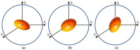
Figure 1.
Characteristic ellipsoids of the nonenpolarizing component of the extended form of a Mueller matrix M: (a) forward ellipsoid ; (b) canonical ellipsoid , of which the semiaxes (with ) are aligned with the Poincaré axes , respectively; and (c) reverse ellipsoid .
All three characteristic ellipsoids are centered (the center of the ellipsoid coincides with the origin of the Poincaré sphere) and have the same shape, with semiaxes . The symmetry axes of the canonical ellipsoid are aligned to the respective axes of the Poincaré sphere. Both forward and reverse ellipsoids, and , are rotated by the respective effects of and .
Degenerate cases occur when with (the characteristic ellipsoids become ellipses), with (straight segments), and (single point), which corresponds to the trivial limiting case of the zero Mueller matrix.
4.2. Enpolarizing Components
As for the components and , their associated coherency matrices and have the following respective sets of eigenvalues:
which are nonnegative because the conditions and are always satisfied by any Mueller matrix M [11].
Thus, can have either two or four parallel pure components (two when and four when ), and the same happens for depending on whether (two parallel pure components) or (four parallel pure components).
As occurs with component , the passivity of M implies the passivity of both and .
Moreover, both and are type-I singular Mueller matrices, which is evident when they are expressed as the following respective serial decompositions:
where and represent respective normal diattenuators defined based on vectors P and D [10,32,33,34], represents an arbitrary retarder (which plays no role in the definitive forms of and ), stands for the Kronecker product, and is the 3 × 3 identity matrix.
Since and are singular, their characteristic ellipsoids are given by single points [35]. In particular, as shown in Figure 2 and Figure 3, the canonical and reverse ellipsoids of , as well as the forward and canonical ellipsoids of , are single points located in the center of the Poincaré sphere, whereas the forward ellipsoid of and the reverse ellipsoid of are given by single points located within or on the surface of the Poincaré sphere depending on whether or , respectively.
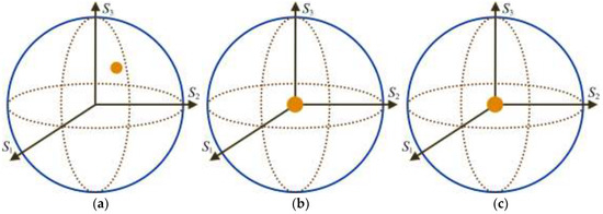
Figure 2.
The characteristic ellipsoids of the polarizing component of the homogeneous extended form of a Mueller matrix M are given by single points (the three semiaxes are zero-valued): (a) forward ellipsoid, , which lies on the surface of the Poincaré sphere if and only if ; (b) canonical ellipsoid ; and (c) reverse ellipsoid .
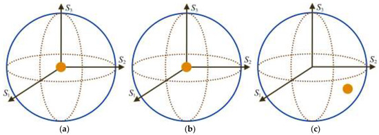
Figure 3.
The characteristic ellipsoids of the polarizing component of the homogeneous extended form of a Mueller matrix M are given by single points (the three semiaxes are zero-valued): (a) forward ellipsoid ; (b) canonical ellipsoid ; and (c) reverse ellipsoid, , which lies on the surface of the Poincaré sphere if and only if .
5. Extended Decomposition of a Mueller Matrix
As in Section 4, we consider here general Mueller matrices with nonzero polarizance and diattenuation . The cases where or will be dealt with in Section 6.
As an alternative to the homogeneous extended form of M, the MIC of the perfect depolarizer added to M can be taken as (instead of ), so that the extended form of M is defined as
Note that, since , the MIC of the perfect depolarizer, , is smaller than that of the perfect depolarizer in the homogeneous extended form, .
The extended decomposition of M is then defined as
Here, unlike the homogeneous extended decomposition, the polarizing and diattenuating components exhibit respective polarizance and diattenuation vectors, and , having necessarily maximal absolute values , and consequently the coherency matrices and have the following respective sets of eigenvalues:
so that .
In accordance with this property, both the forward ellipsoid of and the reverse ellipsoid of are given by single points that are located on the surface of the Poincaré sphere.
The structure of the components of the extended decomposition is even simpler than that of the homogeneous one. In particular, and can be interpreted by means of the following respective two-component parallel compositions:
where the nondepolarizing components of and correspond to respective perfect polarizers (i.e., media that fully polarize light entering either in the forward or reverse directions).
Note also that, as with the homogeneous extended decomposition, the passivity of the three components is ensured by the passivity of M itself.
The extended decomposition of the arrow form has the simple form
6. Extended Decompositions of Matrices Lacking Polarizance or Diattenuation
The extended decompositions introduced in Section 4 and Section 5 apply to Mueller matrices with nonzero polarizance and diattenuation ( and ). When or , the required ratio between the perfect depolarizer and the starting M for a well-defined extended form of M, without an excess of , changes with respect to the case where and . Appropriate particular forms of extended decompositions are analyzed below, which, together those dealt with in Section 4 and Section 5, provide a complete case analysis.
When and (nondiattenuating Mueller matrices, denoted as ), the extended decompositions of M take the following forms, where the denominator of the coefficients (polarimetric cross sections) equals the number of components (two):
Analogously, when and (nonpolarizing Mueller matrices, denoted as ),
The Mueller matrices , , of the components in the above equations have the forms defined in Equations (17) and (24).
In the case of a nonenpolarizing Mueller matrix , it directly has the form of the nonenpolarizing component and therefore its extended form coincides with itself (i.e., the corresponding coefficient for the added perfect depolarizer is zero).
7. Discussion
The extended representation of a given Mueller matrix M involves its convex sum with a perfect depolarizer , which does not exhibit any anisotropy (or polarimetric preference). Consequently, the anisotropies inherited by the extended representations and are precisely those of M. Furthermore, for any given M, both and are biunivocally related to M through simple expressions. In fact, the m, P, and D of are none other than those of M, whereas the structure of is given by m, , , P, and D (with and ).
Furthermore, the extended forms and in Equations (16) and (23) involving , of which the associated coherency matrix is , ensure that the respective coherency matrices and satisfy , which extends substantially the scope of parallel decompositions of the extended forms in comparison to those directly applicable to M, and makes it possible to obtain the extended decompositions considered in Section 4, Section 5 and Section 6.
It is remarkable that all Mueller matrices , , , , and of the constituents of the extended forms of M are type-I, and are therefore free from the intricate structure exhibited by type-II Mueller matrices [28,36].
Due to their simplicity, the extended forms and decompositions of any given Mueller matrix M can be straightforwardly interpreted regardless of its structural complexity. When the arrow form of M is considered, the analysis becomes even simpler because in that case, once the entrance and exit retarders have been decoupled from M, becomes diagonal [37].
An interesting limiting situation is that corresponding to pure Mueller matrices, of which the general structure adopts the form [38]
where and are equivalent (entrance and exit) linear retarders (each depending on two angular parameters), represents a horizontal linear retarder (depending on a single parameter), and is the normalized Mueller matrix of a normal [32,33,34] horizontal linear diattenuator which only depends on the polarizance-diattenuation D of (recall that pure Mueller matrices necessarily satisfy [39]).
Therefore, the extended components of the arrow form of are given by
Coming back to general Mueller matrices (depolarizing or not), observe that since the extended representation applies to any Mueller matrix without restriction, the following question may arise: given an arbitrary set of normalized matrices of the form , , and , is the 4 × 4 matrix retrieved as from in Equation (17) a (normalized) Mueller matrix? The answer is negative, as evidenced by taking, for instance, the following set of matrices:
for which does not satisfy the covariance conditions (i.e., it is not a Mueller matrix) because its associated coherency matrix has, at least, a negative eigenvalue.
8. Conclusions
The Mueller matrices obtained through certain parallel combinations of a given Mueller matrix M and a perfect depolarizer are always susceptible to be submitted to respective kinds of parallel decompositions named the homogeneous extended decomposition and the extended decomposition, the components of which have very simple structures which are directly inherited from the anisotropies exhibited by M.
The parallel composition of M and a perfect depolarizer, with appropriate convex coefficients, only affects the MIC (mean intensity coefficient) of the resulting composed matrix, but it is the key for M to be interpreted in terms of the properties of the components of the corresponding extended decompositions. In particular, two components can be straightforwardly determined from the polarizance and diattenuation vectors of M, respectively, whereas the third component depends exclusively on the 3 × 3 submatrix m of M, which encompasses the remaining polarimetric information. That is to say, once the information on polarizance and diattenuation has been decoupled and allocated to respective parallel components, the structure of the remaining nonenpolarizing component allows for the recovery of the complete polarimetric information (including the depolarization and retardance properties) held by M.
In summary, any Mueller matrix M (depolarizing or nondepolarizing) is susceptible to being represented, uniquely, through the extended representations and , and admits respective extended decompositions where the structural properties of M appear decoupled in a very simple manner and encoded into separate components.
Author Contributions
Conceptualization, I.S.J.; and J.J.G.; methodology, I.S.J.; and J.J.G.; writing—original draft preparation, I.S.J.; and J.J.G.; writing—review and editing, I.S.J.; and J.J.G. All authors have read and agreed to the published version of the manuscript.
Funding
This research received no external funding.
Informed Consent Statement
Not applicable.
Data Availability Statement
Not applicable.
Conflicts of Interest
The author declares no conflict of interest.
References
- Gil, J.J. Polarimetric characterization of light and media-Physical quantities involved in polarimetric phenomena. Eur. Phys. J. Appl. Phys. 2007, 40, 1–47. [Google Scholar] [CrossRef]
- Gil, J.J. Parallel decompositions of Mueller matrices and polarimetric subtraction. EPJ Web Conf. 2010, 5, 04002. [Google Scholar] [CrossRef]
- Gil, J.J.; San José, I. Arbitrary decomposition of a Mueller matrix. Opt. Lett. 2019, 44, 5715–5718. [Google Scholar] [CrossRef]
- Cloude, S.R. Group theory and polarization algebra. Optik 1986, 75, 26–36. [Google Scholar]
- Gil, J.J.; San José, I. Polarimetric subtraction of Mueller matrices. J. Opt. Soc. Am. A 2013, 30, 1078–1088. [Google Scholar] [CrossRef] [PubMed]
- Gil, J.J.; Ossikovski, R. Polarized Light and the Mueller Matrix Approach, 2nd Ed; CRC Press: Boca Raton, FL, USA, 2022. [Google Scholar]
- Gil, J.J. On optimal filtering of measured Mueller matrices. Appl. Opt. 2016, 55, 5449–5455. [Google Scholar] [CrossRef]
- Robson, B.A. The Theory of Polarization Phenomena; Clarendon Press: Oxford, UK, 1975. [Google Scholar]
- Xing, Z.-F. On the deterministic and non-deterministic Mueller matrix. J. Mod. Opt. 1992, 39, 461–484. [Google Scholar] [CrossRef]
- Lu, S.-Y.; Chipman, R.A. Interpretation of Mueller matrices based on polar decomposition. J. Opt. Soc. Am. A 1996, 13, 1106–1113. [Google Scholar] [CrossRef]
- Gil, J.J.; Bernabéu, E. Depolarization and polarization indices of an optical system. Opt. Acta 1986, 33, 185–189. [Google Scholar] [CrossRef]
- Gil, J.J. Components of purity of a Mueller matrix. J. Opt. Soc. Am. A 2011, 28, 1578–1585. [Google Scholar] [CrossRef]
- Gil, J.J. Thermodynamic reversibility in polarimetry. Photonics 2022, 9, 650. [Google Scholar] [CrossRef]
- Gil, J.J. Structure of polarimetric purity of a Mueller matrix and sources of depolarization. Opt. Commun. 2016, 368, 165–173. [Google Scholar] [CrossRef]
- Gil, J.J.; San José, I.; Ossikovski, R. Serial–Parallel decompositions of Mueller matrices. J. Opt. Soc. Am. A 2013, 30, 32–50. [Google Scholar] [CrossRef]
- Gil, J.J. Characteristic properties of Mueller matrices. J. Opt. Soc. Am. A 2000, 17, 328–334. [Google Scholar] [CrossRef] [PubMed]
- San José, I.; Gil, J.J. Characterization of passivity in Mueller matrices. J. Opt. Soc. Am. A 2020, 37, 199–208. [Google Scholar] [CrossRef]
- Sekera, Z. Scattering Matrices and Reciprocity Relationships for Various Representations of the State of Polarization. J. Opt. Soc. Am. 1966, 56, 1732–1740. [Google Scholar] [CrossRef]
- Schönhofer, A.; Kuball, H.-G. Symmetry properties of the Mueller matrix. Chem. Phys. 1987, 115, 159–167. [Google Scholar] [CrossRef]
- Ossikovski, R.; De Martino, A.; Guyot, S. Forward and reverse product decompositions of depolarizing Mueller matrices. Opt. Lett. 2007, 32, 689–691. [Google Scholar] [CrossRef]
- Van der Mee, C.V.M. An eigenvalue criterion for matrices transforming Stokes parameters. J. Math. Phys. 1993, 34, 5072–5088. [Google Scholar] [CrossRef]
- Sridhar, R.; Simon, R. Normal form for Mueller matrices in polarization optics. J. Mod. Opt. 1994, 41, 1903–1915. [Google Scholar] [CrossRef]
- Bolshakov, Y.; van der Mee, C.V.M.; Ran, A.C.M.; Reichstein, B.; Rodman, L. Polar decompositions in finite dimensional indefinite scalar product spaces: Special cases and applications. In Operator Theory: Advances and Applications; Gohberg, I., Ed.; Birkhäuser: Basel, Switzerland, 1996; Volume 87, pp. 61–94. [Google Scholar]
- Bolshakov, Y.; van der Mee, C.V.M.; Ran, A.C.M.; Reichstein, B.; Rodman, L. Errata for: Polar decompositions in finite dimensional indefinite scalar product spaces: Special cases and applications. Integral Equ. Oper. Theory 1997, 27, 497–501. [Google Scholar] [CrossRef]
- Gopala Rao, A.V.; Mallesh, K.S.; Sudha. On the algebraic characterization of a Mueller matrix in polarization optics. I. Identifying a Mueller matrix from its N matrix. J. Mod. Opt. 1998, 45, 955–987. [Google Scholar]
- Gopala Rao, A.V.; Mallesh, K.S.; Sudha. On the algebraic characterization of a Mueller matrix in polarization optics. II. Necessary and sufficient conditions for Jones derived Mueller matrices. J. Mod. Opt. 1998, 45, 989–999. [Google Scholar]
- Ossikovski, R. Analysis of depolarizing Mueller matrices through a symmetric decomposition. J. Opt. Soc. Am. A 2009, 26, 1109–1118. [Google Scholar] [CrossRef] [PubMed]
- Ossikovski, R. Canonical forms of depolarizing Mueller matrices. J. Opt. Soc. Am. A 2010, 27, 123–130. [Google Scholar] [CrossRef] [PubMed]
- Ossikovski, R.; Gil, J.J.; San José, I. Poincaré sphere mapping by Mueller matrices. J. Opt. Soc. Am. A 2013, 30, 2291–2305. [Google Scholar] [CrossRef]
- Gil, J.J. Transmittance constraints in serial decompositions of Mueller matrices. The arrow form of a Mueller matrix. J. Opt. Soc. Am. A 2013, 30, 701–707. [Google Scholar] [CrossRef]
- Gil, J.J. Invariant quantities of a Mueller matrix under rotation and retarder transformations. J. Opt. Soc. Am. A 2016, 33, 52–58. [Google Scholar] [CrossRef]
- Lu, S.-Y.; Chipman, R.A. Homogeneous and inhomogeneous Jones matrices. J. Opt. Soc. Am. A 1994, 11, 766–773. [Google Scholar] [CrossRef]
- Tudor, T.; Gheondea, A. Pauli algebraic forms of normal and non-normal operators. J. Opt. Soc. Am. A 2007, 24, 204–210. [Google Scholar] [CrossRef]
- Tudor, T. Interaction of light with the polarization devices: A vectorial Pauli algebraic approach. J. Phys. A-Math. Theor 2008, 41, 41530. [Google Scholar] [CrossRef]
- Gil, J.J.; Ossikovski, R.; San José, I. Singular Mueller matrices. J. Opt. Soc. Am. A 2016, 33, 600–609. [Google Scholar] [CrossRef]
- San José, I.; Gil, J.J.; Ossikovski, R. Algorithm for the numerical calculation of the serial components of the normal form of depolarizing Mueller matrices. Appl. Opt. 2020, 59, 2291–2297. [Google Scholar] [CrossRef] [PubMed]
- Gil, J.J.; San José, I. Universal Synthesizer of Mueller Matrices Based on the Symmetry Properties of the Enpolarizing Ellipsoid. Symmetry 2021, 13, 983. [Google Scholar] [CrossRef]
- Gil, J.J.; San José, I. Invariant quantities of a nondepolarizing Mueller matrix. J. Opt. Soc. Am. A 2016, 133, 1307–1312. [Google Scholar] [CrossRef] [PubMed]
- Gil, J.J. Determination of Polarization Parameters in Matricial Representation. Theoretical Contribution and Development of an Automatic Measurement Device. Ph.D. Dissertation, University of Zaragoza, Zaragoza, Spain, 1983. Available online: http://zaguan.unizar.es/record/10680/files/TESIS-2013-057.pdf (accessed on 5 December 2022).
Disclaimer/Publisher’s Note: The statements, opinions and data contained in all publications are solely those of the individual author(s) and contributor(s) and not of MDPI and/or the editor(s). MDPI and/or the editor(s) disclaim responsibility for any injury to people or property resulting from any ideas, methods, instructions or products referred to in the content. |
© 2023 by the authors. Licensee MDPI, Basel, Switzerland. This article is an open access article distributed under the terms and conditions of the Creative Commons Attribution (CC BY) license (https://creativecommons.org/licenses/by/4.0/).