Distributed PD Average Consensus of Lipschitz Nonlinear MASs in the Presence of Mixed Delays

Abstract

In this work, the distributed average consensus for dynamical networks with Lipschitz nonlinear dynamics is studied, where the network communication switches quickly among a set of directed and balanced switching graphs. Differing from existing research concerning uniform constant delay or time-varying delays, this study focuses on consensus problems with mixed delays, equipped with one class of delays embedded within the nonlinear dynamics and another class of delays present in the control input. In order to solve these problems, a proportional and derivative control strategy with time delays is proposed. In this way, by using Lyapunov theory, the stability is analytically established and the conditions required for solving the consensus problems are rigorously derived over switching digraphs. Finally, the effectiveness of the designed algorithm is tested using the MATLAB R2021a platform.

1. Introduction

Multi-agent systems (MASs), as a class of complex networks, have garnered considerable attention across a variety of fields, encompassing urban transportation [1], smart grids [2], communication optimization [3], the national defense industry [4], and others. Over recent decades, numerous intriguing and valuable insights into the study of MASs have been presented [5,6,7,8,9,10,11,12]. Notably, consensus represents a pivotal collective behavior within MASs, and it stands out as the predominant research focus in this area given its extensive applications in large-scale formation control [13,14] and flocking behavior [15]. Average consensus [16], a distinct type of consensus, pertains to the task of computing the average of certain quantities, differing from seeking a common value. Recently, a substantial number of reports have emerged which broaden the scope of average consensus results to encompass more generalized dynamics and communication environments [17,18,19,20,21].

However, it is noteworthy that physical systems frequently possess delay characteristics. The need to address the consensus challenge in MASs subject to time delays has led to the emergence of many intriguing findings. In particular, Sun et al. [22] discussed the mean square average consensus for first-order integrators with a communication constant time delay (CTD) obtained by means of the stopping time truncation approach. Over a balanced digraph, Liu et al. [23] developed the average consensus filter for first-order integrators with heterogeneous disturbances considering a communication CTD. For arbitrarily large CTDs, Aragues et al. [24] introduced delay compensation techniques to address the average consensus for discrete-time MASs over a strongly connected graph. Furthermore, in [25], the consensus for nonlinear MASs with unknown-state CTDs was studied, and was found to depend on a neural network control law over an undirected graph. Based on [25], Ma et al. [26] dealt with the robust consensus problem with unknown-state CTDs and external noises over an undirected graph. Soon after, Wen et al. [27] investigated the consensus tracking problem in the existence of unknown-state CTDs and exogenous disturbances by proposing an adaptive control algorithm.

It should be pointed out that the studies mentioned above only consider the problems with CTDs; however, delay is usually time-varying in practical systems. For example, Wang et al. [28] adopted a proportional and derivative (PD) control law to cope with average consensus problems subject to a communication time-varying delay (TVD) over switching digraphs. In [29], the reciprocally convex approach was employed to tackle the local consensus problem with communication TVDs under a strongly connected digraph. Inspired by the work [30] subject to CTDs, Ma et al. [31] developed proportional and PD feedback laws to analyze the robust consensus with communication TVDs over both undirected and directed graphs. In the context of a cooperative-antagonistic framework, Caiazzo et al. [32] solved the average consensus with multiple unknown TVDs over a signed graph. Moreover, for a high-order integrator network with nonlinear dynamics, the consensus problem was addressed over a undirected graph in the work of [33] subject to state TVDs by using an edge-based self-triggering impulsive protocol, and consensus conditions were obtained in [34] under switching graphs by proposing a PD protocol in the presence of communication TVDs. In addition, other achievements about consensus problems with different TVDs can be found in [35,36,37,38,39,40,41,42].

From the discussion presented above, it becomes evident that state and communication delays within the system are crucial elements influencing the consensus results. There exists considerable potential for enhancing current research endeavors through the application of novel analysis techniques. Therefore, we investigate the average consensus for nonlinear MASs with mixed TVDs over switching digraphs. Thus, the distinct contributions of this study are highlighted as follows: First, to achieve superior performance index, a distributed PD control law with TVDs is utilized to tackle the average consensus of MASs with Lipschitz nonlinearity. Second, this paper is concerned with the average consensus problems over a balanced graph rather than assuming the communication graph is undirected. Third, we take into account both the state and communication TVDs, as well as inner nonlinearities. Importantly, state TVDs and communication delays are not identical. Fourth, the sufficient conditions of combined linear matrix inequalities (LMIs) can be obtained based on the formulation of appropriate Lyapunov–Krasovskii functionals (LKFs) containing triple integral terms.

The remaining parts are structured as follows: the preliminaries and problem formulation are presented in Section 2. Section 3 shows the average consensus design condition and main results. In Section 4, a simulation example is provided. Finally, Section 5 concludes this paper.

2. Preliminaries and Problem Formulation

2.1. Preliminaries and Notations

The communication graph is described by $\mathcal{G}=\left.\left\{\mathcal{V},\mathcal{E},\mathcal{A}\right.\right\}$, which consists of N nodes $\mathcal{V}=\{1,\dots ,N\}$, the edges $\mathcal{E}=\left.\left\{(i,j):i,j\in \mathcal{V}\right.\right\}$, and an adjacency matrix $\mathcal{A}=\left[a_{ij}\right]\in R^{N\times N}$, with $a_{ij}=1$ if $(i,j)\in \mathcal{E}$ and $a_{ij}=0$ otherwise. $\mathcal{G}$ is a balanced graph when ${\sum }_{j=1}^N{a}_{ij}={\sum }_{j=1}^N{a}_{ji}$ for $i\in \mathcal{V}$ [43]. The Laplacian matrix is denoted as $L=diag\left\{{\sum }_{j=1}^N{a}_{ij}\right\}-\mathcal{A}$. Moreover, let ∗ represent the symmetric term, $\mathrm{col}(x_1,\dots ,x_n)=[x_1^T,\dots ,x_n^T{]}^T$ and $1_n={[1,\dots ,1]}^T$.

2.2. Problem Formulation

The dynamics of the ith agent is denoted by

$$\begin{array}{c}\hfill {\dot{x}}_i\left(t\right)=g\left(x_i(t-d\left(t\right))\right)+u_i\left(t\right),\end{array}$$

(1)

where $x_i\left(t\right)\in R^n$ and $u_i\left(t\right)\in R^n$ represent the state variable and the control input of agent i. For ease of understanding, the dimension $n=1$ is used through the paper. $g\left(x_i(t-d\left(t\right))\right)$ denotes the inner nonlinear function, and $d\left(t\right)$ represents the TVD. Note that $0\le d\left(t\right)\le k,{\widehat{\mu }}_1\le \dot{d}\left(t\right)\le {\mu }_1,0<\left|{\widehat{\mu }}_1\right|<1,0<\left|{\mu }_1\right|<1$.

Definition 1

([44]). The average consensus can be achieved if the condition $\underset{t\to \infty }{lim}{x}_i\left(t\right)={\displaystyle \frac{1}{N}}{\displaystyle \sum _{j=1}^N}{x}_j\left(0\right)$ holds for $i,j\in \mathcal{V}$.

The switching interaction graph of N agents in (1) is modeled by a switched connected graph ${\mathcal{G}}_{\mathrm{\sigma }}$, and $\mathrm{\sigma }:\left[0,\infty \right)\to \mathcal{P}$ indicates a graph in $\mathcal{P}\stackrel{\Delta }{=}\{1,2,\dots ,M\}$ at time t, while $\{{\mathcal{G}}_{\mathrm{\sigma }}:\mathrm{\sigma }\in \mathcal{P}\}$ denotes a fixed graph in set $\left\{{\cup }_{t\ge 0}\mathcal{G}\right\}$.

Assumption A1.

${\mathcal{G}}_{\mathrm{\sigma }}$ is directed, connected, and balanced for each $\mathrm{\sigma }\in \mathcal{P}$.

Assumption A2.

If a nonlinear function $g(.)$ satisfies the Lipschitz condition, there exists a nonnegative constant q such that

$$\begin{array}{c}\hfill ∥g(t,x(t\left)\right)-g(t,y(t\left)\right)∥\le {\displaystyle \frac{q}{2}}∥x\left(t\right)-y\left(t\right)∥,\forall x\left(t\right),y\left(t\right)\in R^n.\end{array}$$

Lemma 1

([45]). If Assumption 1 holds, the Laplacian matrix $L\in R^{N\times N}$ satisfies $1_N^{T}L=0$ and $L{1}_N=0$.

Lemma 2

([46]). For the matrix $\mathrm{{\rm Y}}={\mathrm{{\rm Y}}}^T>0$ and scalar $\upsilon >0$, the subsequent condition holds that

$$\begin{array}{c}\hfill {\int }_{-\upsilon }^0{\int }_{t+\theta }^t{\varpi }^T\left(s\right)\mathrm{{\rm Y}}\varpi \left(s\right)dsd\theta \ge {\displaystyle \frac{1}{{\upsilon }^2}}{\left({\int }_{-\upsilon }^0{\int }_{t+\theta }^t\varpi \left(s\right)dsd\theta \right)}^T\mathrm{{\rm Y}}\mathrm{{\rm Y}}\left({\int }_{-\upsilon }^0{\int }_{t+\theta }^t\varpi \left(s\right)dsd\theta \right).\end{array}$$

3. Average Consensus Design Condition

A PD control law considering delay $\tau \left(t\right)$ is proposed as follows:

$$\begin{array}{cc}\hfill u_i\left(t\right)=& -\beta \sum _{j\in {\mathcal{N}}_i}{a}_{ij}\left(t\right)[x_i(t-\tau \left(t\right))-x_j(t-\tau \left(t\right))]\hfill \\ \hfill & -\alpha \sum _{j\in {\mathcal{N}}_i}{a}_{ij}\left(t\right)[{\dot{x}}_i(t-\tau \left(t\right))-{\dot{x}}_j(t-\tau \left(t\right))],\hfill \end{array}$$

(2)

where $\beta$ and $\alpha$ are positive parameters and $\tau \left(t\right)$ is the communication delay which satisfies $0\le \tau \left(t\right)\le h,{\widehat{\mu }}_2\le \dot{\tau }\left(t\right)\le {\mu }_2,0<\left|{\widehat{\mu }}_2\right|<1,0<\left|{\mu }_2\right|<1.$

Remark 1.

Different from the proportional control protocols [11,12,22,29,44], the two parameters β and α are designed in (2), where greater flexibility in the PD control protocol is provided. Furthermore, the convergence rate in (2) is improved in comparison with those proportional protocols. In addition, the PD scheme boasts superior advantages, as shown in [28,30,31,34].

Substituting (2) into (1) yields

$$\begin{array}{cc}\hfill {\dot{x}}_i\left(t\right)=& -\beta \sum _{j\in {\mathcal{N}}_i}{a}_{ij}\left(t\right)[x_i(t-\tau \left(t\right))-x_j(t-\tau \left(t\right))]\hfill \\ \hfill & -\alpha \sum _{j\in {\mathcal{N}}_i}{a}_{ij}\left(t\right)[{\dot{x}}_i(t-\tau \left(t\right))-{\dot{x}}_j(t-\tau \left(t\right))]+g\left(x_i(t-d\left(t\right))\right).\hfill \end{array}$$

(3)

Let $x\left(t\right)=\mathrm{col}(x_1\left(t\right),\dots ,x_N\left(t\right))$, $x(t-\tau \left(t\right))=\mathrm{col}(x_1(t-\tau \left(t\right)),\dots ,x_N(t-\tau \left(t\right)))$ and $g\left(x(t-d\left(t\right))\right)=\mathrm{col}(g\left(x_1(t-d\left(t\right))\right),\dots ,g\left(x_N(t-d\left(t\right))\right))$. Then, it follows from (3) that

$$\begin{array}{c}\hfill \dot{x}\left(t\right)=-\beta L_{\mathrm{\sigma }}x(t-\tau \left(t\right))-\alpha L_{\mathrm{\sigma }}\dot{x}(t-\tau \left(t\right))+g\left(x(t-d\left(t\right))\right).\end{array}$$

(4)

Furthermore, let $\stackrel{-}{x}\left(t\right)=\left({\displaystyle \raisebox{1ex}{$1$}\!\left/ \!\raisebox{-1ex}{$N$}\right.}\right){\sum }_{i=1}^N{x}_i\left(t\right)$, $\stackrel{-}{g}\left(x(t-d\left(t\right))\right)=\left({\displaystyle \raisebox{1ex}{$1$}\!\left/ \!\raisebox{-1ex}{$N$}\right.}\right){\sum }_{i=1}^{N}g\left(x_i(t-d\left(t\right))\right)$ and $z\left(t\right)=x\left(t\right)-1_N\otimes \stackrel{-}{x}\left(t\right)$. Thus, Equation (4) can easily be transformed into

$$\begin{array}{c}\hfill \dot{z}\left(t\right)=-\beta L_{\mathrm{\sigma }}z(t-\tau \left(t\right))-\alpha L_{\mathrm{\sigma }}\dot{z}(t-\tau \left(t\right))+G\left(x(t-d\left(t\right))\right),\end{array}$$

(5)

where $G\left(x(t-d\left(t\right))\right)=g\left(x(t-d\left(t\right))\right)-1_N\otimes \stackrel{-}{g}\left(x(t-d\left(t\right))\right)$.

According to Assumption 2, this yields

$$\begin{array}{cc}\hfill ∥G\left(x\right(t-d\left(t\right)\left)\right)∥\le & ∥g\left(x(t-d\left(t\right))\right)-1_N\otimes g\left(\stackrel{-}{x}(t-d\left(t\right))\right)∥\hfill \\ \hfill & +∥1_N\otimes g\left(\stackrel{-}{x}(t-d\left(t\right))\right)-1_N\otimes \stackrel{-}{g}\left(x(t-d\left(t\right))\right)∥\hfill \\ \hfill \le & \left({\displaystyle \raisebox{1ex}{$q$}\!\left/ \!\raisebox{-1ex}{$2$}\right.}\right)∥z(t-d(t\left)\right)∥+\left({\displaystyle \raisebox{1ex}{$1$}\!\left/ \!\raisebox{-1ex}{$N$}\right.}\right){\sum }_{i=1}^N∥g\left(x_i(t-d\left(t\right))\right)-g\left(\stackrel{-}{x}(t-d\left(t\right))\right)∥\hfill \\ \hfill \le & q∥z(t-d(t\left)\right)∥.\hfill \end{array}$$

(6)

Theorem 1.

Suppose that ${\mathcal{G}}_{\mathrm{\sigma }}$ ($\mathrm{\sigma }\in \mathcal{P}$) is directed, connected, and balanced. For the given parameters ${\mu }_i>0(i=1,2)$, $\alpha >0$, $\beta >0$, $q>0$, $h>0$, $k>0$ and ${\widehat{\mu }}_1$, the average consensus of nonlinear MASs (1) with mixed TVDs is realized by a PD protocol (2) if there exist the matrices $R>0$, $P_i>0$, $S_i>0$, $Y_i>0$, $Q_i>0$, $W_i>0$, $T_i>0$, $Q_{ii}>0$, $i=1,2$, such that $P_1+(k-d\left(t\right))P_2>0$ and the following conditions hold:

$$\begin{array}{cc}\hfill {\tilde{\mathrm{\Psi }}}_{\mathrm{\sigma }}=& {\left[\begin{array}{ccc}{\tilde{\mathrm{\Psi }}}_{1\mathrm{\sigma }}& {\tilde{\mathrm{\Psi }}}_{2\mathrm{\sigma }}& {\tilde{\mathrm{\Psi }}}_{3\mathrm{\sigma }}\\ \ast & {\mathrm{\Psi }}_{4\mathrm{\sigma }}& {\mathrm{\Psi }}_{5\mathrm{\sigma }}\\ \ast & \ast & {\mathrm{\Psi }}_{6\mathrm{\sigma }}\end{array}\right]}_{d\left(t\right)=0}<0,\hfill \end{array}$$

(7a)

$$\begin{array}{cc}\hfill {\widehat{\mathrm{\Psi }}}_{\mathrm{\sigma }}=& {\left[\begin{array}{ccc}{\widehat{\mathrm{\Psi }}}_{1\mathrm{\sigma }}& {\widehat{\mathrm{\Psi }}}_{2\mathrm{\sigma }}& {\widehat{\mathrm{\Psi }}}_{3\mathrm{\sigma }}\\ \ast & {\mathrm{\Psi }}_{4\mathrm{\sigma }}& {\mathrm{\Psi }}_{5\mathrm{\sigma }}\\ \ast & \ast & {\mathrm{\Psi }}_{6\mathrm{\sigma }}\end{array}\right]}_{d\left(t\right)=k}<0,\hfill \end{array}$$

(7b)

$$\begin{array}{cc}\hfill {\tilde{Q}}_1=& \left[\begin{array}{cc}{Q}_1& Y_1\\ \ast & S_1\end{array}\right]>0,\hfill \end{array}$$

(7c)

$$\begin{array}{cc}\hfill {\tilde{Q}}_2=& \left[\begin{array}{cc}{Q}_2& Y_2\\ \ast & S_2\end{array}\right]>0,\hfill \end{array}$$

(7d)

where

$$\begin{array}{c}\hfill \begin{array}{c}{\tilde{\mathrm{\Psi }}}_{1\mathrm{\sigma }}=\left[\begin{array}{ccc}{\tilde{\theta }}_{11\mathrm{\sigma }}& 0& W_2\\ \ast & {\tilde{\theta }}_{22\mathrm{\sigma }}& 0\\ \ast & \ast & -Q_{11}-W_2\end{array}\right],{\tilde{\mathrm{\Psi }}}_{2\mathrm{\sigma }}=\left[\begin{array}{ccc}{\tilde{\theta }}_{14\mathrm{\sigma }}& W_1& 0\\ 0& 0& 0\\ 0& 0& 0\end{array}\right],\hfill \end{array}\end{array}$$

$$\begin{array}{c}\hfill \begin{array}{c}{\tilde{\mathrm{\Psi }}}_{3\mathrm{\sigma }}=\left[\begin{array}{ccc}{\tilde{\theta }}_{17\mathrm{\sigma }}& hR& 0\\ 0& 0& 0\\ 0& 0& 0\end{array}\right],{\mathrm{\Psi }}_{4\mathrm{\sigma }}=\left[\begin{array}{ccc}{\theta }_{44\mathrm{\sigma }}& 0& 0\\ \ast & -Q_1-W_1& -Y_1\\ \ast & \ast & -S_1\end{array}\right],\hfill \\ {\mathrm{\Psi }}_{6\mathrm{\sigma }}=\left[\begin{array}{ccc}{\theta }_{77\mathrm{\sigma }}& 0& 0\\ \ast & -R& 0\\ \ast & \ast & -{\displaystyle \frac{1}{h}}{T}_2\end{array}\right],{\widehat{\mathrm{\Psi }}}_{1\mathrm{\sigma }}=\left[\begin{array}{ccc}{\widehat{\theta }}_{11\mathrm{\sigma }}& 0& W_2\\ \ast & {\widehat{\theta }}_{22\mathrm{\sigma }}& 0\\ \ast & \ast & -Q_{11}-W_2\end{array}\right],\hfill \\ {\widehat{\mathrm{\Psi }}}_{2\mathrm{\sigma }}=\left[\begin{array}{ccc}{\widehat{\theta }}_{14\mathrm{\sigma }}& W_1& 0\\ 0& 0& 0\\ 0& 0& 0\end{array}\right],{\mathrm{\Psi }}_{5\mathrm{\sigma }}=\left[\begin{array}{ccc}{\theta }_{47\mathrm{\sigma }}& 0& 0\\ 0& 0& 0\\ 0& 0& 0\end{array}\right],{\widehat{\mathrm{\Psi }}}_{3\mathrm{\sigma }}=\left[\begin{array}{ccc}{\widehat{\theta }}_{17\mathrm{\sigma }}& hR& 0\\ 0& 0& 0\\ 0& 0& 0\end{array}\right],\hfill \end{array}\end{array}$$

with

$$\begin{array}{c}\hfill \begin{array}{c}\Theta =S_1+S_2+T_1+h^2{W}_1+k^2{W}_2+{\displaystyle \frac{1}{4}}{h}^{4}R;\hfill \\ {\tilde{\theta }}_{11\mathrm{\sigma }}={\widehat{\theta }}_{11\mathrm{\sigma }}+k{P}_2,{\tilde{\theta }}_{22\mathrm{\sigma }}={\widehat{\theta }}_{22\mathrm{\sigma }}+q^2{P}_2;\hfill \\ {\widehat{\theta }}_{11\mathrm{\sigma }}=P_1-{\widehat{\mu }}_1{P}_2+Q_1+Q_2+Y_1+Y_2+Q_{11}+Q_{22}+h{T}_2-h^{2}R-W_1-W_2;\hfill \\ {\widehat{\theta }}_{22\mathrm{\sigma }}=(1+\alpha +\beta )q^2\Theta +q^2(P_1+Y_1+Y_2)-(1-{\mu }_1)Q_{22};\hfill \\ {\tilde{\theta }}_{14\mathrm{\sigma }}={\widehat{\theta }}_{14\mathrm{\sigma }}-k\beta P_2{L}_{\mathrm{\sigma }},{\tilde{\theta }}_{17\mathrm{\sigma }}={\widehat{\theta }}_{17\mathrm{\sigma }}-k\alpha P_2{L}_{\mathrm{\sigma }};\hfill \\ {\widehat{\theta }}_{14\mathrm{\sigma }}=-\beta (P_1+Y_1)L_{\mathrm{\sigma }},{\theta }_{47\mathrm{\sigma }}=\beta \alpha L_{\mathrm{\sigma }}^T\Theta L_{\mathrm{\sigma }}-(1-{\mu }_2)Y_2;\hfill \\ {\widehat{\theta }}_{17\mathrm{\sigma }}=-\alpha (P_1+Y_1+Y)L_{\mathrm{\sigma }},{\theta }_{44\mathrm{\sigma }}=(\beta +{\beta }^2)L_{\mathrm{\sigma }}^T\Theta L_{\mathrm{\sigma }}-(1-{\mu }_2)Q_2;\hfill \\ {\theta }_{77\mathrm{\sigma }}=(\alpha +{\alpha }^2)L_{\mathrm{\sigma }}^T\Theta L_{\mathrm{\sigma }}-(1-{\mu }_2)(S_2+T_1).\hfill \end{array}\end{array}$$

Proof. 

Construct the LKF candidate for MASs (1) as

$$\begin{array}{c}\hfill V\left(t\right)=\sum _{m=1}^6{V}_m\left(t\right),\end{array}$$

(8)

where

$$\begin{array}{cc}\hfill V_1\left(t\right)& =z^T\left(t\right)P_{1}z\left(t\right)+z^T\left(t\right)(k-d\left(t\right))P_{2}z\left(t\right);\hfill \\ \hfill V_2\left(t\right)& ={\int }_{t-h}^t{\eta }^T\left(s\right){\tilde{Q}}_1\eta \left(s\right)ds+{\int }_{t-k}^t{z}^T\left(s\right)Q_{11}z\left(s\right)ds;\hfill \\ \hfill V_3\left(t\right)& =h{\int }_{-h}^0{\int }_{t+\theta }^t{\dot{z}}^T\left(s\right)W_1\dot{z}\left(s\right)dsd\theta +k{\int }_{-k}^0{\int }_{t+\theta }^t{\dot{z}}^T\left(s\right)W_2\dot{z}\left(s\right)dsd\theta ;\hfill \\ \hfill V_4\left(t\right)& ={\displaystyle \frac{h^2}{2}}{\int }_{-h}^0{\int }_{\theta }^0{\int }_{t+\lambda }^t{\dot{z}}^T\left(s\right)R\dot{z}\left(s\right)dsd\lambda d\theta ;\hfill \\ \hfill V_5\left(t\right)& ={\int }_{t-\tau \left(t\right)}^t{\dot{z}}^T\left(s\right)T_1\dot{z}\left(s\right)ds+{\int }_{-\tau \left(t\right)}^0{\int }_{t+\theta }^t{z}^T\left(s\right)T_{2}z\left(s\right)dsd\theta ;\hfill \\ \hfill V_6\left(t\right)& ={\int }_{t-\tau \left(t\right)}^t{\eta }^T\left(s\right){\tilde{Q}}_2\eta \left(s\right)ds+{\int }_{t-d\left(t\right)}^t{z}^T\left(s\right)Q_{22}z\left(s\right)ds;\hfill \\ \hfill \eta \left(t\right)& =\left[\begin{array}{c}z\left(t\right)\\ \dot{z}\left(t\right)\end{array}\right],{\tilde{Q}}_1=\left[\begin{array}{cc}{Q}_1& Y_1\\ \ast & S_1\end{array}\right],{\tilde{Q}}_2=\left[\begin{array}{cc}{Q}_2& Y_2\\ \ast & S_2\end{array}\right].\hfill \end{array}$$

Then, calculating the derivatives of $V\left(t\right)$ yields

$$\begin{array}{cc}\hfill {\dot{V}}_1\left(t\right)=& {\dot{z}}^T\left(t\right)P_{1}z\left(t\right)+z^T\left(t\right)P_1\dot{z}\left(t\right)+(k-d\left(t\right)){\dot{z}}^T\left(t\right)P_{2}z\left(t\right)\hfill \\ \hfill & +(k-d\left(t\right))z^T\left(t\right)P_2\dot{z}\left(t\right)-\dot{d}\left(t\right)z^T\left(t\right)P_{2}z\left(t\right),\hfill \end{array}$$

(9)

and it has

$$\begin{array}{cc}\hfill G^T\left(x(t-d\left(t\right))\right)P_1& z\left(t\right)+z^T\left(t\right)P_{1}G\left(x(t-d\left(t\right))\right)\hfill \\ \hfill & \le G^T\left(x(t-d\left(t\right))\right)P_{1}G\left(x(t-d\left(t\right))\right)+z^T\left(t\right)P_{1}z\left(t\right)\hfill \\ \hfill & \le q^2{z}^T(t-d\left(t\right))P_{1}z(t-d\left(t\right))+z^T\left(t\right)P_{1}z\left(t\right).\hfill \end{array}$$

Similarly, it achieves

$$\begin{array}{cc}\hfill G^T\left(x(t-d\left(t\right))\right)P_2& z\left(t\right)+z^T\left(t\right)P_{2}G\left(x(t-d\left(t\right))\right)\hfill \\ \hfill & \le q^2{z}^T(t-d\left(t\right))P_{2}z(t-d\left(t\right))+z^T\left(t\right)P_{2}z\left(t\right).\hfill \end{array}$$

We have

$$\begin{array}{cc}\hfill {\dot{V}}_2\left(t\right)& ={\left[\begin{array}{c}z\left(t\right)\\ \dot{z}\left(t\right)\end{array}\right]}^T\left[\begin{array}{cc}{Q}_1& Y_1\\ \ast & S_1\end{array}\right]\left[\begin{array}{c}z\left(t\right)\\ \dot{z}\left(t\right)\end{array}\right]\hfill \\ \hfill & -{\left[\begin{array}{c}z(t-h)\\ \dot{z}(t-h)\end{array}\right]}^T\left[\begin{array}{cc}{Q}_1& Y_1\\ \ast & S_1\end{array}\right]\left[\begin{array}{c}z(t-h)\\ \dot{z}(t-h)\end{array}\right]\hfill \\ \hfill & +z^T\left(t\right)Q_{11}z\left(t\right)-z^T(t-k)Q_{11}z(t-k).\hfill \end{array}$$

(10)

This yields

$$\begin{array}{cc}\hfill \dot{z}\left(t\right)S_1\dot{z}\left(t\right)=& {\beta }^2{z}^T(t-\tau \left(t\right))L_{\mathrm{\sigma }}^T{S}_1{L}_{\mathrm{\sigma }}z(t-\tau \left(t\right))+\beta \alpha z^T(t-\tau \left(t\right))L_{\mathrm{\sigma }}^T{S}_1{L}_{\mathrm{\sigma }}\dot{z}(t-\tau \left(t\right))\hfill \\ \hfill & +\beta \alpha {\dot{z}}^T(t-\tau \left(t\right))L_{\mathrm{\sigma }}^T{S}_1{L}_{\mathrm{\sigma }}z(t-\tau \left(t\right))+{\alpha }^2{\dot{z}}^T(t-\tau \left(t\right))L_{\mathrm{\sigma }}^T{S}_1{L}_{\mathrm{\sigma }}{\dot{z}}^T(t-\tau \left(t\right))\hfill \\ \hfill & -2\beta z^T(t-\tau \left(t\right))L_{\mathrm{\sigma }}^T{S}_1{L}_{\mathrm{\sigma }}G\left(x(t-d\left(t\right))\right)-2\alpha {\dot{z}}^T(t-\tau \left(t\right))L_{\mathrm{\sigma }}^T{S}_1{L}_{\mathrm{\sigma }}G\left(x(t-d\left(t\right))\right)\hfill \\ \hfill & +G^T\left(x(t-d\left(t\right))\right)S_{1}G\left(x(t-d\left(t\right))\right),\hfill \end{array}$$

and we can easily get

$$\begin{array}{c}\hfill \begin{array}{c}-2\beta z^T(t-\tau \left(t\right))L_{\mathrm{\sigma }}^T{S}_1{L}_{\mathrm{\sigma }}G\left(x(t-d\left(t\right))\right)\hfill \\ \le \beta z^T(t-\tau \left(t\right))L_{\mathrm{\sigma }}^T{S}_1{L}_{\mathrm{\sigma }}z(t-\tau \left(t\right))+\beta q^2{z}^T(t-d\left(t\right))S_{1}z(t-d\left(t\right)),\hfill \\ -2\alpha {\dot{z}}^T(t-\tau \left(t\right))L_{\mathrm{\sigma }}^T{S}_1{L}_{\mathrm{\sigma }}G\left(x(t-d\left(t\right))\right)\hfill \\ \le \alpha {\dot{z}}^T(t-\tau \left(t\right))L_{\mathrm{\sigma }}^T{S}_1{L}_{\mathrm{\sigma }}\dot{z}(t-\tau \left(t\right))+\alpha q^2{z}^T(t-d\left(t\right))S_{1}z(t-d\left(t\right)),\hfill \\ G^T\left(x(t-d\left(t\right))\right)S_{1}G\left(x(t-d\left(t\right))\right)\le q^2{z}^T(t-d\left(t\right))S_{1}z(t-d\left(t\right)).\hfill \end{array}\end{array}$$

It is not difficult to obtain

$$\begin{array}{cc}\hfill {\dot{V}}_3\left(t\right)=& h^2{\dot{z}}^T\left(t\right)W_1\dot{z}\left(t\right)-h{\int }_{t-h}^t{\dot{z}}^T\left(s\right)W_1\dot{z}\left(s\right)ds\hfill \\ \hfill & +k^2{\dot{z}}^T\left(t\right)W_2\dot{z}\left(t\right)-k{\int }_{t-k}^t{\dot{z}}^T\left(s\right)W_2\dot{z}\left(s\right)ds\hfill \\ \hfill \le & h^2{\dot{z}}^T\left(t\right)W_1\dot{z}\left(t\right)+{\left[\begin{array}{c}z\left(t\right)\\ z(t-h)\end{array}\right]}^T\left[\begin{array}{cc}-W_1& W_1\\ W_1& -W_1\end{array}\right]\left[\begin{array}{c}z\left(t\right)\\ z(t-h)\end{array}\right]\hfill \\ \hfill & +k^2{\dot{z}}^T\left(t\right)W_2\dot{z}\left(t\right)+{\left[\begin{array}{c}z\left(t\right)\\ z(t-k)\end{array}\right]}^T\left[\begin{array}{cc}-W_2& W_2\\ W_2& -W_2\end{array}\right]\left[\begin{array}{c}z\left(t\right)\\ z(t-k)\end{array}\right].\hfill \end{array}$$

(11)

The following can be acquired:

$$\begin{array}{cc}\hfill {\dot{V}}_4\left(t\right)& ={\displaystyle \frac{h^4}{4}}{\dot{z}}^T\left(t\right)R\dot{z}\left(t\right)-{\displaystyle \frac{h^2}{2}}{\int }_{-h}^0{\int }_{t+\theta }^t{\dot{z}}^T\left(s\right)R\dot{z}\left(s\right)dsd\theta \hfill \\ \hfill & \le {\displaystyle \frac{h^4}{4}}{\dot{z}}^T\left(t\right)R\dot{z}\left(t\right)+{\left[\begin{array}{c}hz\left(t\right)\\ {\int }_{t-h}^{t}z\left(s\right)ds\end{array}\right]}^T\left[\begin{array}{cc}-R& R\\ R& -R\end{array}\right]\left[\begin{array}{c}hz\left(t\right)\\ {\int }_{t-h}^{t}z\left(s\right)ds\end{array}\right].\hfill \end{array}$$

(12)

It is derived that

$$\begin{array}{cc}\hfill {\dot{V}}_5\left(t\right)=& {\dot{z}}^T\left(t\right)T_1\dot{z}\left(t\right)-(1-\dot{\tau }\left(t\right)){\dot{z}}^T(t-\tau \left(t\right))T_1\dot{z}(t-\tau \left(t\right))\hfill \\ \hfill & +\tau \left(t\right)z^T\left(t\right)T_{2}z\left(t\right)-{\int }_{t-\tau \left(t\right)}^t{z}^T\left(s\right)T_{2}z\left(s\right)ds\hfill \\ \hfill \le & {\dot{z}}^T\left(t\right)T_1\dot{z}\left(t\right)-(1-{\mu }_2){\dot{z}}^T(t-\tau \left(t\right))T_1\dot{z}(t-\tau \left(t\right))\hfill \\ \hfill & +h{z}^T\left(t\right)T_{2}z\left(t\right)-{\displaystyle \frac{1}{h}}{\left({\int }_{t-\tau \left(t\right)}^{t}z\left(s\right)ds\right)}^T{T}_2\left({\int }_{t-\tau \left(t\right)}^{t}z\left(s\right)ds\right).\hfill \end{array}$$

(13)

Furthermore, this leads to the following result:

$$\begin{array}{cc}\hfill {\dot{V}}_6\left(t\right)=& {\eta }^T\left(t\right){\tilde{Q}}_2\eta \left(t\right)-(1-\dot{\tau }\left(t\right)){\eta }^T(t-\tau \left(t\right)){\tilde{Q}}_2\eta (t-\tau \left(t\right))\hfill \\ \hfill & +z^T\left(t\right)Q_{22}z\left(t\right)-(1-\dot{d}\left(t\right))z^T(t-d\left(t\right))Q_{22}z(t-d\left(t\right))\hfill \\ \hfill \le & {\left[\begin{array}{c}z\left(t\right)\\ \dot{z}\left(t\right)\end{array}\right]}^T\left[\begin{array}{cc}{Q}_2& Y_2\\ \ast & S_2\end{array}\right]\left[\begin{array}{c}z\left(t\right)\\ \dot{z}\left(t\right)\end{array}\right]\hfill \\ \hfill & -(1-{\mu }_2){\left[\begin{array}{c}z(t-\tau (t\left)\right)\\ \dot{z}(t-\tau \left(t\right))\end{array}\right]}^T\left[\begin{array}{cc}{Q}_2& Y_2\\ \ast & S_2\end{array}\right]\left[\begin{array}{c}z(t-\tau (t\left)\right)\\ \dot{z}(t-\tau \left(t\right))\end{array}\right]\hfill \\ \hfill & +z^T\left(t\right)Q_{22}z\left(t\right)-(1-{\mu }_1)z^T(t-d\left(t\right))Q_{22}z(t-d\left(t\right)).\hfill \end{array}$$

(14)

Hence, when $d\left(t\right)=0$, combining this with (9)–(14), we get

$$\begin{array}{cc}\hfill \dot{V}\left(t\right)& \le {\varsigma }_1^T\left(t\right){\tilde{\mathrm{\Lambda }}}_1{\varsigma }_1\left(t\right)+{\varsigma }_2^T\left(t\right){\mathrm{\Lambda }}_2{\varsigma }_2\left(t\right)+{\varsigma }_3^T\left(t\right){\mathrm{\Lambda }}_3{\varsigma }_3\left(t\right)\hfill \\ \hfill & +{\varsigma }_4^T\left(t\right){\mathrm{\Lambda }}_4{\varsigma }_4\left(t\right)+{\varsigma }_5^T\left(t\right){\mathrm{\Lambda }}_5{\varsigma }_5\left(t\right)+{\varsigma }_6^T\left(t\right){\mathrm{\Lambda }}_6{\varsigma }_6\left(t\right).\hfill \end{array}$$

(15)

where

$$\begin{array}{c}\hfill \begin{array}{c}{\varsigma }_1\left(t\right)=\mathrm{col}(z\left(t\right),z(t-d\left(t\right)),z(t-\tau \left(t\right)),\dot{z}(t-\tau \left(t\right))),\hfill \\ {\varsigma }_2\left(t\right)=\mathrm{col}(z\left(t\right),z(t-d\left(t\right)),z(t-k),z(t-\tau \left(t\right)),z(t-h),\dot{z}(t-h),\dot{z}(t-\tau \left(t\right))),\hfill \\ {\varsigma }_3\left(t\right)=\mathrm{col}(z\left(t\right),z(t-d\left(t\right)),z(t-k),z(t-\tau \left(t\right)),z(t-h),\dot{z}(t-\tau \left(t\right))),\hfill \\ {\varsigma }_4\left(t\right)=\mathrm{col}(z\left(t\right),z(t-d\left(t\right)),z(t-\tau \left(t\right)),\dot{z}(t-\tau \left(t\right)),{\int }_{t-h}^{t}z\left(s\right)ds),\hfill \\ {\varsigma }_5\left(t\right)=\mathrm{col}(z\left(t\right),z(t-d\left(t\right)),z(t-\tau \left(t\right)),\dot{z}(t-\tau \left(t\right)),{\int }_{t-\tau \left(t\right)}^{t}z\left(s\right)ds),\hfill \\ {\varsigma }_6\left(t\right)=\mathrm{col}(z\left(t\right),z(t-d\left(t\right)),z(t-\tau \left(t\right)),\dot{z}(t-\tau \left(t\right))),\hfill \\ \xi \left(t\right)=\mathrm{col}\left(z\right(t),z(t-d\left(t\right)),z(t-k),z(t-\tau \left(t\right)),z(t-h),\hfill \\ \dot{z}(t-h),\dot{z}(t-\tau \left(t\right)),{\int }_{t-h}^{t}z\left(s\right)ds,{\int }_{t-\tau \left(t\right)}^{t}z\left(s\right)ds).\hfill \end{array}\end{array}$$

Similarly, when $d\left(t\right)=k$, this yields

$$\begin{array}{cc}\hfill \dot{V}\left(t\right)& \le {\varsigma }_1^T\left(t\right){\mathrm{\Lambda }}_1{\varsigma }_1\left(t\right)+{\varsigma }_2^T\left(t\right){\mathrm{\Lambda }}_2{\varsigma }_2\left(t\right)+{\varsigma }_3^T\left(t\right){\mathrm{\Lambda }}_3{\varsigma }_3\left(t\right)\hfill \\ \hfill & +{\varsigma }_4^T\left(t\right){\mathrm{\Lambda }}_4{\varsigma }_4\left(t\right)+{\varsigma }_5^T\left(t\right){\mathrm{\Lambda }}_5{\varsigma }_5\left(t\right)+{\varsigma }_6^T\left(t\right){\mathrm{\Lambda }}_6{\varsigma }_6\left(t\right).\hfill \end{array}$$

(16)

where

$$\begin{array}{c}\hfill \begin{array}{c}{\tilde{\mathrm{\Lambda }}}_1=\left[\begin{array}{cccc}{P}_1+(k-{\widehat{\mu }}_1)P_2& 0& -\beta (P_1+k{P}_2)L_{\mathrm{\sigma }}& -\alpha (P_1+k{P}_2)L_{\mathrm{\sigma }}\\ \ast & q^2(P_1+k{P}_2)& 0& 0\\ \ast & \ast & 0& 0\\ \ast & \ast & \ast & 0\end{array}\right],\hfill \\ {\mathrm{\Lambda }}_1=\left[\begin{array}{cccc}{P}_1-{\widehat{\mu }}_1{P}_2& 0& -\beta P_1{L}_{\mathrm{\sigma }}& -\alpha P_1{L}_{\mathrm{\sigma }}\\ \ast & q^2{P}_1& 0& 0\\ \ast & \ast & 0& 0\\ \ast & \ast & \ast & 0\end{array}\right],\hfill \end{array}\end{array}$$

$$\begin{array}{c}\hfill \begin{array}{c}{\mathrm{\Lambda }}_2=\left[\begin{array}{ccccccc}{\phi }_{11}& 0& 0& {\phi }_{14}& 0& 0& {\phi }_{17}\\ \ast & {\phi }_{22}& 0& 0& 0& 0& 0\\ \ast & \ast & -Q_{11}& 0& 0& 0& 0\\ \ast & \ast & \ast & {\phi }_{44}& 0& 0& {\phi }_{47}\\ \ast & \ast & \ast & \ast & -Q_1& -Y_1& 0\\ \ast & \ast & \ast & \ast & \ast & -S_1& 0\\ \ast & \ast & \ast & \ast & \ast & \ast & {\phi }_{77}\end{array}\right],\hfill \\ {\mathrm{\Lambda }}_3=\left[\begin{array}{cccccc}{\overline{\phi }}_{11}& 0& W_2& 0& W_1& 0\\ \ast & {\overline{\phi }}_{22}& 0& 0& 0& 0\\ \ast & \ast & -W_2& 0& 0& 0\\ \ast & \ast & \ast & {\overline{\phi }}_{44}& 0& {\overline{\phi }}_{46}\\ \ast & \ast & \ast & \ast & -W_1& 0\\ \ast & \ast & \ast & \ast & \ast & {\overline{\phi }}_{66}\end{array}\right],\hfill \\ {\mathrm{\Lambda }}_4=\left[\begin{array}{ccccc}-h^{2}R& 0& 0& 0& hR\\ \ast & {\tilde{\phi }}_{22}& 0& 0& 0\\ \ast & \ast & {\tilde{\phi }}_{33}& {\tilde{\phi }}_{34}& 0\\ \ast & \ast & \ast & {\tilde{\phi }}_{44}& 0\\ \ast & \ast & \ast & \ast & -R\end{array}\right],\hfill \\ {\mathrm{\Lambda }}_5=\left[\begin{array}{ccccc}h{T}_2& 0& 0& 0& 0\\ \ast & {\varphi }_{22}& 0& 0& 0\\ \ast & \ast & {\varphi }_{33}& {\varphi }_{34}& 0\\ \ast & \ast & \ast & {\varphi }_{44}& 0\\ \ast & \ast & \ast & \ast & -{\displaystyle \frac{T_2}{h}}\end{array}\right],\hfill \\ {\mathrm{\Lambda }}_6=\left[\begin{array}{cccc}{Q}_2+Y_2+Q_{22}& 0& -\beta Y_2{L}_{\mathrm{\sigma }}& -\alpha Y_2{L}_{\mathrm{\sigma }}\\ \ast & {\tilde{\varphi }}_{22}& 0& 0\\ \ast & \ast & {\tilde{\varphi }}_{33}& {\tilde{\varphi }}_{34}\\ \ast & \ast & \ast & {\tilde{\varphi }}_{44}\end{array}\right],\hfill \end{array}\end{array}$$

with

$$\begin{array}{c}\hfill \begin{array}{c}{\phi }_{11}=Q_1+Y_1+Q_{11},{\phi }_{22}=q^2((1+\alpha +\beta )S_1+Y_1),{\phi }_{14}=-\beta Y_1{L}_{\mathrm{\sigma }},\hfill \\ {\phi }_{44}=(\beta +{\beta }^2)L_{\mathrm{\sigma }}^T{S}_1{L}_{\mathrm{\sigma }},{\phi }_{17}=-\alpha Y_1{L}_{\mathrm{\sigma }},{\phi }_{47}=\beta \alpha L_{\mathrm{\sigma }}^T{S}_1{L}_{\mathrm{\sigma }},\hfill \\ {\phi }_{77}=(\alpha +{\alpha }^2)L_{\mathrm{\sigma }}^T{S}_1{L}_{\mathrm{\sigma }},{\overline{\phi }}_{44}=(\beta +{\beta }^2)L_{\mathrm{\sigma }}^T(h^2{W}_1+k^2{W}_2)L_{\mathrm{\sigma }},\hfill \\ {\overline{\phi }}_{22}=q^2(1+\alpha +\beta )(h^2{W}_1+k^2{W}_2),{\overline{\phi }}_{11}=-W_1-W_2,\hfill \\ {\overline{\phi }}_{46}=\beta \alpha L_{\mathrm{\sigma }}^T(h^2{W}_1+k^2{W}_2)L_{\mathrm{\sigma }},{\overline{\phi }}_{66}=(\alpha +{\alpha }^2)L_{\mathrm{\sigma }}^T(h^2{W}_1+k^2{W}_2)L_{\mathrm{\sigma }},\hfill \\ {\tilde{\phi }}_{22}={\displaystyle \frac{h^4}{4}}{q}^2(1+\alpha +\beta )R,{\tilde{\phi }}_{33}={\displaystyle \frac{h^4}{4}}(\beta +{\beta }^2)L_{\mathrm{\sigma }}^{T}R{L}_{\mathrm{\sigma }},\hfill \\ {\tilde{\phi }}_{34}={\displaystyle \frac{h^4}{4}}\beta \alpha L_{\mathrm{\sigma }}^{T}R{L}_{\mathrm{\sigma }},{\tilde{\phi }}_{44}={\displaystyle \frac{h^4}{4}}(\alpha +{\alpha }^2)L_{\mathrm{\sigma }}^{T}R{L}_{\mathrm{\sigma }},\hfill \\ {\varphi }_{22}=q^2(1+\alpha +\beta )T_1,{\varphi }_{33}=(\beta +{\beta }^2)L_{\mathrm{\sigma }}^T{T}_1{L}_{\mathrm{\sigma }},\hfill \\ {\varphi }_{34}=\beta \alpha L_{\mathrm{\sigma }}^T{T}_1{L}_{\mathrm{\sigma }},{\varphi }_{44}=(\alpha +{\alpha }^2)L_{\mathrm{\sigma }}^T{T}_1{L}_{\mathrm{\sigma }}-(1-{\mu }_2)T_1,\hfill \end{array}\end{array}$$

$$\begin{array}{c}\hfill \begin{array}{c}{\tilde{\varphi }}_{22}=q^2((1+\alpha +\beta )S_2+Y_2)-(1-{\mu }_1)Q_{22},{\tilde{\varphi }}_{34}=\beta \alpha L_{\mathrm{\sigma }}^T{S}_2{L}_{\mathrm{\sigma }}-(1-{\mu }_2)Y_2,\hfill \\ {\tilde{\varphi }}_{33}=(\beta +{\beta }^2)L_{\mathrm{\sigma }}^T{S}_2{L}_{\mathrm{\sigma }}-(1-{\mu }_2)Q_2,{\tilde{\varphi }}_{44}=(\alpha +{\alpha }^2)L_{\mathrm{\sigma }}^T{S}_2{L}_{\mathrm{\sigma }}-(1-{\mu }_2)S_2.\hfill \end{array}\end{array}$$

Then, from (15) and (16), this results in the conclusion that

$$\begin{array}{c}\hfill \dot{V}\left(t\right)\le \left\{\begin{array}{c}{\xi }^T\left(t\right){\tilde{\mathrm{\Psi }}}_{\mathrm{\sigma }}\xi \left(t\right),d\left(t\right)=0,\\ {\xi }^T\left(t\right){\widehat{\mathrm{\Psi }}}_{\mathrm{\sigma }}\xi \left(t\right),d\left(t\right)=k,\end{array}\right.\end{array}$$

(17)

and ${\tilde{\mathrm{\Psi }}}_{\mathrm{\sigma }}$ and ${\widehat{\mathrm{\Psi }}}_{\mathrm{\sigma }}$ are defined in (7a) and (7b). Clearly, $\dot{V}\left(t\right)<0$ is guaranteed by Inequalities (7a) and (7d). Hence, the distributed average consensus for nonlinear MASs (1) with mixed TVDs via a PD protocol (2) is achieved. The proof is thus completed. □

Remark 2.

On one hand, the state TVDs are taken into account in the nonlinear dynamics (1), and on the other hand, the communication TVDs are considered in (2). Consequently, the complexities of these mixed delays increase the challenge of proving system stability and constructing LKFs in subsequent work. By making comparisons with [34,35,36,37,38,39,40,41,42] in the presence of communication TVDs, the LKF with triple integral term ${\displaystyle \frac{h^2}{2}}{\int }_{-h}^0{\int }_{\theta }^0{\int }_{t+\lambda }^t{\dot{z}}^T\left(s\right)R\dot{z}\left(s\right)dsd\lambda d\theta$ is constructed in this paper to deal with the average consensus problems; thus, the conservatism could be reduced.

Remark 3.

By utilizing a delay-product-type functional approach, we have devised novel LKFs that incorporate both double- and triple-integral components. Subsequently, relying on the LMI technique, less conservative results are obtained by establishing relationships within the vector $\xi \left(t\right)$ throughout the function derivation process.

Remark 4.

Note that consensus conditions with state delays are shown in the works of [25,26,27,33], while those in the presence of communication TVDs are derived in [28,29,31,32]. It is worth pointing out that only one type of delay is considered in the above, so solving average consensus problems with mixed delays would hold great significance. Moreover, the nonlinearities involving delays increase the complexity of the system, as evidenced through a comparison with [5,22,23,28,32]. Though the state TVDs and communication TVDs are not the same, the state TVDs and communication TVDs are homogeneous. Solving the consensus problems with heterogeneous delays is interesting yet difficult.

4. Numerical Simulation

Consider ten agents (indexed as 0–9) connected to the balanced digraphs in Figure 1, and the graph switches from ${\mathcal{G}}_1$ to ${\mathcal{G}}_4$. Let the initial states be $x_0\left(0\right)=-8.0$, $x_1\left(0\right)=-7.0$, $x_2\left(0\right)=6.0$, $x_3\left(0\right)=9.0$, $x_4\left(0\right)=1.0$, $x_5\left(0\right)=-1.0$, $x_6\left(0\right)=-9.0$, $x_7\left(0\right)=7.0$, $x_8\left(0\right)=-6.0$, and $x_9\left(0\right)=8.0$, satisfying ${\sum }_{i=1}^N{x}_i\left(0\right)=0$.

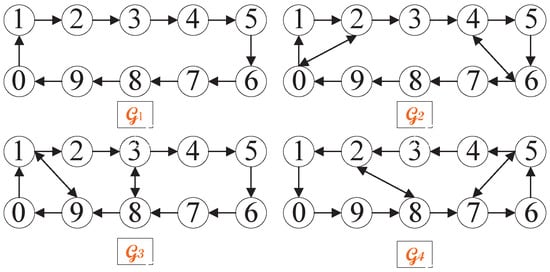
Figure 1. The directed communication graphs.

The parameters in Theorem 1 are selected as $q=0.5$, $\alpha =0.08$, and $\beta =1$. Furthermore, the nonlinear function is shown as $g\left(x_i(t-d\left(t\right))\right)=0.5\ast sin\left(x_i(t-d\left(t\right))\right)$, and the state delay is allowed to be $d\left(t\right)=0.04{sin}^2\left(t\right)+0.01$. In addition, we have $\dot{d}\left(t\right)=0.04sin\left(2t\right)$, and it can easily be obtained that $k=0.05$, ${\widehat{\mu }}_1=-0.04$ and ${\mu }_1=0.04$. Moreover, the communication delay is selected as $\tau \left(t\right)=0.03sin\left(t\right)+0.01$, and we have $h=0.04$ and ${\mu }_2=0.03$. Then, by solving the LMIs (7a)–(7d) in MATLAB, we can get

$$\begin{array}{c}\hfill P_1=\left[\begin{array}{cccccccccc}0.414& 0.111& 0.069& 0.012& 0.012& 0.007& 0.035& 0.075& 0.034& 0.161\\ 0.111& 0.279& 0.170& 0.036& 0.024& 0.019& 0.055& 0.182& 0.006& 0.049\\ 0.069& 0.170& 0.469& 0.171& 0.034& 0.022& 0.008& -0.009& -0.016& 0.012\\ 0.012& 0.036& 0.171& 0.421& 0.123& 0.081& 0.067& 0.016& -0.007& 0.010\\ 0.012& 0.024& 0.034& 0.123& 0.306& 0.209& 0.190& 0.003& 0.022& 0.007\\ 0.007& 0.019& 0.022& 0.081& 0.209& 0.423& 0.113& 0.028& 0.014& 0.014\\ 0.035& 0.055& 0.008& 0.067& 0.190& 0.113& 0.271& 0.114& 0.060& 0.017\\ 0.075& 0.182& -0.009& 0.016& 0.003& 0.028& 0.114& 0.284& 0.184& 0.054\\ 0.034& 0.006& -0.016& -0.007& 0.022& 0.014& 0.060& 0.184& 0.464& 0.169\\ 0.161& 0.049& 0.012& 0.010& 0.007& 0.014& 0.017& 0.054& 0.169& 0.437\end{array}\right],\end{array}$$

$$\begin{array}{c}\hfill P_2=\left[\begin{array}{cccccccccc}3.019& 0.287& 0.158& 0.015& 0.048& 0.014& 0.081& 0.181& -0.003& 0.443\\ 0.287& 2.083& 0.680& -0.030& 0.137& 0.006& 0.084& 1.071& -0.248& 0.171\\ 0.158& 0.680& 3.005& 0.473& 0.021& 0.056& 0.008& -0.266& 0.110& -0.003\\ 0.015& -0.030& 0.473& 3.018& 0.362& 0.118& 0.117& 0.128& -0.027& 0.068\\ 0.048& 0.137& 0.021& 0.362& 2.225& 0.677& 0.875& -0.244& 0.133& 0.007\\ 0.014& 0.006& 0.056& 0.118& 0.677& 2.951& 0.187& 0.160& 0.005& 0.066\\ 0.081& 0.084& 0.008& 0.117& 0.875& 0.187& 2.247& 0.526& 0.090& 0.026\\ 0.181& 1.071& -0.266& 0.128& -0.244& 0.160& 0.526& 1.973& 0.742& -0.031\\ -0.003& -0.248& 0.110& -0.027& 0.133& 0.005& 0.090& 0.742& 2.973& 0.467\\ 0.443& 0.171& -0.003& 0.069& 0.007& 0.066& 0.026& -0.031& 0.467& 3.027\end{array}\right],\end{array}$$

$$\begin{array}{c}\hfill Q_1=\left[\begin{array}{cccccccccc}0.922& 0.112& 0.119& 0.092& 0.094& 0.085& 0.077& 0.130& 0.100& 0.147\\ 0.112& 0.729& 0.204& 0.072& 0.141& 0.070& 0.086& 0.295& 0.022& 0.146\\ 0.119& 0.204& 0.876& 0.161& 0.091& 0.110& 0.096& 0.019& 0.131& 0.072\\ 0.092& 0.072& 0.161& 0.928& 0.146& 0.101& 0.108& 0.119& 0.060& 0.093\\ 0.094& 0.141& 0.091& 0.146& 0.804& 0.200& 0.198& 0.011& 0.126& 0.067\\ 0.085& 0.070& 0.110& 0.101& 0.200& 0.901& 0.092& 0.155& 0.078& 0.087\\ 0.077& 0.086& 0.096& 0.108& 0.197& 0.092& 0.861& 0.171& 0.080& 0.108\\ 0.130& 0.295& 0.019& 0.119& 0.011& 0.155& 0.171& 0.671& 0.235& 0.072\\ 0.100& 0.022& 0.131& 0.060& 0.126& 0.078& 0.080& 0.235& 0.875& 0.170\\ 0.147& 0.146& 0.072& 0.093& 0.067& 0.087& 0.108& 0.072& 0.170& 0.915\end{array}\right],\end{array}$$

$$\begin{array}{c}\hfill W_1=\left[\begin{array}{cccccccccc}3.149& -0.053& 0.022& -0.030& 0.019& -0.024& -0.020& 0.073& -0.061& 0.042\\ -0.053& 2.446& 0.349& -0.152& 0.201& -0.121& -0.105& 0.791& -0.383& 0.145\\ 0.022& 0.349& 3.016& 0.086& -0.098& 0.034& 0.015& -0.372& 0.154& -0.088\\ -0.030& -0.152& 0.086& 3.129& 0.058& -0.036& -0.022& 0.140& -0.084& 0.027\\ 0.019& 0.201& -0.098& 0.058& 2.716& 0.223& 0.332& -0.402& 0.140& -0.071\\ -0.024& -0.121& 0.034& -0.036& 0.223& 3.074& -0.136& 0.169& -0.088& 0.023\\ -0.020& -0.105& 0.015& -0.022& 0.332& -0.136& 2.874& 0.256& -0.092& 0.015\\ 0.073& 0.791& -0.372& 0.140& -0.402& 0.169& 0.256& 2.213& 0.453& -0.204\\ -0.061& -0.383& 0.154& -0.084& 0.140& -0.088& -0.092& 0.453& 2.968& 0.110\\ 0.042& 0.145& -0.088& 0.027& -0.071& 0.023& 0.015& -0.204& 0.110& 3.117\end{array}\right],\end{array}$$

$$\begin{array}{c}\hfill T_1=\left[\begin{array}{cccccccccc}2.305& 0.865& 0.569& -0.200& -0.137& -0.153& 0.118& 0.490& -0.002& 1.285\\ 0.865& 1.742& 1.397& 0.175& -0.143& -0.166& 0.337& 0.921& -0.170& 0.180\\ 0.569& 1.397& 3.468& 1.435& 0.096& 0.034& -0.274& -0.428& -1.006& -0.151\\ -0.200& 0.175& 1.435& 2.336& 0.948& 0.852& 0.525& -0.282& -0.421& -0.228\\ -0.137& -0.143& 0.096& 0.948& 1.918& 1.810& 1.054& -0.132& -0.079& -0.197\\ -0.153& -0.166& 0.034& 0.852& 1.810& 2.407& 0.752& -0.094& -0.156& -0.146\\ 0.118& 0.337& -0.274& 0.525& 1.054& 0.752& 1.436& 0.725& 0.519& -0.053\\ 0.490& 0.921& -0.428& -0.282& -0.132& -0.094& 0.725& 1.898& 1.631& 0.410\\ -0.002& -0.170& -1.006& -0.421& -0.079& -0.156& 0.519& 1.631& 3.420& 1.402\\ 1.285& 0.180& -0.151& -0.228& -0.197& -0.146& -0.053& 0.410& 1.402& 2.637\end{array}\right],\end{array}$$

$$\begin{array}{c}\hfill Q_{11}=\left[\begin{array}{cccccccccc}12.746& -2.556& -0.707& -0.602& 0.169& 0.113& -0.951& 0.586& -0.634& -1.654\\ -2.556& 14.129& -0.375& -0.825& -0.910& -1.420& 1.566& -1.542& -1.837& 0.280\\ -0.707& -0.375& 12.459& -1.587& 0.067& 0.036& -1.154& -1.407& -0.042& -0.780\\ -0.602& -0.825& -1.587& 12.533& -2.336& -2.336& 0.893& 0.893& -0.480& -0.059\\ 0.169& -0.910& 0.067& -2.336& 13.892& 0.632& -3.327& -0.990& -0.177& -0.508\\ 0.113& -1.420& 0.036& -2.336& 0.632& 13.227& -4.205& 0.214& -0.689& -0.252\\ -0.951& 1.566& -1.154& 0.893& -3.327& -4.205& 16.931& -2.366& -2.366& 0.002\\ 0.586& -1.542& -1.407& 0.893& -0.990& 0.214& -2.366& 13.638& 0.064& -1.809\\ -0.634& -1.837& -0.042& -0.480& -0.177& -0.689& -0.876& 0.064& 12.353& -1.171\\ -1.654& 0.280& -0.780& -0.059& -0.508& -0.252& 0.002& -1.809& -1.171& 12.463\end{array}\right],\end{array}$$

$$\begin{array}{c}\hfill Q_{22}=\left[\begin{array}{cccccccccc}7.203& 0.706& 0.548& 0.198& 0.210& 0.196& 0.341& 0.567& 0.388& 0.928\\ 0.706& 6.923& 0.939& 0.406& 0.250& 0.229& 0.448& 0.722& 0.250& 0.410\\ 0.548& 0.939& 7.760& 1.019& 0.392& 0.362& 0.211& 0.093& -0.222& 0.181\\ 0.198& 0.406& 1.019& 7.256& 0.789& 0.746& 0.562& 0.146& 0.026& 0.134\\ 0.210& 0.250& 0.392& 0.789& 7.060& 1.166& 0.812& 0.226& 0.215& 0.163\\ 0.196& 0.229& 0.362& 0.746& 1.166& 7.302& 0.696& 0.235& 0.174& 0.178\\ 0.341& 0.448& 0.211& 0.562& 0.812& 0.696& 6.805& 0.611& 0.611& 0.277\\ 0.567& 0.722& 0.093& 0.146& 0.226& 0.235& 0.611& 7.018& 1.098& 0.569\\ 0.388& 0.250& -0.222& 0.026& 0.215& 0.174& 0.611& 1.098& 7.788& 1.046\\ 0.928& 0.410& 0.181& 0.134& 0.163& 0.178& 0.277& 0.569& 1.046& 7.399\end{array}\right].\end{array}$$

Clearly, Figure 2 shows that the average consensus is achieved with $g\left(x_i(t-d\left(t\right))\right)=0.5\ast sin\left(x_i(t-d\left(t\right))\right)$. When $d\left(t\right)=0$, and we have $g\left(x_i\left(t\right)\right)=0.5\ast sin\left(x_i\left(t\right)\right)$; then, the average consensus is solved with only communication delay $\tau \left(t\right)$ in Figure 3. Furthermore, the trajectories of control inputs in Theorem 1 and in [28] are respectively presented in Figure 4 and Figure 5. Moreover, when $g\left(x_i(t-d\left(t\right))\right)=0$, as can be seen in Figure 6, the states of all agents eventually converge to zero, satisfying the initial condition ${\sum }_{i=1}^N{x}_i\left(0\right)=0$ in [28]. Based on the analysis and discussion above, we find that the convergence rates of state curves and control inputs in Theorem 1 are slower than those in [28] owing to the mixed TVDs. Thus, it appears that the average consensus problem for nonlinear MASs (1) with mixed TVDs via the PD protocol (2) has been solved under switching directed graphs.

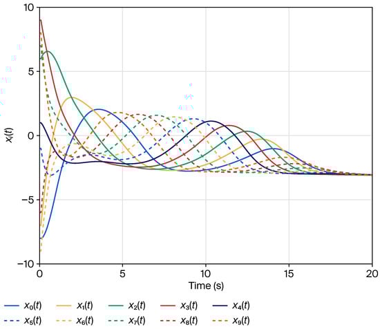
Figure 2. Trajectories of the agent state $x_i\left(t\right)$, $i\in \left\{1,2,\dots ,10\right\}$ in Theorem 1.

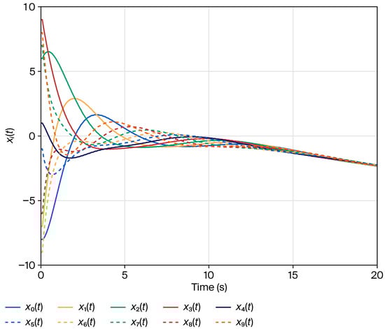
Figure 3. Trajectories of the agent state $x_i\left(t\right)$, $i\in \left\{1,2,\dots ,10\right\}$ when $d\left(t\right)=0$.

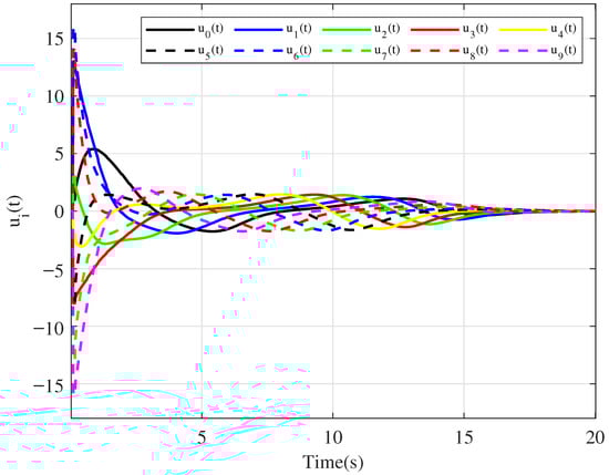
Figure 4. Control inputs of the agents in Theorem 1.

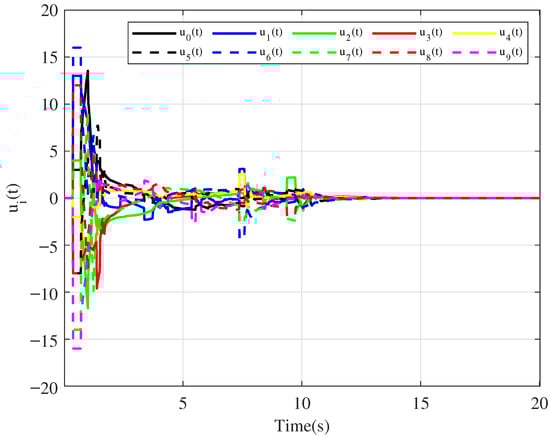
Figure 5. Control inputs of the agents in [28].

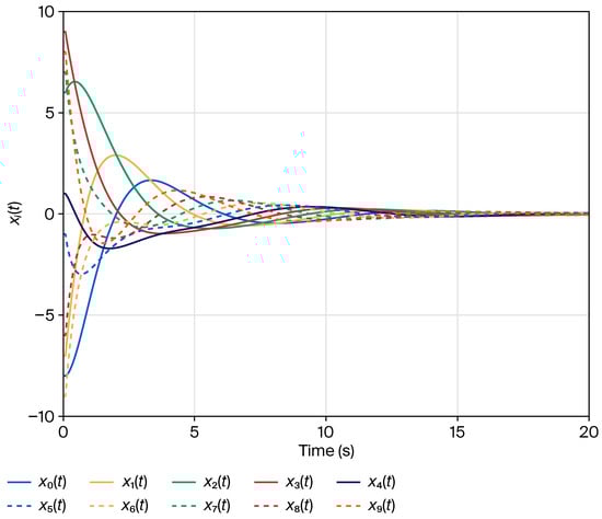
Figure 6. Trajectories of the agent state $x_i\left(t\right)$, $i\in \left\{1,2,\dots ,10\right\}$ when $g\left(x_i(t-d\left(t\right))\right)=0$ in [28].

5. Conclusions

Described by fast switching balanced digraphs, the distributed average consensus problems of nonlinear MASs with delays have been discussed. In light of mixed TVDs and their inherent nonlinearities, a distributed PD control algorithm is employed to address these concerns. Given the realities mentioned above, namely that the delays in this paper are varying and nonuniform, by designing novel LKFs containing both double- and triple-integral terms, the resulting conditions for the achievement of average consensus have been developed based on the LMI method. Numerical simulations validating the control scheme have been proposed. Based on these results, future works could include investigations into event-triggered optimal consensus problems of complex MASs with mixed TVDs and cyber-attacks on communication channels [47,48,49,50].

References

- Liu, Y.; Wang, Y.; Li, Y.; Gooi, H.; Xin, H. Multi-agent based optimal scheduling and trading for multi-microgrids integrated with urban transportation networks. IEEE Trans. Power Syst. 2021, 36, 2197–2210. [Google Scholar] [CrossRef]
- Mahela, O.; Khosravy, M.; Gupta, N.; Khan, B.; Alhelou, H.; Mahla, R.; Patel, N.; Siano, P. Comprehensive overview of multi-agent systems for controlling smart grids. CSEE J. Power Energy Syst. 2020, 8, 115–131. [Google Scholar] [CrossRef]
- Zhou, L.; Deng, X.; Wang, Z.; Zhang, X.; Dong, Y.; Hu, X.; Ning, Z.; Wei, J. Semantic information extraction and multi-agent communication optimization based on generative pre-trained transformer. IEEE Trans. Cogn. Commun. Netw. 2025, 11, 725–737. [Google Scholar] [CrossRef]
- Hou, Y.; Zhao, J.; Zhang, R.; Cheng, X.; Yang, L. UAV swarm cooperative target search: A multi-agent reinforcement learning approach. IEEE Trans. Intell. Veh. 2024, 9, 568–578. [Google Scholar] [CrossRef]
- Shi, P.; Yu, J. Dissipativity-based consensus for fuzzy multiagent systems under switching directed topologies. IEEE Trans. Fuzzy Syst. 2021, 29, 1143–1151. [Google Scholar] [CrossRef]
- Zhou, T.; Liu, Q.; Wang, W. Nonfragile containment control of nonlinear multi-agent systems via a disturbance observer-based approach. Int. J. Robust Nonlinear Control 2024, 34, 3726–3741. [Google Scholar] [CrossRef]
- Zhou, T.; Liu, C.; Wang, W. Nonfragile robust H∞ containment control for multi-agent systems with a time-varying delay. J. Frankl. Inst. 2024, 361, 106732. [Google Scholar] [CrossRef]
- Du, Z.; Xie, X.; Qu, Z.; Hu, Y.; Stojanovic, V. Dynamic event-triggered consensus control for interval type-2 fuzzy multi-agent systems. IEEE Trans. Circuits Syst. I Regul. Pap. 2024, 71, 3857–3866. [Google Scholar] [CrossRef]
- Liao, Z.; Wang, S.; Shi, J.; Haesaert, S.; Zhang, Y.; Sun, Z. Resilient containment under time-varying networks with relaxed graph robustness. IEEE Trans. Netw. Sci. Eng. 2024, 11, 4093–4105. [Google Scholar] [CrossRef]
- Yuan, T.; Li, L. Observer-based consensus control for a class of nonlinear singular multi-agent systems. J. Frankl. Inst. 2024, 361, 107061. [Google Scholar] [CrossRef]
- Sun, Y.; Wang, L.; Xie, G. Average consensus in networks of dynamic agents with switching topologies and multiple time-varying delays. Syst. Control Lett. 2008, 57, 175–183. [Google Scholar] [CrossRef]
- Wen, G.; Yu, W.; Xia, Y.; Yu, X.; Hu, J. Distributed tracking of nonlinear multiagent systems under directed switching topology: An observer-based protocol. IEEE Trans. Syst. Man Cybern. Syst. 2017, 47, 869–881. [Google Scholar] [CrossRef]
- Chen, L.; Mei, J.; Li, C.; Ma, G. Distributed leader-follower affine formation maneuver control for high-order multiagent systems. IEEE Trans. Autom. Control 2020, 65, 4941–4948. [Google Scholar] [CrossRef]
- Cui, Y.; Xu, J.; Xing, W.; Huang, F.; Yan, Z.; Du, X. Anti-disturbance cooperative formation containment control for multiple autonomous underwater vehicles with collision-free and actuator saturation constraints. J. Frankl. Inst. 2024, 361, 107063. [Google Scholar] [CrossRef]
- Dey, S.; Xu, H. Distributed adaptive flocking control for large-scale multiagent systems. IEEE Trans. Neural Networks Learn. Syst. 2025, 36, 3126–3135. [Google Scholar] [CrossRef] [PubMed]
- Xiao, L.; Boyd, S.; Kim, S. Distributed average consensus with least-mean-square deviation. IEEE Trans. Fuzzy Syst. 2007, 67, 33–46. [Google Scholar] [CrossRef]
- Liu, J.; Yu, Y.; Xu, Y.; Zhang, Y.; Sun, C. Fixed-time average consensus of nonlinear delayed MASs under switching topologies: An event-based triggering approach. IEEE Trans. Syst. Man Cybern. Syst. 2022, 52, 2721–2733. [Google Scholar] [CrossRef]
- Guo, W.; Shi, L.; Sun, W.; Jahanshahi, H. Predefined-time average consensus control for heterogeneous nonlinear multi-agent systems. IEEE Trans. Circuits Syst. II Express Briefs 2023, 70, 2989–2993. [Google Scholar] [CrossRef]
- Liu, L.; Cao, J.; Alsaadi, F. Aperiodically intermittent event-triggered optimal average consensus for nonlinear multi-agent systems. IEEE Trans. Neural Networks Learn. Syst. 2024, 35, 10338–10352. [Google Scholar] [CrossRef]
- Hui, M.; Liu, X.; Cao, J. Improved fixed-time event-triggered average consensus of multi-agent systems under DoS attacks. IEEE Trans. Circuits Syst. II Express Briefs 2024, 71, 3815–3819. [Google Scholar] [CrossRef]
- Martinez, G.; Orchard, M.; Bozhko, S. Dynamic average consensus with anti-windup applied to interlinking converters in AC/DC microgrids under economic dispatch and delays. IEEE Trans. Smart Grid 2023, 14, 4137–4140. [Google Scholar] [CrossRef]
- Sun, F.; Guan, Z.; Ding, L.; Wang, Y. Mean square average-consensus for multi-agent systems with measurement noise and time delay. Int. J. Syst. Sci. 2013, 44, 995–1005. [Google Scholar] [CrossRef]
- Liu, C.; Shan, L.; Chen, Y.; Zhang, Y. Average-consensus filter of first-order multi-agent systems with disturbances. IEEE Trans. Circuits Syst. II Express Briefs 2018, 65, 1763–1767. [Google Scholar] [CrossRef]
- Aragues, R.; González, A.; López-Nicolás, G.; Sagues, C. Convergence speed of dynamic consensus with delay compensation. Neurocomputing 2024, 570, 127130. [Google Scholar] [CrossRef]
- Chen, C.; Wen, G.; Liu, Y.; Wang, F. Adaptive consensus control for a class of nonlinear multiagent time-delay systems using neural networks. IEEE Trans. Neural Networks Learn. Syst. 2014, 25, 1217–1226. [Google Scholar] [CrossRef]
- Ma, H.; Wang, Z.; Wang, D.; Liu, D.; Yan, P.; Wei, Q. Neural-network-based distributed adaptive robust control for a class of nonlinear multiagent systems with time delays and external noises. IEEE Trans. Syst. Man Cybern. Syst. 2016, 46, 750–758. [Google Scholar] [CrossRef]
- Wen, G.; Chen, C.; Liu, Y.; Liu, Z. Neural network-based adaptive leader-following consensus control for a class of nonlinear multiagent state-delay systems. IEEE Trans. Cybern. 2017, 47, 2151–2160. [Google Scholar] [CrossRef] [PubMed]
- Wang, D.; Zhang, N.; Wang, J.; Wang, W. A PD-like protocol with a time delay to average consensus control for multi-agent systems under an arbitrarily fast switching topology. IEEE Trans. Cybern. 2017, 47, 898–907. [Google Scholar] [CrossRef]
- Qian, W.; Gao, Y.; Wang, L.; Fei, S. Consensus of multiagent systems with nonlinear dynamics and time-varying communication delays. Int. J. Robust Nonlinear Control 2019, 29, 1926–1940. [Google Scholar] [CrossRef]
- Ma, D.; Chen, J.; Lu, R.; Chen, J.; Chai, T. Delay consensus margin of first-order multiagent systems with undirected graphs and PD protocols. IEEE Trans. Autom. Control 2021, 66, 4192–4198. [Google Scholar] [CrossRef]
- Ma, D. Delay range for consensus achievable by proportional and PD feedback protocols with time-varying delays. IEEE Trans. Autom. Control 2022, 67, 3212–3219. [Google Scholar] [CrossRef]
- Caiazzo, B.; Lui, D.; Petrillo, A.; Santini, S. Signed average consensus in cooperative-antagonistic multi-agent systems with multiple communication time-varying delays. IFAC 2024, 58, 114–119. [Google Scholar] [CrossRef]
- Tang, Z.; Wang, K.; Feng, J.; Park, J. Edge-based self-triggering impulsive consensus on nonlinear multi-agent systems with proportional delay. IEEE Trans. Autom. Sci. Eng. 2024, 21, 7494–7504. [Google Scholar] [CrossRef]
- Peng, X.; He, Y. Consensus of multiagent systems with time-varying delays and switching topologies based on delay-product-type functionals. IEEE Trans. Cybern. 2024, 54, 101–110. [Google Scholar] [CrossRef] [PubMed]
- Zhou, T. H∞ containment control of multi-agent systems with mixed time-varying delays and exogenous disturbances via observer-based output feedback. Asian J. Control 2025, 1–11. [Google Scholar] [CrossRef]
- Peng, X.; He, Y.; Liu, Z.; You, L.; Li, H. Time-varying formation H∞ tracking control and optimization for delayed multi-agent systems with exogenous disturbances. IEEE Trans. Autom. Sci. Eng. 2025, 22, 5637–5647. [Google Scholar] [CrossRef]
- Liu, Y.; Zhang, C.; Shangguan, X.; Chen, J.; He, Y. H∞-based tracking control for nonlinear systems with a sampled-data PI-type controller: A nonuniform sampled-time-dependent functional. IEEE Trans. Cybern. 2025, 55, 4286–4299. [Google Scholar] [CrossRef]
- Yang, Y.; He, Y. Time-varying formation-containment control for heterogeneous multi-agent systems with communication and output delays via observer-based feedback protocol. IEEE Trans. Autom. Sci. Eng. 2025, 22, 15435–15448. [Google Scholar] [CrossRef]
- Zhai, Z.; Yan, H.; Chen, S.; Chang, Y.; Shi, K. Nonlinear multi-agent systems consensus via delayed non-fragile sampled-data control. IEEE Trans. Control Netw. Syst. 2025, 12, 275–286. [Google Scholar] [CrossRef]
- Zhang, W.; Chen, J.; Wen, S.; Huang, T. Event-triggered random delayed impulsive consensus of multi-agent systems with time-varying delay. IEEE Trans. Emerg. Top. Comput. Intell. 2025, 9, 2059–2064. [Google Scholar] [CrossRef]
- Tang, Z.; Zhen, Z.; Zhao, Z.; Deconinck, G. Observer-based resilient PD-like scaled group consensus for uncertain multiagent systems under time-varying delays. Commun. Nonlinear Sci. Numer. Simul. 2025, 148, 108846. [Google Scholar] [CrossRef]
- Aghayan, Z.; Alfi, A.; Mousavi, Y.; Fekih, A. Robust delay-dependent output-feedback PD controller design for variable fractional-order uncertain neutral systems with time-varying delays. IEEE Trans. Syst. Man Cybern. Syst. 2025, 55, 1986–1996. [Google Scholar] [CrossRef]
- Mesbahi, M.; Egerstedt, M. Graph Theoretic Methods in Multiagent Networks; Princeton University Press: Princeton, NY, USA, 2010. [Google Scholar]
- Bliman, P.; Ferrari-Trecate, G. Average consensus problems in networks of agents with delayed communications. Automatica 2008, 44, 1985–1995. [Google Scholar] [CrossRef]
- Lin, P.; Jia, Y.; Li, L. Distributed robust H∞ consensus control in directed networks of agents with time-delay. Syst. Control Lett. 2008, 57, 643–653. [Google Scholar] [CrossRef]
- Sun, J.; Liu, G.; Chen, J. Delay-dependent stability and stabilization of neutral time-delay systems. Int. J. Robust Nonlinear Control 2009, 19, 1364–1375. [Google Scholar] [CrossRef]
- Wang, D.; Zhou, J.; Wen, G.; Lü, J.; Chen, G. Event-triggered optimal consensus of second-order MASs with disturbances and cyber attacks on communications edges. IEEE Trans. Netw. Sci. Eng. 2023, 10, 3846–3857. [Google Scholar] [CrossRef]
- Hu, T.; Song, Q.; Zhang, X.; Shi, K. Hybrid event-triggered and impulsive security consensus control strategy for fractional-order multiagent systems with cyber attacks. IEEE Trans. Syst. Man Cybern. Syst. 2025, 55, 830–842. [Google Scholar] [CrossRef]
- Zhang, T.; Ye, D.; Shi, Y. Decentralized false-data injection attacks against state omniscience: Existence and security analysis. IEEE Trans. Autom. Control 2023, 68, 4634–4649. [Google Scholar] [CrossRef]
- Zhang, T.; Ye, D.; Yang, G. Ripple effect of cooperative attacks in multi-agent systems: Results on minimum attack targets. Automatica 2024, 159, 111307. [Google Scholar] [CrossRef]
Disclaimer/Publisher’s Note: The statements, opinions and data contained in all publications are solely those of the individual author(s) and contributor(s) and not of MDPI and/or the editor(s). MDPI and/or the editor(s) disclaim responsibility for any injury to people or property resulting from any ideas, methods, instructions or products referred to in the content. |
© 2025 by the author. Licensee MDPI, Basel, Switzerland. This article is an open access article distributed under the terms and conditions of the Creative Commons Attribution (CC BY) license (https://creativecommons.org/licenses/by/4.0/).