A High-Order Proper Orthogonal Decomposition Dimensionality Reduction Compact Finite-Difference Method for Diffusion Problems

Abstract

An innovative high-order dimensionality reduction approach, which integrates a condensed finite-difference scheme with proper orthogonal decomposition techniques, has been explored for solving diffusion equations. The difference scheme with forth order accurate in both space and time is introduced through the idea of interpolation approximation. The quartic spline function and $(2,2)$ Padé approximation were utilized in space and time discretization, respectively. The stability and convergence were proven. Moreover, the dimensionality reduction formulas were derived using the proper orthogonal decomposition (POD) method, which is based on the matrix representation of the compact finite-difference scheme. The bases of the POD method were established by cumulative contribution rate of the eigenvalues of snapshot matrix that is different from the traditional ways in which the bases were established by the first eigenvalues. The method of cumulative contribution rate can optimize the degree of freedom. The error analysis of the reduced bases high-order POD finite-difference scheme was provided. Numerical experiments are conducted to validate the soundness and dependability of the reduced-order algorithm. The comparisons between the $(2,2)$ finite-difference method, the traditional POD method, and reduced dimensional method with cumulative contribution rate were discussed.

1. Introduction

The diffusion equation, a parabolic partial differential equation, characterizes how physical quantities spread and dissipate over time. The diffusion equation is capable of describing a wide range of physical phenomena that occur in natural environments, engineering systems, and biological organisms. These phenomena include gas diffusion, heat conduction, liquid permeation, and impurity diffusion in semiconductor materials. Due to the complexity of the physical problems themselves, their exact solutions are not easy to obtain. Therefore, studying numerical methods to solve these problems holds significant value both theoretically and in engineering applications.

Over the past few decades, high-order compact difference methods have garnered renewed interest. Consequently, numerous specialized techniques have been developed. Lin [1] transformed the problem into a system of ordinary differential equations using the method of lines and Taylor series expansion, thereby proposing a sixth-order accurate finite-difference scheme. Zhao [2] constructed a combined difference scheme integrating treatments for both interior and boundary nodes specifically for heat conduction problems. Gao [3] semi-discretized the hyperbolic equation and transformed it into ordinary differential equations, thereby obtaining a novel finite-difference scheme. Liu’s work [4] presents two advanced numerical approaches combining temporal Padé discretization with spatial spline techniques. The $(3,3)$ Padé approximation technique was applied by Zhang [5] to spatial fractional equations. Concurrently, Chen’s group [6] achieved high-order accuracy in solving parabolic equations through innovative combinations of finite-difference schemes with Padé-based approximations.

Although the finite-difference method has been used for numerous problems and shows good simulation results, it often involves a large number of unknowns when applied to large-scale or complex engineering problems. The large number of degrees of freedom enhances the computational complexity and restricts practical applicability. Furthermore, solving large algebraic systems not only reduces computational efficiency but also increases memory consumption and error accumulation. Therefore, it becomes imperative to design a reduced-order difference extrapolation scheme that can minimize the number of unknowns while maintaining sufficiently high accuracy. This paper presents for the first time a novel high-order reduced-dimensional compact difference scheme that innovatively integrates a difference scheme, the POD, and the cumulative contribution rate method for solving diffusion equations.

For dimensionality reduction purposes, the proper orthogonal decomposition (POD) method proves highly effective in approximating large-scale datasets. It can save storage space, optimize computations, and reduce CPU time. The method has been extensively used in solving partial differential equations numerically [7,8,9], and has found applications in a wide range of fields, including turbulence analysis [10,11], atmospheric modeling [12], and geophysics [13], among others. For example, Sun [14] was the first to integrate the POD method with the FD method, resulting in a POD-based dimensionality reduction scheme for parabolic equations. In [15], a reduced-order FD scheme was developed for the Richards equation, and its convergence and stability were analyzed. Luo [16] constructed a POD reduced-order scheme for the non-stationary Stokes equations. Using SVD and POD, Hong et al. [17] developed a reduced-order method for the Sobolev equation. In [18], Deng and colleagues introduced a dimensionality reduction approach for hyperbolic equations in two dimensions, employing POD techniques. Ren [19] constructed a POD-based dimensionality reduction scheme for spatial fractional parabolic equations. In addition, the dimensionality reduction method of proper orthogonal decomposition (POD) is also combined with other traditional numerical methods to construct reduced-order models. Notable examples include the POD-based finite volume element scheme [20], the mixed finite element formulation incorporating POD [21,22], the space–time POD element technique [23,24], and reduced-order spectral methods [25,26], among others.

However, to date, no studies have reported the construction of reduced-order finite-difference schemes by combining the cumulative contribution rate method with POD. This study proposes a novel dimensionality reduction method that integrates finite-difference schemes with proper orthogonal decomposition (POD) techniques and the cumulative contribution rate method for solving diffusion equations. This study develops a fourth-order accurate FD scheme in both time and space dimensions through interpolation-based approximation techniques. The quartic spline function and $(2,2)$ Padé approximation were utilized in space and time discretization, respectively. The stability and convergence were proven. Furthermore, the dimensionality reduction formulas were obtained by POD method based on the matrix form of compact finite-difference scheme. This paper first establishes the theoretical foundation of the POD method through the eigenvalues of the snapshot matrix and then conducts an error analysis of the resulting POD-based reduced-order scheme. Then, based on this approach, we derive new basis functions for the POD method by calculating the cumulative contribution rate of the eigenvalues of the snapshot matrix. Unlike the traditional method of establishing the basis using the first eigenvalues, this method can optimize the degrees of freedom. The rationality and reliability of the reduced-order algorithm are verified through numerical experiments. The comparisons between the $(2,2)$ finite-difference method, the traditional POD method, and the reduced method with cumulative contribution rate were discussed. Consequently, by leveraging proper orthogonal decomposition and considering the cumulative contribution threshold, we formulate a novel implicit numerical approach with enhanced precision for this class of equations. Subsequently, we analyze the error estimation of the scheme. Finally, the consistency of the method with the theory was verified through two numerical examples, and its significant advantages over the classical finite-difference scheme were demonstrated.

The subsequent sections of this article are arranged as follows. In Section 2, the finite-difference method is introduced. In Section 3, the uniqueness and stability of the solution of this finite-difference scheme are proven. In Section 4, the concept of cumulative contribution rate is introduced, and a new POD basis is constructed. Building upon the optimized POD technique, we propose a novel reduced-order finite-difference scheme and provide its corresponding error analysis. The numerical validation presented in Section 5 confirms the practical viability and computational efficiency of the developed approach. Finally, Section 6 summarizes the research findings of this paper and further discusses potential future research directions.

2. Finite-Difference (FD) Scheme

The problem investigated in this paper is formulated as follows:

$$\left\{\begin{array}{ccc}\hfill & {\displaystyle \frac{\partial u}{\partial t}}=a\left({\displaystyle \frac{{\partial }^{2}u}{\partial x^2}}+{\displaystyle \frac{{\partial }^{2}u}{\partial y^2}}\right),\hfill & \hfill x,y\in [0,1],t\in (0,T],\\ \hfill & u(x,y,0)=p(x,y),\hfill & \hfill x,y\in [0,1],\\ \hfill & u(0,y,t)=0,u(1,y,t)=0,\hfill & \hfill t\in (0,T],\\ \hfill & u(x,0,t)=0,u(x,1,t)=0,\hfill & \hfill t\in (0,T].\end{array}\right.$$

(1)

where $0<x,y<1$, $t>0$, $a>0$ represents the diffusion coefficient, u is an unknown quantity, and $p(x,y)$ is a sufficiently smooth function.

For simplicity, let us assume that the mesh is equidistant. Namely, let ${\Pi }_x$ and ${\Pi }_y$ be the partitions in the x and y directions on the interval $[0,1]$, that is

$${\Pi }_x:0=x_0<x_1<\cdots <x_N=1,$$

$${\Pi }_y:0=y_0<y_1<\cdots <y_N=1,$$

where $h_x=h_y=h={\displaystyle \frac{1}{N}}$, $x_i=ih$, $y_j=jh$, $i,j=0,1,\dots ,N$.

Define the following spline function space

$$S_4^3(\Pi )=\left\{s\left(x\right)\in C^3[a,b]|s\left(x\right)\in P_4,x\in [x_{i-1},x_i],i=1,2,\dots ,N\right\}.$$

Here, $P_4$ denotes the set of polynomials with degree no more than 4. For any $s\left(x\right)\in S_4^3(\Pi )$, within every subinterval $[x_{i-1},x_i]$ ($i=1,2,\dots ,N$), let

$$s\left(x\right)=a_i+b_{i}t+c_i{t}^2+d_i{t}^3+e_i{t}^4,$$

From reference [4], we get

$$s\left(x_{i+1}\right)-2s\left(x_i\right)+s\left(x_{i-1}\right)={\displaystyle \frac{h^2}{12}}[s^{″}\left(x_{i+1}\right)+10s^{″}\left(x_i\right)+s^{″}\left(x_{i-1}\right)].$$

(2)

That is

$${\displaystyle \frac{1}{h^2}}[s\left(x_{i+1}\right)-2s\left(x_i\right)+s\left(x_{i-1}\right)]={\displaystyle \frac{1}{12}}[s^{″}\left(x_{i+1}\right)+10s^{″}\left(x_i\right)+s^{″}\left(x_{i-1}\right)],i=0,1,2,\dots$$

We denote $D^{\left(i\right)}s\left(x\right)=s^{\left(i\right)}\left(x\right)$. Here, $D^{\left(i\right)}$ is the differential.

Then, from reference [4], we get

$$\begin{array}{cc}\hfill s\left(x_{i+1}\right)& =s\left(x_i\right)+h{s}^{\prime }\left(x_i\right)+{\displaystyle \frac{1}{2}}{h}^2{s}^{″}\left(x_i\right)+\cdots =e^{hD}s\left(x_i\right),\hfill \\ \hfill s\left(x_{i-1}\right)& =s\left(x_i\right)-h{s}^{\prime }\left(x_i\right)+{\displaystyle \frac{1}{2}}{h}^2{s}^{″}\left(x_i\right)-\cdots =e^{-hD}s\left(x_i\right).\hfill \end{array}$$

Equation (2) can be written as

$${\displaystyle \frac{1}{h^2}}[e^{hD}-2+e^{-hD}]s\left(x_i\right)={\displaystyle \frac{1}{12}}[e^{hD}+10+e^{-hD}]s^{″}\left(x_i\right).$$

(3)

Theorem 1. 

If $f\left(x\right)$ is sufficiently smooth on $[a,b]$, let $s\left(x\right)\in S_4^3(\Pi )$ be the spline interpolating $f\left(x\right)$, satisfying:

$$s\left(x_i\right)=f\left(x_i\right),i=0,1,\dots ,N,$$

(4)

$$s^{″}\left(x_N\right)=f^{″}\left(x_N\right),s^{\prime }\left(x_0\right)=f^{\prime }\left(x_0\right),s^{\prime }\left(x_N\right)=f^{\prime }\left(x_N\right).$$

Therefore, we have

$$s^{″}\left(x_i\right)=f^{″}\left(x_i\right)-{\displaystyle \frac{h^4}{240}}{f}^{\left(6\right)}\left(x_i\right)+O\left(h^6\right),i=1,\dots ,N-1,$$

(5)

Proof. 

From (3) and (4), we can obtain

$${\displaystyle \frac{1}{h^2}}[e^{hD}-2+e^{-hD}]f\left(x_i\right)={\displaystyle \frac{1}{12}}[e^{hD}+10+e^{-hD}]s^{″}\left(x_i\right),i=1,\dots ,N-1.$$

By performing a Taylor expansion of $e^{hD}$ and $e^{-hD}$, Equation (5) can be obtained. □

Assume that $u(x,y,t)$ is the exact solution to Equation (1). According to the quartic spline interpolation function, let $S_4^3\left({\Pi }_x\right)$ be the spline space on the partition ${\Pi }_x$. For any fixed y and t, the spline interpolation function $s(x,y_j,t_k)\in S_4^3\left({\Pi }_x\right)$ interpolates $u(x,y_j,t_k)$ and satisfies the following interpolation conditions

$$\begin{array}{cc}\hfill s(x_i,y_j,t_k)& =u(x_i,y_j,t_k),\hfill \\ \hfill s_x(x_0,y_j,t_k)& =u_x(x_0,y_j,t_k),\hfill \\ \hfill s_x(x_N,y_j,t_k)& =u_x(x_N,y_j,t_k),\hfill \\ \hfill s_{xx}(x_N,y_j,t_k)& =u_{xx}(x_N,y_j,t_k).\hfill \end{array}$$

(6)

Similarly, the same interpolation conditions are satisfied in the y direction.

According to Theorem 1, we get

$$s_{xx}(x_i,y_j,t_k)=u_{xx}(x_i,y_j,t_k)-{\displaystyle \frac{h^4}{240}}{\displaystyle \frac{{\partial }^{6}u(x_i,y_j,t_k)}{\partial x^6}}+O\left(h^6\right).$$

Similarly, for any fixed x and t, we have

$$s_{yy}(x_i,y_j,t_k)=u_{yy}(x_i,y_j,t_k)-{\displaystyle \frac{h^4}{240}}{\displaystyle \frac{{\partial }^{6}u(x_i,y_j,t_k)}{\partial y^6}}+O\left(h^6\right).$$

From Equation (2), we have

$$\begin{array}{cc}\hfill s(x_{i-1},y_j,t_k)-2s(x_i,y_j,t_k)+s(x_{i+1},y_j,t_k)& ={\displaystyle \frac{h^2}{12}}[s_{xx}(x_{i-1},y_j,t_k)+10s_{xx}(x_i,y_j,t_k)\hfill \\ \hfill & +s_{xx}(x_{i+1},y_j,t_k)],\hfill \end{array}$$

(7)

$$\begin{array}{cc}\hfill s(x_i,y_{j-1},t_k)-2s(x_i,y_j,t_k)+s(x_i,y_{j+1},t_k)& ={\displaystyle \frac{h^2}{12}}[s_{yy}(x_i,y_{j-1},t_k)+10s_{yy}(x_i,y_j,t_k)\hfill \\ \hfill & +s_{yy}(x_i,y_{j+1},t_k)].\hfill \end{array}$$

(8)

$$D_x^{i}s(x,y,t)={\displaystyle \frac{{\partial }^{i}s(x,y,t)}{\partial x^i}},i=0,1,2,\dots$$

Then

$$s(x_{i\pm 1},y_j,t_k)=s(x_i,y_j,t_k)\pm h{\displaystyle \frac{\partial s(x_i,y_j,t_k)}{\partial x}}+\cdots =e^{\pm h{D}_x}s(x_i,y_j,t_k),$$

$$s(x_i,y_{j\pm 1},t_k)=s(x_i,y_j,t_k)\pm h{\displaystyle \frac{\partial s(x_i,y_j,t_k)}{\partial y}}+\cdots =e^{\pm h{D}_y}s(x_i,y_j,t_k).$$

Then Equations (7) and (8) can be written as

$$(e^{h{D}_x}+10+e^{-h{D}_x})s_{xx}(x_i,y_j,t_k)={\displaystyle \frac{12}{h^2}}(e^{h{D}_x}-2+e^{-h{D}_x})s(x_i,y_j,t_k),$$

(9)

$$(e^{h{D}_y}+10+e^{-h{D}_y})s_{yy}(x_i,y_j,t_k)={\displaystyle \frac{12}{h^2}}(e^{h{D}_y}-2+e^{-h{D}_y})s(x_i,y_j,t_k).$$

Applying $(e^{h{D}_x}+10+e^{-h{D}_x})$ to Equation (7) and combining Equations (6) and (9), we get

$$\begin{array}{cc}\hfill (e^{h{D}_x}+10+e^{-h{D}_x})u_{xx}(x_i,y_j,t_k)& =(e^{h{D}_x}+10+e^{-h{D}_x})s_{xx}(x_i,y_j,t_k)+O\left(h^4\right)\hfill \\ & ={\displaystyle \frac{12}{h^2}}(e^{h{D}_x}-2+e^{-h{D}_x})s(x_i,y_j,t_k)+O\left(h^4\right)\hfill \\ & ={\displaystyle \frac{12}{h^2}}(e^{h{D}_x}-2+e^{-h{D}_x})u(x_i,y_j,t_k)+O\left(h^4\right).\hfill \end{array}$$

Neglecting the higher-order error terms, we obtain

$$(e^{h{D}_x}+10+e^{-h{D}_x})u_{xx}(x_i,y_j,t_k)={\displaystyle \frac{12}{h^2}}(e^{h{D}_x}-2+e^{-h{D}_x})u(x_i,y_j,t_k).$$

(10)

Similarly, we can obtain

$$(e^{h{D}_y}+10+e^{-h{D}_y})u_{yy}(x_i,y_j,t_k)={\displaystyle \frac{12}{h^2}}(e^{h{D}_y}-2+e^{-h{D}_y})u(x_i,y_j,t_k).$$

(11)

We define the following operators

$$\begin{array}{cc}\hfill L_{x1}& =e^{h{D}_x}+10+e^{-h{D}_x},\hfill \\ \hfill L_{y1}& =e^{h{D}_y}+10+e^{-h{D}_y},\hfill \\ \hfill L_{x2}& =e^{h{D}_x}-2+e^{-h{D}_x},\hfill \\ \hfill L_{y2}& =e^{h{D}_y}-2+e^{-h{D}_y}.\hfill \end{array}$$

Then Equations (10) and (11) can be rewritten as

$$L_{x1}{u}_{xx}(x_i,y_j,t_k)={\displaystyle \frac{12}{h^2}}{L}_{x2}u(x_i,y_j,t_k),$$

(12)

$$L_{y1}{u}_{yy}(x_i,y_j,t_k)={\displaystyle \frac{12}{h^2}}{L}_{y2}u(x_i,y_j,t_k).$$

(13)

Let

$$\begin{array}{cc}\hfill {\left(u_t\right)}_{i,j}\left(t\right)& =u_t(x_i,y_j,t),\hfill \\ \hfill {\left(u_{xx}\right)}_{i,j}\left(t\right)& =u_{xx}(x_i,y_j,t),\hfill \\ \hfill {\left(u_{yy}\right)}_{i,j}\left(t\right)& =u_{yy}(x_i,y_j,t).\hfill \end{array}$$

Applying the operator $L_{x1}{L}_{y1}$ to (1) and semidiscretizing it at point $(x_i,y_j,t)$, we have

$$L_{x1}{L}_{y1}{\left(u_t\right)}_{i,j}\left(t\right)=a{L}_{x1}{L}_{y1}{(u_{xx}+u_{yy})}_{i,j}\left(t\right).$$

(14)

Substituting (12) and (13) into (14), we obtain

$$L_{x1}{L}_{y1}{\left(u_t\right)}_{i,j}\left(t\right)={\displaystyle \frac{12a}{h^2}}(L_{x2}{L}_{y1}+L_{x1}{L}_{y2})u_{i,j}\left(t\right).$$

Thus, we obtain the semi-discrete scheme of Equation (1)

$$\begin{array}{cc}\hfill & {\left(u_t\right)}_{i-1,j-1}\left(t\right)+10{\left(u_t\right)}_{i-1,j}\left(t\right)+{\left(u_t\right)}_{i-1,j+1}\left(t\right)\hfill \\ \hfill & +10{\left(u_t\right)}_{i,j-1}\left(t\right)+100{\left(u_t\right)}_{i,j}\left(t\right)+10{\left(u_t\right)}_{i,j+1}\left(t\right)\hfill \\ \hfill & +{\left(u_t\right)}_{i+1,j-1}\left(t\right)+10{\left(u_t\right)}_{i+1,j}\left(t\right)+{\left(u_t\right)}_{i+1,j+1}\left(t\right)\hfill \\ \hfill & ={\displaystyle \frac{24a}{h^2}}\left[u_{i-1,j-1}\left(t\right)+4u_{i-1,j}\left(t\right)+u_{i-1,j+1}\left(t\right)\right.\hfill \\ \hfill & \left.+4u_{i,j-1}\left(t\right)-20u_{i,j}\left(t\right)+4u_{i,j+1}\left(t\right)+u_{i+1,j-1}\left(t\right)+4u_{i+1,j}\left(t\right)+u_{i+1,j+1}\left(t\right)\right],\hfill \\ \hfill & i,j=1,2,\dots ,N-1.\hfill \end{array}$$

(15)

The above difference scheme can be written in matrix form as

$$\mathbf{D}{\displaystyle \frac{d}{dt}}\mathbf{U}\left(\mathbf{t}\right)=\mathbf{E}\mathbf{U}\left(\mathbf{t}\right),$$

(16)

where

$$\mathbf{D}={\left(\begin{array}{ccccccc}{\mathbf{D}}_1& {\mathbf{D}}_2& \mathbf{O}& \cdots & \mathbf{O}& \mathbf{O}& \mathbf{O}\\ {\mathbf{D}}_2& {\mathbf{D}}_1& {\mathbf{D}}_2& \cdots & \mathbf{O}& \mathbf{O}& \mathbf{O}\\ ⋮& ⋮& ⋮& & ⋮& ⋮& ⋮\\ \mathbf{O}& \mathbf{O}& \mathbf{O}& \cdots & {\mathbf{D}}_2& {\mathbf{D}}_1& {\mathbf{D}}_2\\ \mathbf{O}& \mathbf{O}& \mathbf{O}& \cdots & \mathbf{O}& {\mathbf{D}}_2& {\mathbf{D}}_1\end{array}\right)}_{{(N-1)}^2\times {(N-1)}^2},$$

$${\mathbf{D}}_1={\left(\begin{array}{ccccc}100& 10& 0& \cdots & 0\\ 10& 100& 10& \cdots & 0\\ 0& 10& 100& \cdots & 0\\ ⋮& ⋮& ⋮& \ddots & ⋮\\ 0& 0& 0& \cdots & 100\end{array}\right)}_{(N-1)\times (N-1)},$$

$${\mathbf{D}}_2={\left(\begin{array}{ccccc}10& 1& 0& \cdots & 0\\ 1& 10& 1& \cdots & 0\\ 0& 1& 10& \cdots & 0\\ ⋮& ⋮& ⋮& \ddots & ⋮\\ 0& 0& 0& \cdots & 10\end{array}\right)}_{(N-1)\times (N-1)},$$

$$\mathbf{E}={\displaystyle \frac{24a}{h^2}}{\left(\begin{array}{ccccccc}{\mathbf{E}}_1& {\mathbf{E}}_2& \mathbf{O}& \cdots & \mathbf{O}& \mathbf{O}& \mathbf{O}\\ {\mathbf{E}}_2& {\mathbf{E}}_1& {\mathbf{E}}_2& \cdots & \mathbf{O}& \mathbf{O}& \mathbf{O}\\ ⋮& ⋮& ⋮& & ⋮& ⋮& ⋮\\ \mathbf{O}& \mathbf{O}& \mathbf{O}& \cdots & {\mathbf{E}}_2& {\mathbf{E}}_1& {\mathbf{E}}_2\\ \mathbf{O}& \mathbf{O}& \mathbf{O}& \cdots & \mathbf{O}& {\mathbf{E}}_2& {\mathbf{E}}_1\end{array}\right)}_{{(N-1)}^2\times {(N-1)}^2},$$

$${\mathbf{E}}_1={\left(\begin{array}{ccccc}-20& 4& 0& \cdots & 0\\ 4& -20& 4& \cdots & 0\\ 0& 4& -20& \cdots & 0\\ ⋮& ⋮& ⋮& \ddots & ⋮\\ 0& 0& 0& \cdots & -20\end{array}\right)}_{(N-1)\times (N-1)},$$

$${\mathbf{E}}_2={\left(\begin{array}{ccccc}4& 1& 0& \cdots & 0\\ 1& 4& 1& \cdots & 0\\ 0& 1& 4& \cdots & 0\\ ⋮& ⋮& ⋮& \ddots & ⋮\\ 0& 0& 0& \cdots & 4\end{array}\right)}_{(N-1)\times (N-1)},$$

$$\mathbf{U}\left(\mathbf{t}\right)={\left(\begin{array}{ccccc}{\mathbf{u}}_1\left(t\right),& {\mathbf{u}}_2\left(t\right),& & \dots ,& {\mathbf{u}}_{N-1}\left(t\right)\end{array}\right)}^T,$$

$${\mathbf{u}}_i\left(t\right)={\left(\begin{array}{ccccc}{u}_{i,1}\left(t\right),& u_{i,2}\left(t\right),& & \dots ,& u_{i,N-1}\left(t\right)\end{array}\right)}^T.$$

Let $\mathbf{C}=-{\mathbf{D}}^{-1}\mathbf{E}$. Then, Equation (16) can be rewritten as

$$\left\{\begin{array}{c}{\displaystyle \frac{d}{dt}}\mathbf{U}\left(\mathbf{t}\right)=-\mathbf{C}\mathbf{U}\left(\mathbf{t}\right),\hfill \\ \mathbf{U}\left(\mathbf{0}\right)={\mathbf{U}}_0,\hfill \end{array}\right.$$

(17)

where

$${\mathbf{U}}_0={[\mathbf{p}(x_1,y),\mathbf{p}(x_2,y),\dots ,\mathbf{p}(x_{N-1},y)]}^T,$$

and

$$\mathbf{p}(x_i,y)={[p(x_i,y_1),p(x_i,y_2),\dots ,p(x_i,y_{N-1})]}^T.$$

From (17), we have

$$\mathbf{U}\left(\mathbf{t}\right)=e^{-t\mathbf{C}}{\mathbf{U}}_0.$$

(18)

Let ${\mathbf{X}}_0={\mathbf{U}}_0$ and $\mathbf{X}=\mathbf{U}$. Then, (18) becomes

$$\mathbf{X}\left(\mathbf{t}\right)=e^{-t\mathbf{C}}{\mathbf{X}}_0.$$

(19)

Letting $\tau$ be the time step, the discrete scheme of (19) at $(x_i,y_j,t_k)$ is

$${\mathbf{X}}_{k+1}=e^{-\tau \mathbf{C}}{\mathbf{X}}_k.$$

(20)

To approximate $e^{-\tau \mathbf{C}}$, the (2, 2) Padé approximation is adopted.

$$e^{-z}={\displaystyle \frac{12-6z+z^2}{12+6z+z^2}}+\mathcal{O}\left(z^4\right).$$

Then, we obtain the discrete form of Equation (20).

$$(12\mathbf{I}+6\tau \mathbf{C}+{\tau }^2{\mathbf{C}}^2){\mathbf{X}}_{k+1}=(12\mathbf{I}-6\tau \mathbf{C}+{\tau }^2{\mathbf{C}}^2){\mathbf{X}}_k,k=0,1,\dots$$

(21)

The truncation error associated with this scheme is $\mathcal{O}({\tau }^4+h^4)$.

3. Analysis of Uniqueness and Stability of the Solution

3.1. Uniqueness of the Solution

Theorem 2. 

The difference scheme (21) is uniquely solvable.

Proof. 

The coefficient matrices A and B in (16) are tridiagonal and strictly diagonally dominant. By properties of linear systems, scheme (21) thus has a unique solution. □

3.2. Stability Analysis

Theorem 3. 

Scheme (21) is unconditionally stable.

Proof. 

Assume ${\lambda }_i$ ($i=1,2,\dots$) is any eigenvalue of matrix $\mathbf{C}$. Referring to [6], we can easily obtain

$${\displaystyle \frac{12-6\tau {\lambda }_i+{\tau }^2{\lambda }_i^2}{12+6\tau {\lambda }_i+{\tau }^2{\lambda }_i^2}}$$

which is an eigenvalue of $(12\mathbf{I}-6\tau \mathbf{C}+{\tau }^2{\mathbf{C}}^2){(12\mathbf{I}+6\tau \mathbf{C}+{\tau }^2{\mathbf{C}}^2)}^{-1}$. Since $\mathbf{C}$ is strictly diagonally dominant with all positive diagonal elements, all eigenvalues of $\mathbf{C}$ are positive reals.

Thus,

$$\left|{\displaystyle \frac{12-6\tau {\lambda }_i+{\tau }^2{\lambda }_i^2}{12+6\tau {\lambda }_i+{\tau }^2{\lambda }_i^2}}\right|<1,$$

which shows (21) is unconditionally stable. □

4. Construction of Dimensionality-Reduced FD Schemes for Diffusion Equations

4.1. Construction of POD Base

Let $u_m^n=u_{i,j}^n(1\le m\le M=(I+1)(J+1),0\le i\le I,0\le j\le J,0\le n\le N)$. We use the FD scheme (21) to compute the solution ${\left\{u_m^n\right\}}_{n=1}^N$ over a shorter time L ($L\ll M$) as samples (snapshots). Further, we construct an $L\times M$ snapshot matrix.

$$\mathbf{A}=\left(\begin{array}{cccc}{u}_1^1& u_1^2& \cdots & u_1^L\\ u_2^1& u_2^2& \cdots & u_2^L\\ ⋮& ⋮& \ddots & ⋮\\ u_M^1& u_M^2& \cdots & u_M^L\end{array}\right).$$

Perform a singular value decomposition (SVD) on $\mathbf{A}$.

$$\mathbf{A}=\mathbf{V}\mathbf{B}{\mathbf{W}}^T,$$

$$\mathbf{B}=\left(\begin{array}{cc}{\mathbf{S}}_{l\times l}& {\mathbf{O}}_{l\times (L-l)}\\ {\mathbf{O}}_{(m-l)\times l}& {\mathbf{O}}_{(m-l)\times (L-l)}\end{array}\right).$$

Here, ${\mathbf{S}}_{l\times l}=\mathrm{diag}({\sigma }_1,{\sigma }_2,\cdots ,{\sigma }_l)$ is a diagonal matrix composed of the singular values of $\mathbf{A}$ in the order ${\sigma }_1\ge {\sigma }_2\ge \cdots \ge {\sigma }_L>0$. $\mathbf{V}=({\phi }_1,{\phi }_2,\cdots ,{\phi }_m)$ is an $m\times m$ orthogonal matrix, the column vectors of which are the orthogonal eigenvectors of $\mathbf{A}{\mathbf{A}}^T$. $\mathbf{W}=({\varphi }_1,{\varphi }_2,\cdots ,{\varphi }_L)$ is an $L\times L$ orthogonal matrix, and the column vectors ${\varphi }_i$ of matrix $\mathbf{W}$ form an orthonormal eigenvector set of ${\mathbf{A}}^T\mathbf{A}$. $\mathbf{O}$ is a zero matrix.

Since the number of grid points is significantly larger than the number of snapshots L, that is, $L\ll M$, the order of $\mathbf{A}{\mathbf{A}}^T$ is much greater than the order of ${\mathbf{A}}^T\mathbf{A}$. However, their non-zero eigenvalues ${\lambda }_i={\sigma }_i^2$ ($i=1,2,\cdots ,l$) are identical. So, we can initially calculate the eigenvalues. ${\lambda }_i$ ($i=1,2,\cdots ,l$) of ${\mathbf{A}}^T\mathbf{A}$.

Then, based on the relationship ${\phi }_i=\mathbf{A}{\varphi }_i/\sqrt{{\lambda }_i}$, $i=1,2,\cdots ,l$, we can obtain the eigenvectors ${\phi }_i$ of $\mathbf{A}{\mathbf{A}}^T$.

Let

$${\mathbf{A}}_d=\mathbf{V}{\mathbf{B}}_d{\mathbf{W}}^T,$$

$${\mathbf{B}}_d=\left(\begin{array}{cc}{\mathbf{S}}_{d\times d}& {\mathbf{O}}_{d\times (L-d)}\\ {\mathbf{O}}_{(M-d)\times d}& {\mathbf{O}}_{(M-d)\times (L-d)}\end{array}\right).$$

Here, d is typically taken to be $d=6\sim 8$, and ${\mathbf{S}}_{d\times d}=\mathrm{diag}({\sigma }_1,{\sigma }_2,\cdots ,{\sigma }_d)$ is a diagonal matrix whose main diagonal elements are the first d main diagonal elements of ${\mathbf{S}}_{l\times l}=\mathrm{diag}({\sigma }_1,{\sigma }_2,\cdots ,{\sigma }_l)$.

Based on reference [8], the following lemma can be derived.

Lemma 1. 

Let $\Phi =({\phi }_1,{\phi }_2,\cdots ,{\phi }_d)$ be composed of the first d vectors of $\mathbf{V}=({\phi }_1,{\phi }_2,\cdots ,{\phi }_M)$, then we have

$${\mathbf{A}}_d=\sum _{i=1}^d{\sigma }_i{\phi }_i{{\varphi }_i}^T=\Phi {\Phi }^T\mathbf{A}.$$

Define the norm of matrix $\mathbf{A}$ as ${\parallel \mathbf{A}\parallel }_{2,2}={sup}_{u\in {\mathbb{R}}^L}{\displaystyle \frac{{\parallel \mathbf{A}\mathbf{u}\parallel }_2}{{\parallel \mathbf{u}\parallel }_2}}$, where ${\parallel \mathbf{u}\parallel }_2$ is the ${\ell }^2$ norm of $\mathbf{u}$.

Through the connection between matrix norms and the spectral radius, we get

$$\parallel \mathbf{A}-{\mathbf{A}}_d{\parallel }_{2,2}={\parallel \mathbf{A}-\mathbf{\Phi }{\mathbf{\Phi }}^T\mathbf{A}\parallel }_2=\sqrt{{\lambda }_{d+1}}.$$

Further, if the first L columns of $\mathbf{A}$ are represented as ${\mathbf{u}}^n=(u_1^n,u_2^n,\dots ,u_M^n)$ ($n=1,2,\dots ,L$), then we get

$$\parallel {\mathbf{u}}^n-{\mathbf{u}}_d^n{\parallel }_2=\parallel (\mathbf{A}-\mathbf{\Phi }{\mathbf{\Phi }}^T\mathbf{A}){\epsilon }_n{\parallel }_2\le \parallel \mathbf{A}-\mathbf{\Phi }{\mathbf{\Phi }}^T{\mathbf{A}\parallel }_2{\parallel {\epsilon }_n\parallel }_2=\sqrt{{\lambda }_{d+1}}.$$

(22)

Here, ${\mathbf{u}}_d^n={\sum }_{j=1}^n({\phi }_j,{\mathbf{u}}^n){\phi }_j$ represents the projection of ${\mathbf{u}}^n$ onto $\Phi =({\phi }_1,{\phi }_2,\dots ,{\phi }_d)$, where $({\phi }_j,{\mathbf{u}}^n)$ is the inner product of ${\phi }_j$ and ${\mathbf{u}}^n$, and ${\epsilon }_n$ is the unit vector with the n-th component being 1. The above Equation (22) indicates that ${\mathbf{u}}_d^n$ is the optimal approximation of ${\mathbf{u}}^n$ with an error not exceeding $\sqrt{{\lambda }_{d+1}}$, Therefore, $\mathbf{\Phi }$ is an optimal POD basis for $\mathbf{A}$.

Unlike previous papers, when selecting d, we introduce a new concept—cumulative contribution rate. It is a key concept, indicating the proportion of data variance explained by the first S eigenvalues’ corresponding eigenvectors. In other words, it reflects how much of the original data’s information can be retained by the selected eigenvectors. R is the cumulative contribution rate

$$R={\displaystyle \frac{{\sum }_{i=1}^d{\lambda }_i}{{\sum }_{i=1}^n{\lambda }_i}},n\mathrm{is}\mathrm{the}\mathrm{total}\mathrm{number}\mathrm{of}\mathrm{eigenvalues}.$$

We set $R>99\%$ to determine d. This step is critical in the POD (proper orthogonal decomposition) method for choosing important eigenvectors. In POD, we decompose the snapshot matrix to obtain eigenvalues and eigenvectors, and then construct POD bases. These POD base vectors can capture the system’s main dynamic behavior, producing a new set of POD bases. Next, we will compare the differences between the finite-difference schemes built on these two sets of POD bases through numerical experiments.

4.2. Develop a Reduced-Dimension FD Scheme Using POD

In the difference scheme, the classic solution vector is denoted by ${\mathbf{u}}^n={(u_1^n,u_2^n,\dots ,u_N^n)}^T$, where $n=1,2,\dots ,L,L+1,\dots ,N$. Then

$$(12\mathbf{I}+6\tau \mathbf{C}+{\tau }^2{\mathbf{C}}^2){\mathbf{u}}^{n+1}=(12\mathbf{I}-6\tau \mathbf{C}+{\tau }^2{\mathbf{C}}^2){\mathbf{u}}^n.$$

(23)

Let ${\alpha }^n={({\alpha }_1^n,{\alpha }_2^n,\dots ,{\alpha }_d^n)}^T$, We replace ${\mathbf{u}}^{\ast n}=\mathbf{\Phi }{\mathbf{\Phi }}^T\mathbf{A}{\epsilon }_n$ ($n=1,2,\dots ,L$), ${\mathbf{u}}^{\ast n}=\mathbf{\Phi }{\alpha }^n$ ($n=L+1,L+2,\dots ,N$), leading to the following reduced-order difference scheme

$$\left\{\begin{array}{ccc}\hfill & {\mathbf{u}}^{\ast n}=\mathbf{\Phi }{\mathbf{\Phi }}^T\mathbf{A}{\epsilon }_n,\hfill & \hfill (n=1,2,\dots ,L)\\ \hfill & (12\mathbf{I}+6\tau \mathbf{C}+{\tau }^2{\mathbf{C}}^2)\mathbf{\Phi }{\alpha }^{n+1}=(12\mathbf{I}-6\tau \mathbf{C}+{\tau }^2{\mathbf{C}}^2)\mathbf{\Phi }{\alpha }^n,\hfill & \hfill (n=L+1,\dots ,N-1)\end{array}\right.$$

(24)

Since $(12\mathbf{I}+6\tau \mathbf{C}+{\tau }^2{\mathbf{C}}^2)$ is invertible, multiply the system of equations by ${\mathbf{\Phi }}^T$, we have

$$\left\{\begin{array}{ccc}\hfill & {\alpha }^n={\mathbf{\Phi }}^T{\mathbf{u}}^n,\hfill & \hfill (n=1,2,\dots ,L)\\ \hfill & {\alpha }^{n+1}={\mathbf{\Phi }}^T{(12\mathbf{I}+6\tau \mathbf{C}+{\tau }^2{\mathbf{C}}^2)}^{-1}(12\mathbf{I}-6\tau \mathbf{C}+{\tau }^2{\mathbf{C}}^2)\mathbf{\Phi }{\alpha }^n,\hfill & \hfill (n=L+1,\dots ,N-1)\end{array}\right.$$

(25)

After solving for ${\alpha }^n$ ($n=L+1,L+2,\dots ,N-1$) from (25), the dimensionality-reduced difference solution vector for the system of Equation (1) based on the POD method can be expressed as

$${\mathbf{u}}^{\ast n}=\mathbf{\Phi }{\alpha }^n.(n=1,2,\dots ,N)$$

(26)

By comparing the new POD scheme with the original difference scheme, it is evident that the original scheme contains M unknowns at each time level. However, for $n>L$, the reduced-order scheme (25)–(26) has only d unknowns at each time level, where $d\ll L\ll M$. Therefore, the model (25)–(26) involves very few degrees of freedom and avoids redundant calculations, which not only saves storage space but also accelerates the computational speed.

4.3. Error Estimate for the Reduced-Dimension FD Scheme

We now proceed to analyze the error of this new reduced-order difference scheme. From the previous analysis (22), we know that

$$\begin{array}{cc}\hfill & \parallel {\mathbf{u}}^n-{\mathbf{u}}^{\ast n}{\parallel }_2=\parallel {\mathbf{u}}^n-{\mathbf{u}}_d^n{\parallel }_2=\parallel (\mathbf{A}-\mathbf{\Phi }{\mathbf{\Phi }}^T\mathbf{A}){\epsilon }_n{\parallel }_2=\parallel \mathbf{A}-\mathbf{\Phi }{\mathbf{\Phi }}^T{\mathbf{A}\parallel }_2{\parallel {\epsilon }_n\parallel }_2\hfill \\ \hfill & =\sqrt{{\lambda }_{d+1}}.\hfill \end{array}$$

(27)

Rewriting the second equation of (24), we have

$$(12\mathbf{I}+6\tau \mathbf{C}+{\tau }^2{\mathbf{C}}^2){\mathbf{u}}^{\ast n+1}=(12\mathbf{I}-6\tau \mathbf{C}+{\tau }^2{\mathbf{C}}^2){\mathbf{u}}^{\ast n}.(n=L+1,\dots ,N-1)$$

(28)

Subtracting Equation (28) from Equation (23), we obtain

$${\mathbf{u}}^{n+1}-{\mathbf{u}}^{\ast n+1}={(12\mathbf{I}+6\tau \mathbf{C}+{\tau }^2{\mathbf{C}}^2)}^{-1}(12\mathbf{I}-6\tau \mathbf{C}+{\tau }^2{\mathbf{C}}^2)({\mathbf{u}}^n-{\mathbf{u}}^{\ast n}).$$

(29)

Taking the norm on both sides of Equation (29), we get

$$\parallel {\mathbf{u}}^{n+1}-{\mathbf{u}}^{\ast n+1}{\parallel }_2={\parallel {(12\mathbf{I}+6\tau \mathbf{C}+{\tau }^2{\mathbf{C}}^2)}^{-1}(12\mathbf{I}-6\tau \mathbf{C}+{\tau }^2{\mathbf{C}}^2)({\mathbf{u}}^n-{\mathbf{u}}^{\ast n})\parallel }_2$$

$$\le \parallel {(12\mathbf{I}+6\tau \mathbf{C}+{\tau }^2{\mathbf{C}}^2)}^{-1}(12\mathbf{I}-6\tau \mathbf{C}+{\tau }^2{\mathbf{C}}^2){\parallel }_{2,2}{\parallel {\mathbf{u}}^n-{\mathbf{u}}^{\ast n}\parallel }_2.$$

Let

$$K=\parallel {(12\mathbf{I}+6\tau \mathbf{C}+{\tau }^2{\mathbf{C}}^2)}^{-1}(12\mathbf{I}-6\tau \mathbf{C}+{\tau }^2{\mathbf{C}}^2){\parallel }_2.$$

From (27), we know that

$$\parallel {\mathbf{u}}^{n+1}-{\mathbf{u}}^{\ast n+1}{\parallel }_2\le {\left(K\right)}^{n+1-L}\sqrt{{\lambda }_{d+1}},L+1\le n\le N.$$

And $k={∥{(12\mathbf{I}+6\tau \mathbf{C}+{\tau }^2{\mathbf{C}}^2)}^{-1}(12\mathbf{I}-6\tau \mathbf{C}+{\tau }^2{\mathbf{C}}^2)∥}_{2,2}=max\left|{\displaystyle \frac{12-6\tau {\lambda }_i+{\tau }^2{\lambda }_i^2}{12+6\tau {\lambda }_i+{\tau }^2{\lambda }_i^2}}\right|<1$.

Therefore,

$${∥{\mathbf{u}}^{n+1}-{\mathbf{u}}^{\ast n+1}∥}_2\le K^{n+1-L}\sqrt{{\lambda }_{L+1}}\le {\left(1\right)}^{n+1-L}\sqrt{{\lambda }_{L+1}}=\sqrt{{\lambda }_{L+1}},$$

where $L+1\le n\le N$. Combining the above and noting that the absolute values of the vector’s components are bounded by the vector norm, when $\sqrt{{\lambda }_{L+1}}=O({\tau }^4,h^4)$,

$$|u_i^n-u(x_i,t_n)|=O({\tau }^4,h^4).$$

We arrive at the following conclusion.

Theorem 4. 

The solution $\mathbf{u}$ of (21) and the solution ${\mathbf{u}}^{\ast n}$ of the reduced-order extrapolation scheme (25), (26) have the following error estimate

$$\parallel {\mathbf{u}}^n-{\mathbf{u}}^{\ast n}{\parallel }_2=T\left(n\right)\sqrt{{\lambda }_{d+1}},1\le n\le N,$$

where $T\left(n\right)=1$, $L+1\le n\le N$. And when the exact solution $\mathbf{u}$ of Equation (1) is adequately smooth, the solution ${\mathbf{u}}^{\ast n}$ of the reduced-order extrapolation scheme based on POD obtains the following error estimate

$${\parallel \mathbf{u}(x,y,t)}^n-{\mathbf{u}}^{\ast n}{\parallel }_2=O\left(T\left(n\right)\sqrt{{\lambda }_{d+1}},{\tau }^4,h^4\right),1\le n\le N.$$

Note: The error in Theorem 4 is due to the dimension reduction, so we need to choose the number of POD bases d such that $\sqrt{{\lambda }_{d+1}}=O({\tau }^4,h^4)$. $T\left(n\right)$ is produced by the extrapolation process. When $T\left(n\right)\sqrt{{\lambda }_{d+1}}>maxO({\tau }^4,h^4)$, it is necessary to resample the snapshots to construct a new set of POD bases, that is, to update the POD bases. When $T\left(n\right)\le maxO({\tau }^4,h^4)$, the reduced-order extrapolation scheme is convergent, and there is no need to update the POD bases.

5. Numerical Experiment

To validate the efficacy of the proposed dimensionality reduction approach, we perform systematic numerical investigations on representative test cases.

• Example 1

$$\left\{\begin{array}{c}{\displaystyle \frac{\partial u}{\partial t}}={\displaystyle \frac{{\partial }^{2}u}{\partial x^2}}+{\displaystyle \frac{{\partial }^{2}u}{\partial y^2}},0<x,y<1,\hfill \\ u(x,y,0)=sin\left(\pi x\right)sin\left(\pi y\right),0<x,y<1,\hfill \\ u(0,y,t)=u(1,y,t)=0,t>0,\hfill \\ u(x,0,t)=u(x,1,t)=0,t>0.\hfill \end{array}\right.$$

The exact solution to this problem is

$$u(x,y,t)=e^{-2{\pi }^{2}t}sin\left(\pi x\right)sin\left(\pi y\right).$$

From Table 1 and Table 2, we can observe that the $L_{\infty }$ errors and orders of convergence are identical for both, which indicates that our previous theoretical analysis is sound.

Table 1. The $L_{\infty }$ error and convergence order of the FD scheme when $\tau =h/4$, $T=1$.

h	$\mathit{\tau }$	Error (${\mathit{L}}_{\mathit{\infty }}$)	Rate
${\displaystyle \frac{1}{8}}$	${\displaystyle \frac{1}{32}}$	$1.0968\times {10}^{-4}$
${\displaystyle \frac{1}{16}}$	${\displaystyle \frac{1}{64}}$	$6.9111\times {10}^{-6}$	3.9882
${\displaystyle \frac{1}{32}}$	${\displaystyle \frac{1}{128}}$	$4.3056\times {10}^{-7}$	4.0046
${\displaystyle \frac{1}{64}}$	${\displaystyle \frac{1}{256}}$	$2.6968\times {10}^{-8}$	3.9969

Table 2. The $L_{\infty }$ error and convergence order of the POD reduced-order scheme when $\tau =h/4$, $T=1$.

h	$\mathit{\tau }$	Error (${\mathit{L}}_{\mathit{\infty }}$)	Rate
${\displaystyle \frac{1}{8}}$	${\displaystyle \frac{1}{32}}$	$4.121\times {10}^{-4}$
${\displaystyle \frac{1}{16}}$	${\displaystyle \frac{1}{64}}$	$6.9111\times {10}^{-6}$	3.9882
${\displaystyle \frac{1}{32}}$	${\displaystyle \frac{1}{128}}$	$4.3056\times {10}^{-7}$	4.0046
${\displaystyle \frac{1}{64}}$	${\displaystyle \frac{1}{256}}$	$2.6968\times {10}^{-8}$	3.9969

It can be seen from Table 1, Table 2 and Table 3 that the POD reduced-order scheme has a temporal and spatial convergence order of 4.

Table 3. The $L_{\infty }$ error and convergence order of the POD reduced-order scheme when $\tau =1/1000$, $T=1$.

h	$\mathit{\tau }$	Error (${\mathit{L}}_{\mathit{\infty }}$)	Rate
${\displaystyle \frac{1}{8}}$	${\displaystyle \frac{1}{1000}}$	$3.6675\times {10}^{-5}$
${\displaystyle \frac{1}{16}}$	${\displaystyle \frac{1}{1000}}$	$2.2818\times {10}^{-6}$	4.0066
${\displaystyle \frac{1}{32}}$	${\displaystyle \frac{1}{1000}}$	$1.4252\times {10}^{-7}$	4.0009
${\displaystyle \frac{1}{64}}$	${\displaystyle \frac{1}{1000}}$	$8.978\times {10}^{-9}$	3.9886

Table 4 and Table 5 present the comparison of CPU runtimes among two kinds of POD reduced-order difference schemes and the compact finite-difference scheme. It is evident that the CPU times for the two POD reduced-order formats are shorter than that of the compact finite-difference format and the new POD scheme is hundreds of times faster in terms of CPU time than the old POD scheme.

Table 4. The CPU times of the compact FD scheme and the old POD reduced-order scheme when $\tau =h/4$, $T=1$.

h	$\mathit{\tau }$	FD Scheme(s)	Old POD Scheme(s)
${\displaystyle \frac{1}{8}}$	${\displaystyle \frac{1}{32}}$	0.0091016	0.0001361
${\displaystyle \frac{1}{16}}$	${\displaystyle \frac{1}{64}}$	0.076313	0.014682
${\displaystyle \frac{1}{32}}$	${\displaystyle \frac{1}{128}}$	3.6298	0.016075
${\displaystyle \frac{1}{64}}$	${\displaystyle \frac{1}{256}}$	178.4817	0.24814

Table 5. The CPU times of the compact FD scheme and the new POD reduced-order scheme when $\tau =h/4$, $T=1$.

h	$\mathit{\tau }$	FD Scheme(s)	New POD Scheme(s)
${\displaystyle \frac{1}{8}}$	${\displaystyle \frac{1}{32}}$	0.0091016	0.0000023
${\displaystyle \frac{1}{16}}$	${\displaystyle \frac{1}{64}}$	0.076313	0.000053
${\displaystyle \frac{1}{32}}$	${\displaystyle \frac{1}{128}}$	3.6298	0.0007223
${\displaystyle \frac{1}{64}}$	${\displaystyle \frac{1}{256}}$	178.4817	0.0021736

Table 6 shows the errors of the two POD schemes compared with the FD scheme. By examining this table, we can observe that the error between the new POD scheme and the FD scheme is smaller. This demonstrates that the new POD scheme has higher accuracy.

Table 6. The errors of the two POD schemes compared with the FD scheme when $\tau =h^2$, $T=1$.

h	$\mathit{\tau }$	Old POD Scheme	New POD Scheme
${\displaystyle \frac{1}{8}}$	${\displaystyle \frac{1}{64}}$	$2.3457\times {10}^{-15}$	$6.6613\times {10}^{-16}$
${\displaystyle \frac{1}{16}}$	${\displaystyle \frac{1}{256}}$	$1.6098\times {10}^{-15}$	$1.2212\times {10}^{-15}$
${\displaystyle \frac{1}{32}}$	${\displaystyle \frac{1}{1024}}$	$1.4932\times {10}^{-14}$	$5.3291\times {10}^{-15}$
${\displaystyle \frac{1}{64}}$	${\displaystyle \frac{1}{4096}}$	$1.9519\times {10}^{-13}$	$1.2595\times {10}^{-13}$

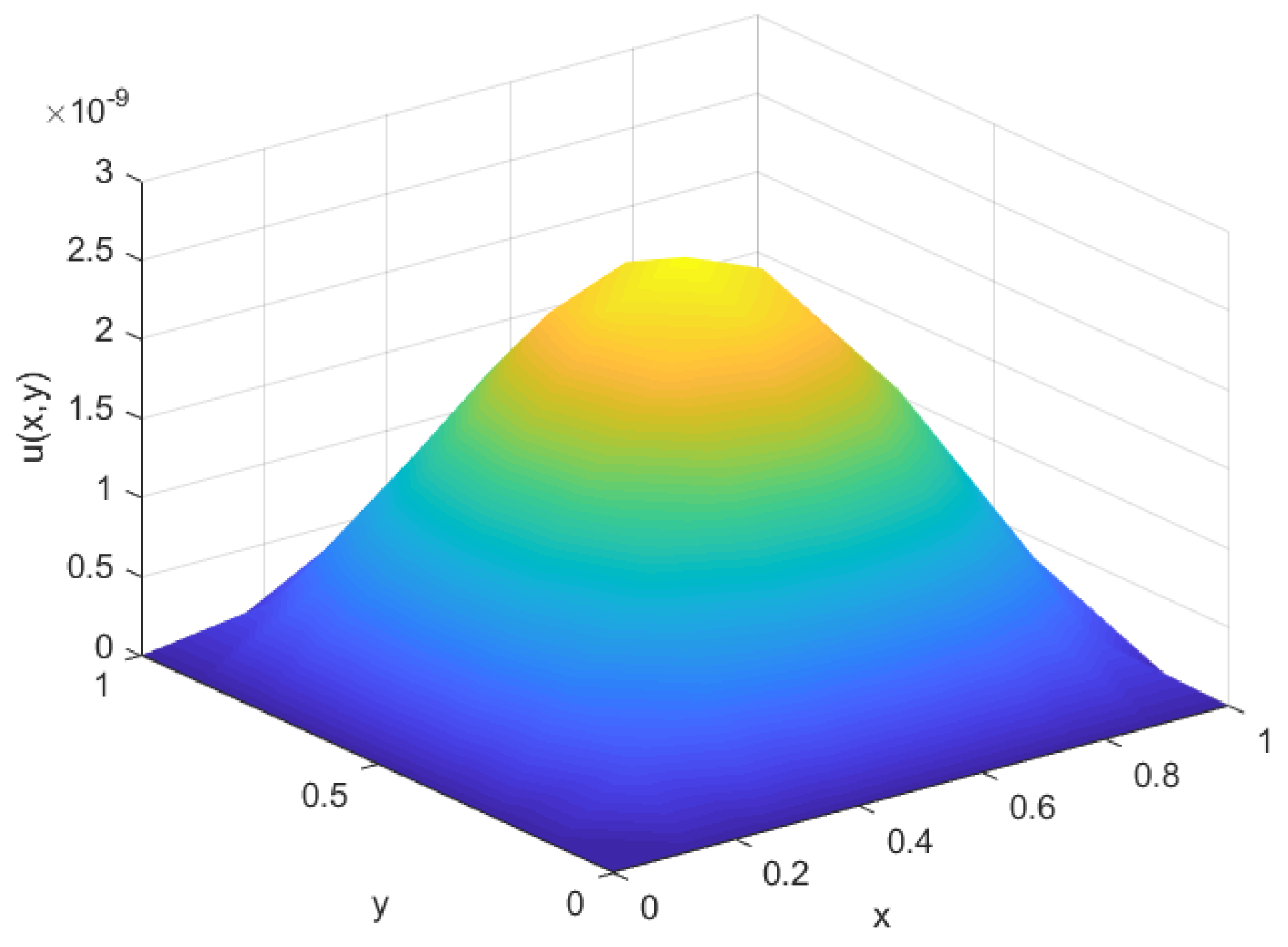
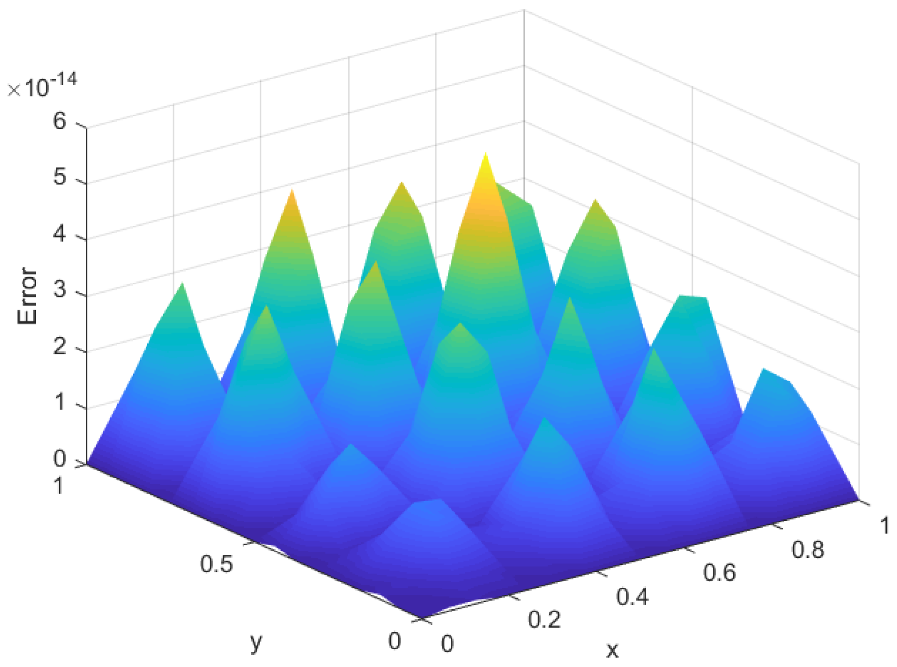
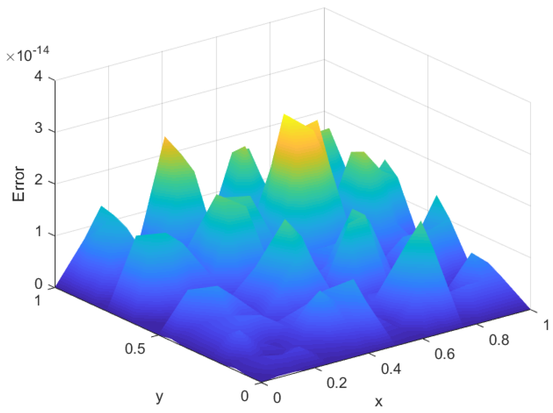
Figure 1, Figure 2, Figure 3 and Figure 4 show the spatiotemporal diagrams of the solution and error for the time step size $\tau ={\displaystyle \frac{1}{64}}$ and spatial step size $h={\displaystyle \frac{1}{8}}$.

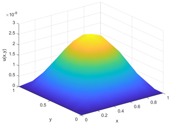
Figure 1. Numerical solution of FD scheme.

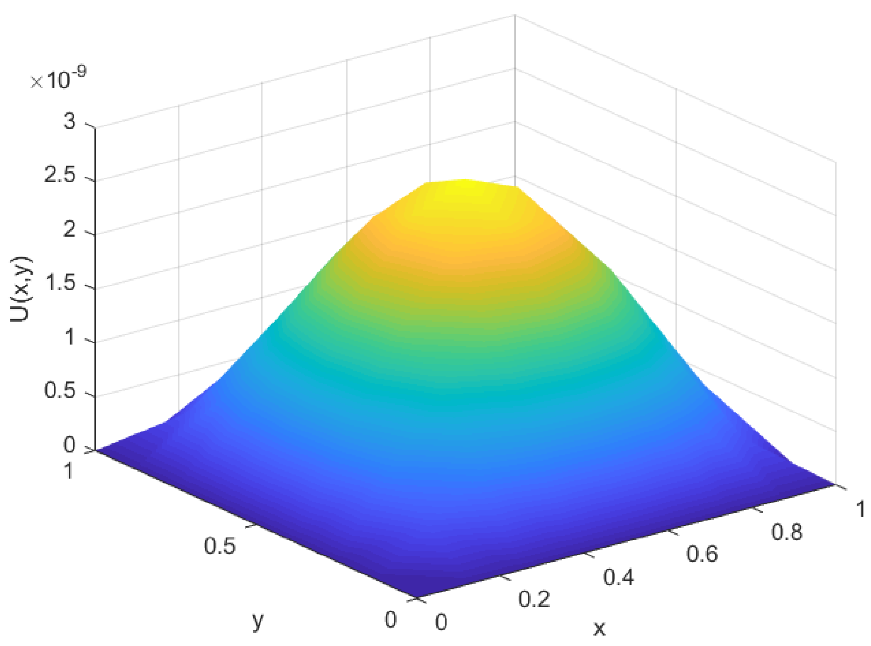
Figure 2. Dimensionality reduction solution.

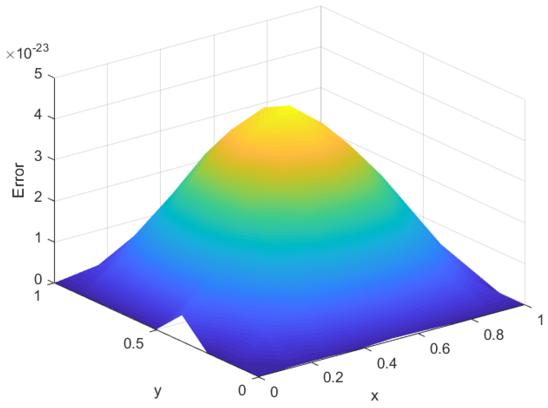
Figure 3. Numerical solution error of FD scheme.

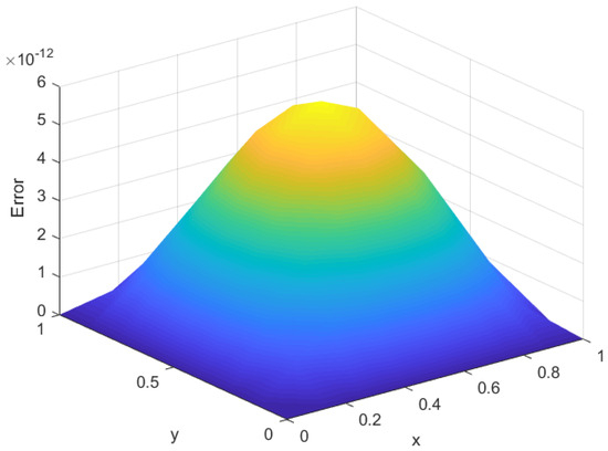
Figure 4. Dimensionality reduction solution error.

Figure 1 and Figure 2 show the spatiotemporal diagrams of the solutions obtained using the FD scheme and the POD reduced scheme, respectively. Figure 3 and Figure 4 show the spatiotemporal diagrams of the errors corresponding to the FD scheme and the POD reduced scheme, respectively. Figure 5 shows the error plot between the FD scheme and the old POD reduced scheme at time $T=1$ with the time step size $\tau ={\displaystyle \frac{1}{64}}$ and spatial step size $h={\displaystyle \frac{1}{8}}$. Figure 6 shows the error plot between the FD scheme and the new POD reduced scheme at time $T=1$ with the time step size $\tau ={\displaystyle \frac{1}{64}}$ and spatial step size $h={\displaystyle \frac{1}{8}}$. A comparison between Figure 5 and Figure 6 reveals that the FD scheme and the new POD reduced-order scheme exhibit smaller errors, demonstrating the superiority of the new POD reduced-order approach.

Figure 5. The error of the solution between two difference schemes.

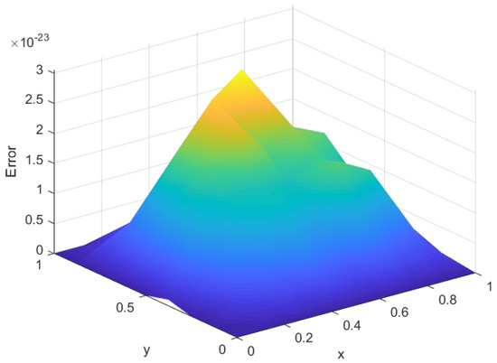
Figure 6. The error of the solution between two difference schemes.

The results clearly demonstrate that the new POD reduced-order scheme requires less CPU time than the old POD scheme. Furthermore, the new POD scheme exhibits smaller errors compared to the FD scheme. Both POD reduced-order schemes demand significantly less computational time than the compact finite-difference scheme. Since the POD method greatly reduces the degrees of freedom relative to the original difference scheme, computation time is substantially reduced, conclusively proving the superiority of the POD approach.

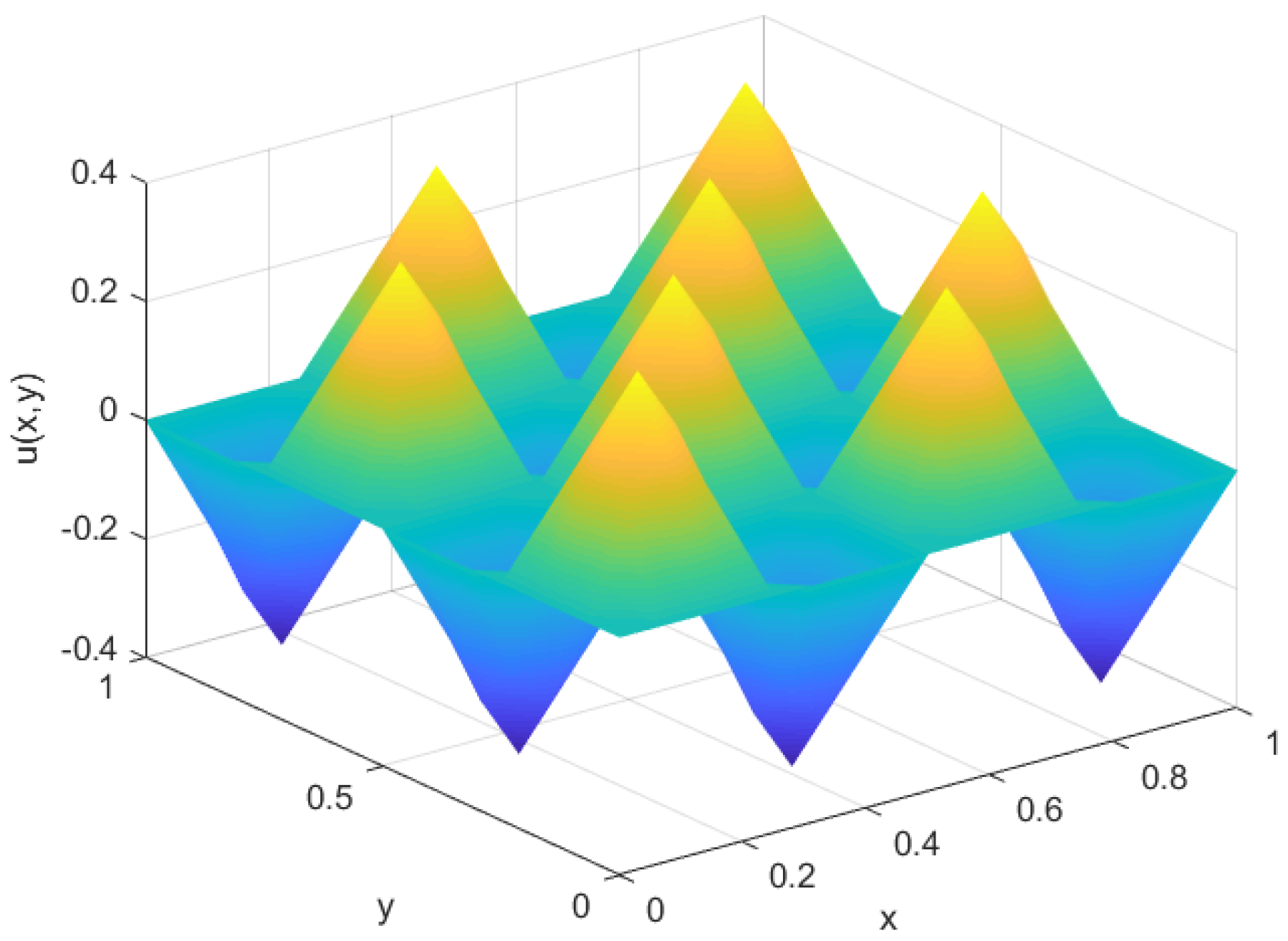
To validate the feasibility and generality of the proposed method, we conducted the following additional numerical experiments.

• Example 2

$$\left\{\begin{array}{c}{\displaystyle \frac{\partial u}{\partial t}}={\displaystyle \frac{1}{32{\pi }^2}}({\displaystyle \frac{{\partial }^{2}u}{\partial x^2}}+{\displaystyle \frac{{\partial }^{2}u}{\partial y^2}}),0<x,y<1,\hfill \\ u(x,y,0)=sin\left(4\pi x\right)sin\left(4\pi y\right),0<x,y<1,\hfill \\ u(0,y,t)=u(1,y,t)=0,t>0,\hfill \\ u(x,0,t)=u(x,1,t)=0,t>0.\hfill \end{array}\right.$$

The exact solution to this problem is

$$u(x,y,t)=e^{-t}sin\left(4\pi x\right)sin\left(4\pi y\right).$$

It can be seen from Table 7 and Table 8 that the POD reduced-order scheme achieves fourth-order convergence accuracy in the temporal and spatial dimensions.

Table 7. The $L_{\infty }$ error and convergence order of the POD reduced-order scheme when $\tau =h/4$, $T=1$.

h	$\mathit{\tau }$	Error (${\mathit{L}}_{\mathit{\infty }}$)	Rate
${\displaystyle \frac{1}{8}}$	${\displaystyle \frac{1}{32}}$	$1.0188\times {10}^{-2}$
${\displaystyle \frac{1}{16}}$	${\displaystyle \frac{1}{64}}$	$5.9735\times {10}^{-4}$	4.0922
${\displaystyle \frac{1}{32}}$	${\displaystyle \frac{1}{128}}$	$3.6676\times {10}^{-5}$	4.0257
${\displaystyle \frac{1}{64}}$	${\displaystyle \frac{1}{256}}$	$2.2818\times {10}^{-6}$	4.0066

Table 8. The $L_{\infty }$ error and convergence order of the POD reduced-order scheme when $\tau =1/1000$, $T=1$.

h	$\mathit{\tau }$	Error (${\mathit{L}}_{\mathit{\infty }}$)	Rate
${\displaystyle \frac{1}{8}}$	${\displaystyle \frac{1}{1000}}$	$1.0188\times {10}^{-2}$
${\displaystyle \frac{1}{16}}$	${\displaystyle \frac{1}{1000}}$	$5.9735\times {10}^{-4}$	4.0922
${\displaystyle \frac{1}{32}}$	${\displaystyle \frac{1}{1000}}$	$3.6676\times {10}^{-5}$	4.0257
${\displaystyle \frac{1}{64}}$	${\displaystyle \frac{1}{1000}}$	$2.2818\times {10}^{-6}$	4.0066

Table 9 and Table 10 show a comparison between the POD reduced-order scheme and the FD scheme in terms of CPU running time. It is apparent that the computational time (CPU time) for the POD reduced-order format is shorter than that of the compact finite-difference scheme. Moreover, when $\tau$ is smaller, the CPU time of the new POD scheme remains relatively brief.

Table 9. The CPU times of the FD scheme and the new POD reduced-order scheme when $\tau =h/4$, $T=1$.

h	$\mathit{\tau }$	FD Scheme(s)	New POD Scheme(s)
${\displaystyle \frac{1}{8}}$	${\displaystyle \frac{1}{32}}$	0.010216	0.0000535
${\displaystyle \frac{1}{16}}$	${\displaystyle \frac{1}{64}}$	0.06125	0.0007933
${\displaystyle \frac{1}{32}}$	${\displaystyle \frac{1}{128}}$	2.9724	0.0007105
${\displaystyle \frac{1}{64}}$	${\displaystyle \frac{1}{256}}$	194.2064	0.001047

Table 10. The CPU times of the FD scheme and the new POD reduced-order scheme when $\tau =h^2$, $T=1$.

h	$\mathit{\tau }$	FD Scheme(s)	New POD Scheme(s)
${\displaystyle \frac{1}{8}}$	${\displaystyle \frac{1}{64}}$	0.026935	0.060599
${\displaystyle \frac{1}{16}}$	${\displaystyle \frac{1}{256}}$	0.25121	0.0007229
${\displaystyle \frac{1}{32}}$	${\displaystyle \frac{1}{1024}}$	25.4047	0.0009537
${\displaystyle \frac{1}{64}}$	${\displaystyle \frac{1}{4096}}$	2638.6785	0.0014795

Table 11 shows the errors of the two POD schemes compared with the FD scheme. By examining this table, we can observe that the error between the new POD scheme and the FD scheme is smaller. This implies that the new POD scheme offers enhanced accuracy.

Table 11. The errors of the two POD schemes compared with the FD scheme when $\tau =h^2$, $T=1$.

h	$\mathit{\tau }$	Old POD Scheme	New POD Scheme
${\displaystyle \frac{1}{8}}$	${\displaystyle \frac{1}{64}}$	$2.3592\times {10}^{-14}$	$5.5511\times {10}^{-15}$
${\displaystyle \frac{1}{16}}$	${\displaystyle \frac{1}{256}}$	$3.2641\times {10}^{-14}$	$5.3013\times {10}^{-14}$
${\displaystyle \frac{1}{32}}$	${\displaystyle \frac{1}{1024}}$	$1.3878\times {10}^{-13}$	$9.6034\times {10}^{-14}$
${\displaystyle \frac{1}{64}}$	${\displaystyle \frac{1}{4096}}$	$6.4426\times {10}^{-13}$	$4.8311\times {10}^{-13}$

Figure 7, Figure 8, Figure 9 and Figure 10 show the spatiotemporal diagrams of the solution and error for the time step size $\tau ={\displaystyle \frac{1}{256}}$ and spatial step size $h={\displaystyle \frac{1}{16}}$.

Figure 7. Numerical solution of FD scheme.

Figure 8. Dimensionality reduction solution.

Figure 9. Numerical solution error of FD scheme.

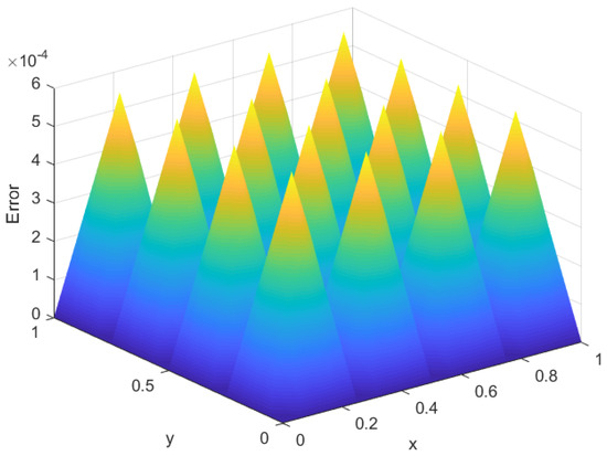
Figure 10. Dimensionality reduction solution error.

Figure 7 and Figure 8 show the spatiotemporal diagrams of the solutions obtained using the FD scheme and the POD reduced scheme, respectively. Figure 9 and Figure 10 show the spatiotemporal diagrams of the errors corresponding to the FD scheme and the POD reduced scheme, respectively. Figure 11 shows the error plot between the FD scheme and the old POD reduced scheme at time $T=1$ with the time step size $\tau ={\displaystyle \frac{1}{256}}$ and spatial step size $h={\displaystyle \frac{1}{16}}$. Figure 12 shows the error plot between the FD scheme and the new POD reduced scheme at time $T=1$ with the time step size $\tau ={\displaystyle \frac{1}{256}}$ and spatial step size $h={\displaystyle \frac{1}{16}}$. A comparison between Figure 11 and Figure 12 reveals that the FD scheme and the new POD reduced-order scheme exhibit smaller errors, demonstrating the superiority of the new POD reduced-order approach.

Figure 11. The error of the solution between two difference schemes.

Figure 12. The error of the solution between two difference schemes.

The results clearly demonstrate that the new POD reduced-order scheme requires less CPU time than the old POD scheme. Furthermore, the new POD scheme exhibits smaller errors compared to the FD scheme. Both POD reduced-order schemes demand significantly less computational time than the compact finite-difference scheme. Since the POD method greatly reduces the degrees of freedom relative to the original difference scheme, computation time is substantially reduced-conclusively proving the superiority of the POD approach.

6. Conclusions

In this paper, we first propose a high-accuracy FD scheme for two-dimensional diffusion equations. Spatial variables are discretized using fourth-order spline functions, and the $(2,2)$ Padé approximation is used for the time-derivative, then converted into matrix form. Next, the POD method and cumulative contribution rate are applied to optimize and reduce the order of the scheme. A reduced-order algorithm based on POD for compact finite difference is developed, along with error estimates. Numerical simulations verify the analysis, and comparisons are made between the two POD schemes and the original FD scheme. Results demonstrate that the new POD scheme is more efficient, maintains sufficient accuracy, diminishes the degrees of freedom, enhances computational efficiency, and decreases CPU time. This new POD-based order-reduction method is promising for solving 3D and higher-dimensional complex PDEs.

Finally, due to the length limitations of this paper, the impact of changes in the discretization parameters discussed herein will be further explored in future research. This method investigates ordinary two-dimensional linear parabolic equations, and in subsequent studies, we can extend it to nonlinear parabolic problems and higher-dimensional parabolic problems. Additionally, since the approach in this paper is tens of thousands of times faster than traditional difference schemes when handling fine grids, we can compare it with other established dimension reduction techniques, such as dynamic mode decomposition (DMD), to comprehensively understand the relative performance and advantages of this method. In practical applications, the POD method, although capable of significantly reducing the computational dimension of diffusion equations, still encounters multiple challenges. Its linear nature makes it difficult to capture strong nonlocal or nonlinear dynamics. The number, distribution, and parameter sensitivity of snapshots directly determine the accuracy of dimensionality reduction. The treatment of boundary conditions and time-varying coefficients requires additional skills. Issues such as storage and SVD computational bottlenecks caused by high-dimensional snapshots and the failure of parameter extrapolation cannot be ignored. To address these challenges, strategies such as adaptive snapshots, local POD, nonlinear dimensionality reduction (e.g., POD-DNN coupling), or parametric POD can be employed to mitigate theoretical limitations and enhance engineering robustness.

References

- Lin, Y.; Gao, X.; Xiao, M. A high-order finite difference method for 1D nonhomogeneous heat equations. Numer. Methods Partial Differ. Equ. 2009, 25, 327–346. [Google Scholar] [CrossRef]
- Zhao, J.; Dai, W.; Niu, T. Fourth-order compact schemes of a heat conduction problem with Neumann boundary conditions. Numer. Methods Partial Diff. Equ. 2007, 23, 949–959. [Google Scholar] [CrossRef]
- Gao, F.; Chi, C. Unconditionally stable difference schemes for a one-space-dimensional linear hyperbolic equation. Appl. Math. Comput. 2006, 187, 1272–1276. [Google Scholar] [CrossRef]
- Liu, H.; Liu, L.; Chen, Y. A semi-discretization method based on quartic splines for solving one-space-dimensional hyperbolic equations. Appl. Math. Comput. 2009, 210, 508–514. [Google Scholar] [CrossRef]
- Zhang, Y. [3, 3] Padé approximation method for solving space fractional Fokker–Planck equations. Appl. Math. Lett. 2014, 35, 109–114. [Google Scholar] [CrossRef]
- Chen, J.; Ge, Y. High order locally one-dimensional methods for solving two-dimensional parabolic equations. Adv. Differ. Equ. 2018, 2018, 361. [Google Scholar] [CrossRef]
- Holmes, P.; Lumley, J.L.; Berkooz, G. Turbulence, Coherent Structures, Dynamical Systems and Symmetry, 2nd ed.; Cambridge University Press: Cambridge, UK, 2012. [Google Scholar]
- Luo, Z.D.; Chen, G. Proper Orthogonal Decomposition Methods for Partial Differential Equations; Academic Press of Elsevier: San Diego, VA, USA, 2018. [Google Scholar]
- Volkwein, S. Proper Orthogonal Decomposition: Applications in Optimization and Control. 2007. Available online: http://www.math.uni-konstanz.de/numerik/personen/volkwein/teaching/Lecture-Notes-Volkwein.pdf (accessed on 15 June 2025).
- Sirovich, L. Turbulence and the dynamics of coherent structures. Part I: Coherent structures. Q. Appl. Math. 1987, XLV, 561–571. [Google Scholar] [CrossRef]
- Sirovich, L. Turbulence and the dynamics of coherent structures. Part III: Dynamics and scaling. Q. Appl. Math. 1987, XLV, 583–590. [Google Scholar] [CrossRef]
- Selten, F.M. Baroclinic empirical orthogonal functions as basis functions in an atmospheric model. J. Atmos. Sci. 1997, 54, 2099–2114. [Google Scholar] [CrossRef]
- Crommelin, D.T.; Majda, A.J. Strategies for Model Reduction: Comparing Different Optimal Bases. J. Atmos. Sci. 2004, 61, 2206–2217. [Google Scholar] [CrossRef]
- Sun, P.; Luo, Z.; Zhou, Y. Some reduced finite difference schemes based on a proper orthogonal decomposition technique for parabolic equations. Appl. Numer. Math. 2009, 60, 154–164. [Google Scholar] [CrossRef]
- Di, Z.; Luo, Z.; Xie, Z.; Wang, A.; Navon, I.M. An optimizing implicit difference scheme based on proper orthogonal decomposition for the two-dimensional unsaturated soil water flow equation. Int. J. Numer. Methods Fluids 2012, 68, 1324–1340. [Google Scholar] [CrossRef]
- Luo, Z.; Teng, F.; Di, Z. A POD-based reduced-order finite difference extrapolating model with fully second-order accuracy for non-stationary Stokes equations. Int. J. Comput. Fluid Dyn. 2014, 28, 428–436. [Google Scholar] [CrossRef]
- Xia, H.; Luo, Z. An optimized finite difference Crank–Nicolson iterative scheme for the 2D Sobolev equation. Adv. Differ. Equ. 2017, 2017, 196. [Google Scholar] [CrossRef]
- Deng, Q.; Luo, Z. A reduced-order extrapolated finite difference iterative scheme for uniform transmission line equation. Appl. Numer. Math. 2022, 172, 514–524. [Google Scholar] [CrossRef]
- Ren, X.; Li, H. A Reduced-Dimension Weighted Explicit Finite Difference Method Based on the Proper Orthogonal Decomposition Technique for the Space-Fractional Diffusion Equation. Axioms 2024, 1, 461. [Google Scholar] [CrossRef]
- Li, H.; Luo, Z.; Gao, J. A New Reduced-Order fve Algorithm Based on POD Method for Viscoelastic Equations. Acta Math. Sci. 2013, 33, 1076–1098. [Google Scholar] [CrossRef]
- Luo, Z.; Du, J.; Xie, Z.; Guo, Y. A reduced stabilized mixed finite element formulation based on proper orthogonal decomposition for the non-stationary Navier–Stokes equations. Int. J. Numer. Methods Eng. 2011, 88, 31–46. [Google Scholar] [CrossRef]
- Li, Y.; Luo, Z.; Liu, C. The Mixed Finite Element Reduced-Dimension Technique with Unchanged Basis Functions for Hydrodynamic Equation. Mathematics 2023, 11, 807. [Google Scholar] [CrossRef]
- Luo, Z.; Yang, J. The reduced-order method of continuous space-time finite element scheme for the non-stationary incompressible flows. J. Comput. Physics 2022, 456, 111044. [Google Scholar] [CrossRef]
- Yang, J.; Luo, Z.D. A reduced-order extrapolating space-time continuous finite element method for the 2D Sobolev equation. Numer. Methods Partial Differ. Equ. 2020, 36, 1446–1459. [Google Scholar] [CrossRef]
- Luo, Z.D.; Jin, S.J. A reduced-order extrapolated Crank–Nicolson collocation spectral method based on proper orthogonal decomposition for the two-dimensional viscoelastic wave equations. Numer. Methods Partial Differ. Equ. 2020, 36, 49–65. [Google Scholar] [CrossRef]
- Luo, Z.D.; Jiang, W. A reduced-order extrapolated Crank–Nicolson finite spectral element method for the 2D non-stationary Navier–Stokes equations about vorticity-stream functions. Appl. Numer. Math. 2020, 147, 161–173. [Google Scholar] [CrossRef]
Disclaimer/Publisher’s Note: The statements, opinions and data contained in all publications are solely those of the individual author(s) and contributor(s) and not of MDPI and/or the editor(s). MDPI and/or the editor(s) disclaim responsibility for any injury to people or property resulting from any ideas, methods, instructions or products referred to in the content. |
© 2025 by the authors. Licensee MDPI, Basel, Switzerland. This article is an open access article distributed under the terms and conditions of the Creative Commons Attribution (CC BY) license (https://creativecommons.org/licenses/by/4.0/).