
Unmanned Aerial Vehicle Position Tracking Using Nonlinear Autoregressive Exogenous Networks Learned from Proportional-Derivative Model-Based Guidance


Abstract
1. Introduction
2. State of the Art
3. Methodology
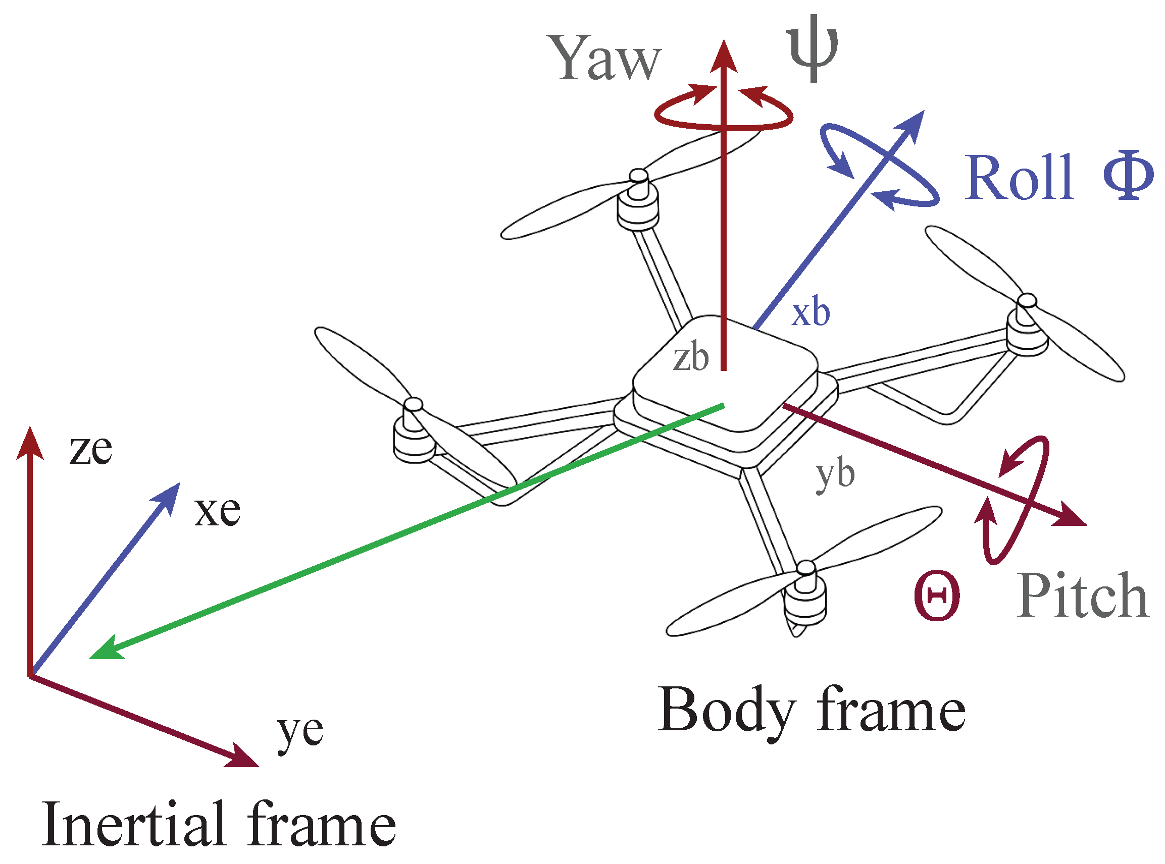
3.1. Mathematical Model of a Quadcopter
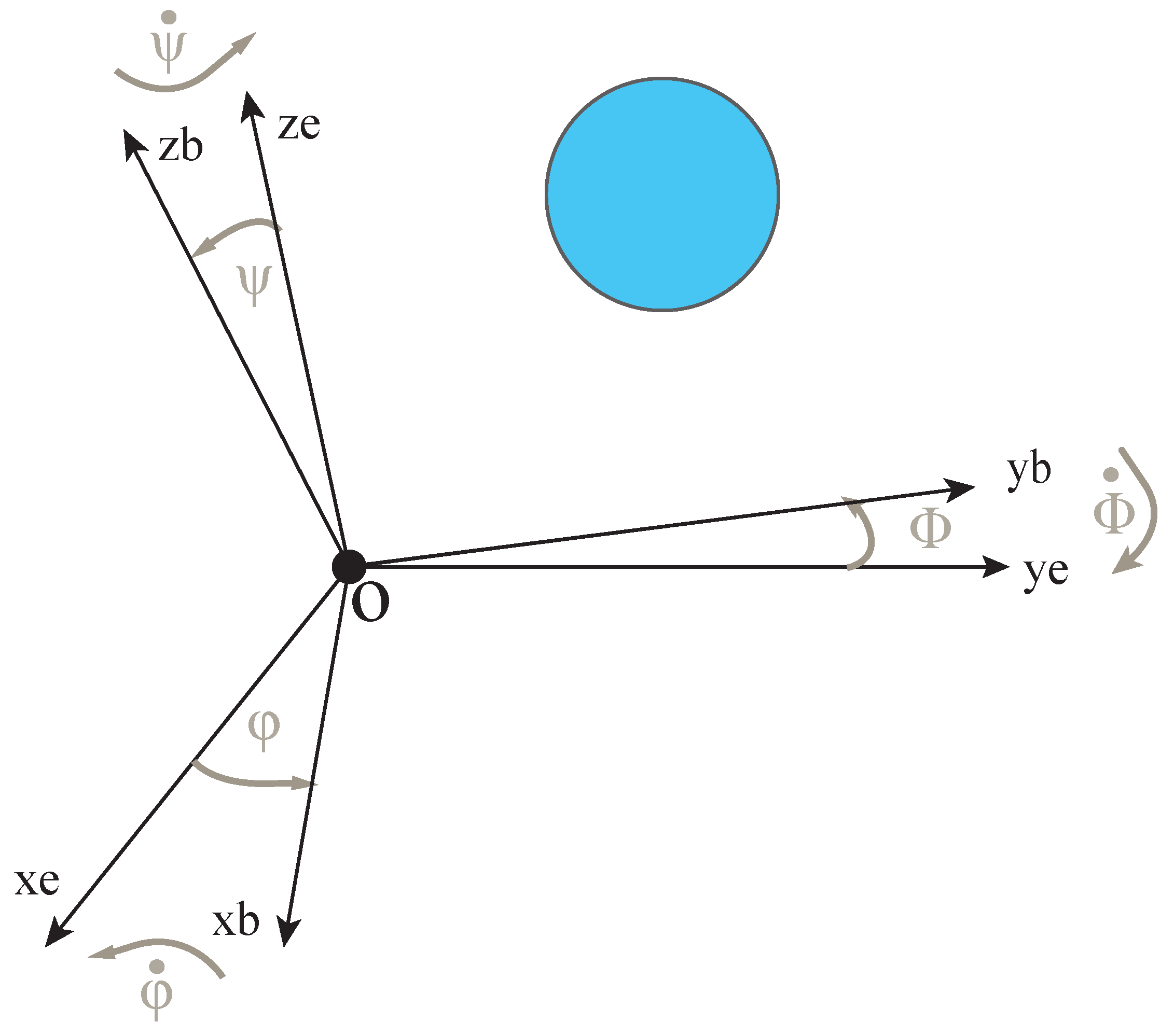
3.2. Coordinate Transformation Between Reference Frames
3.3. Kinematic and Dynamic Modeling of Translational and Rotational Motion
3.4. Linearization Around Hover and Decoupled Subsystem Modeling
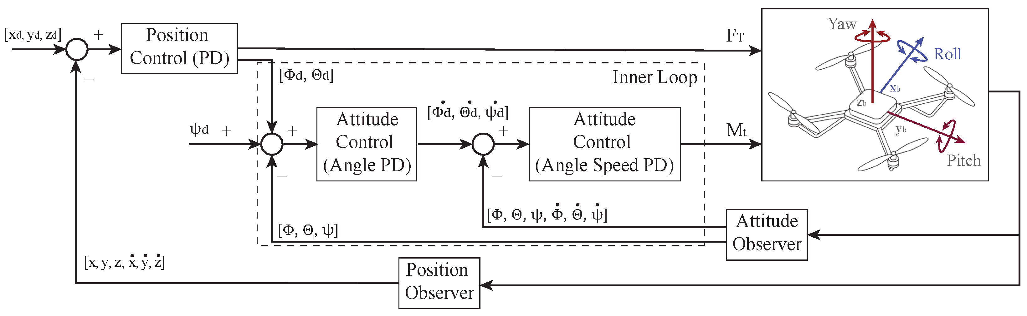
3.5. Cascaded Control Architecture and PD-Based Stabilization Strategy
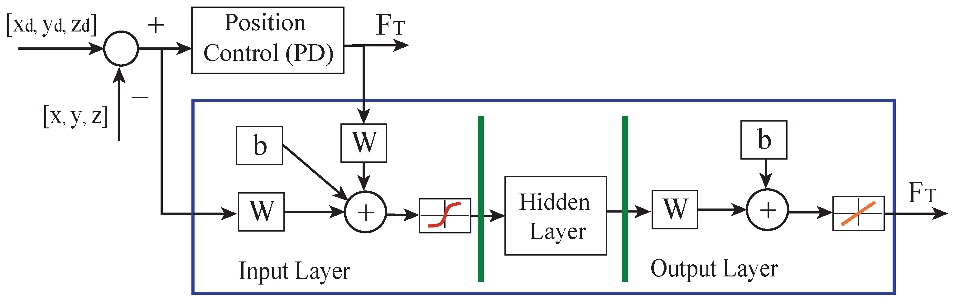
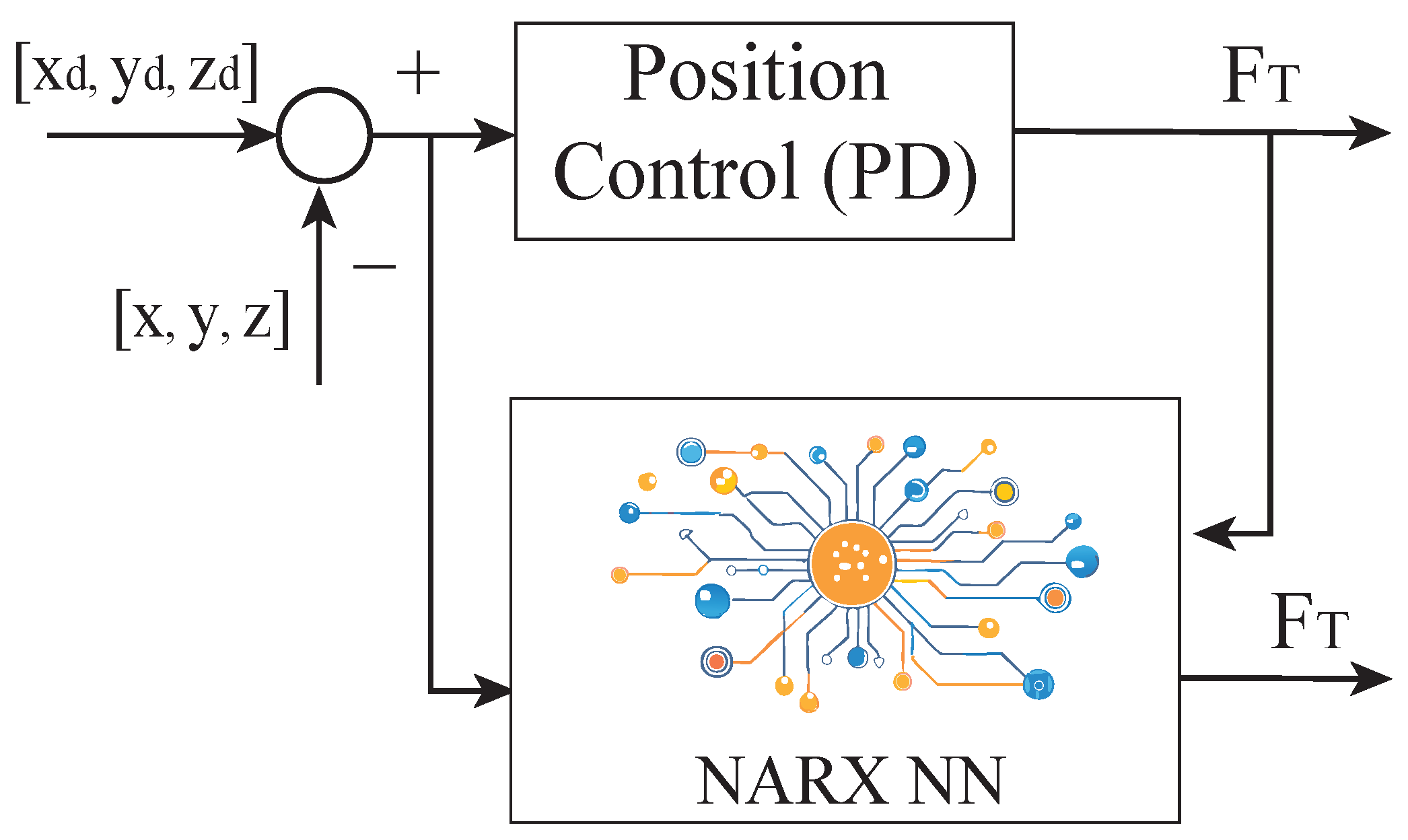
3.6. NARX Controller Design and Implementation Details
3.7. Optimization Problem for Trajectory Tracking
4. Results and Discussion
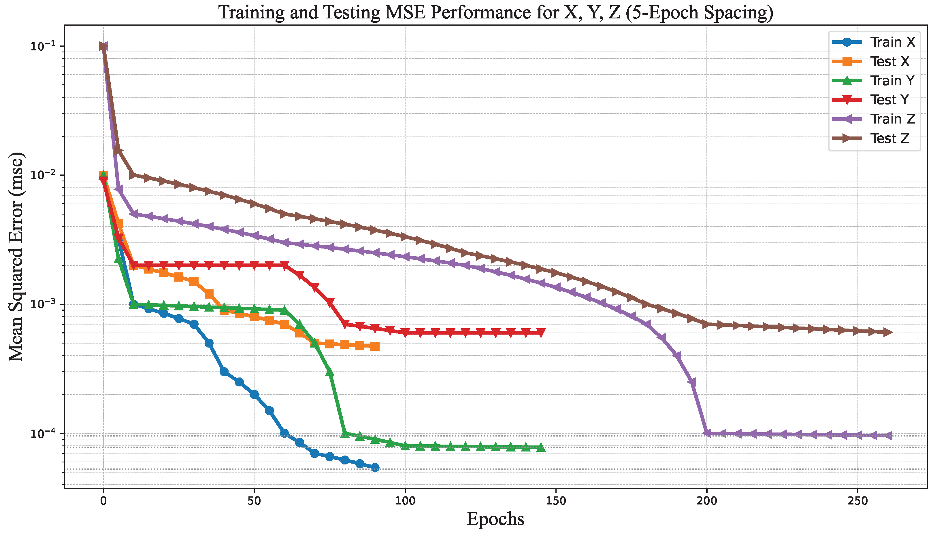
4.1. Training Evaluation and Axis-Wise Performance of the NARX Controllers
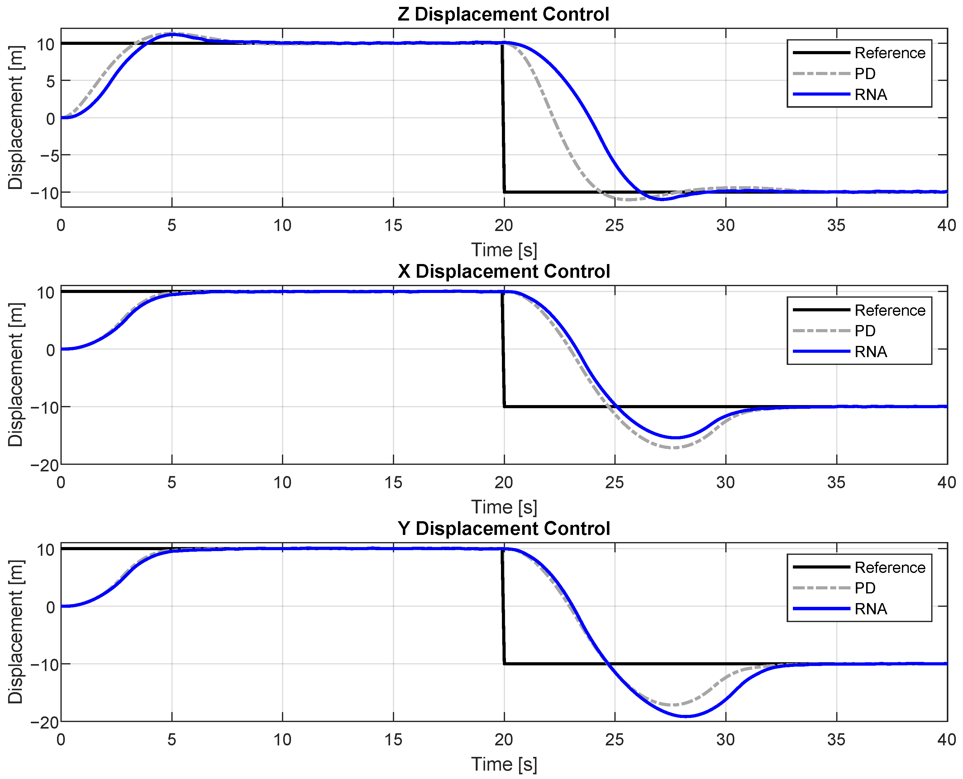
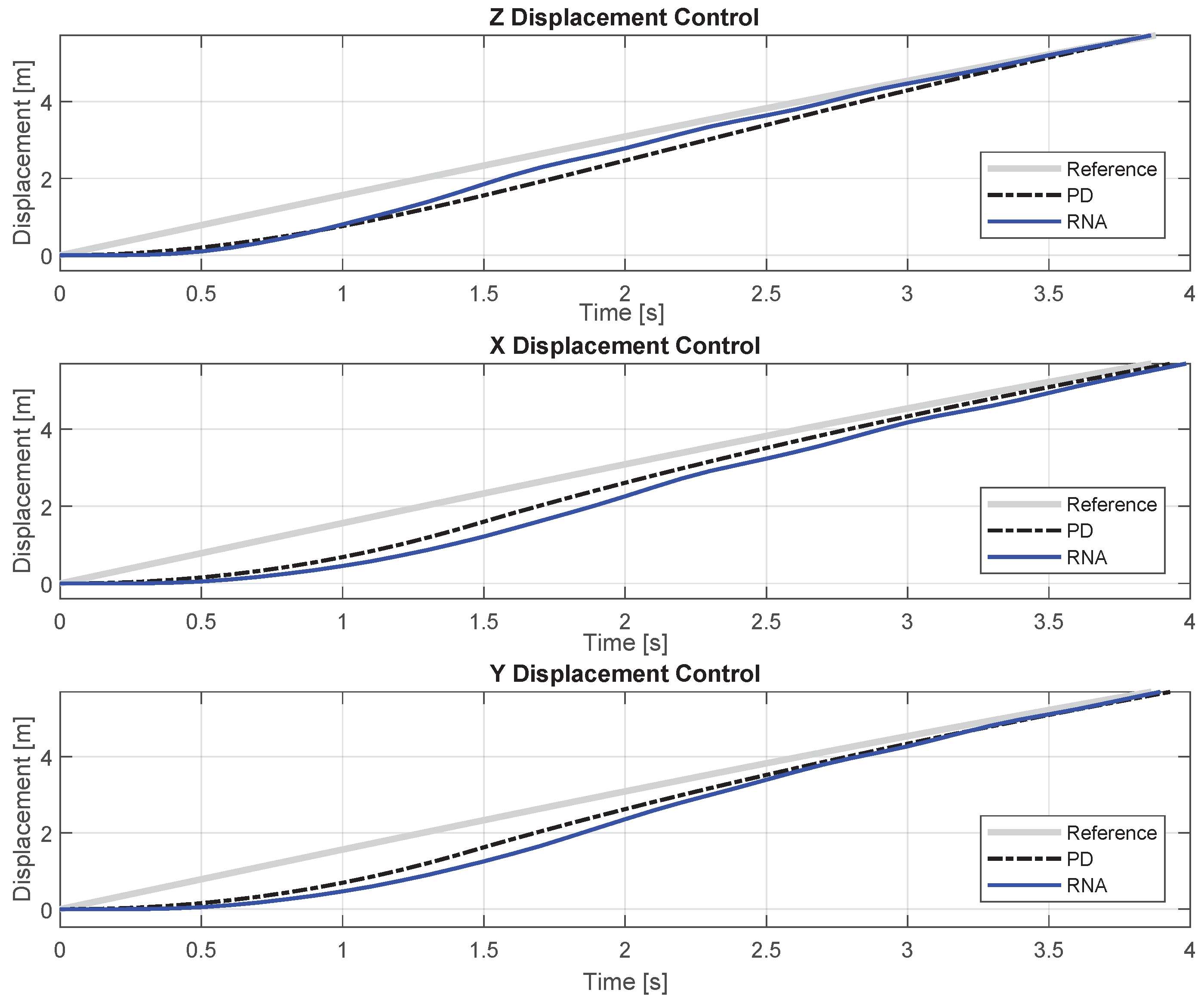
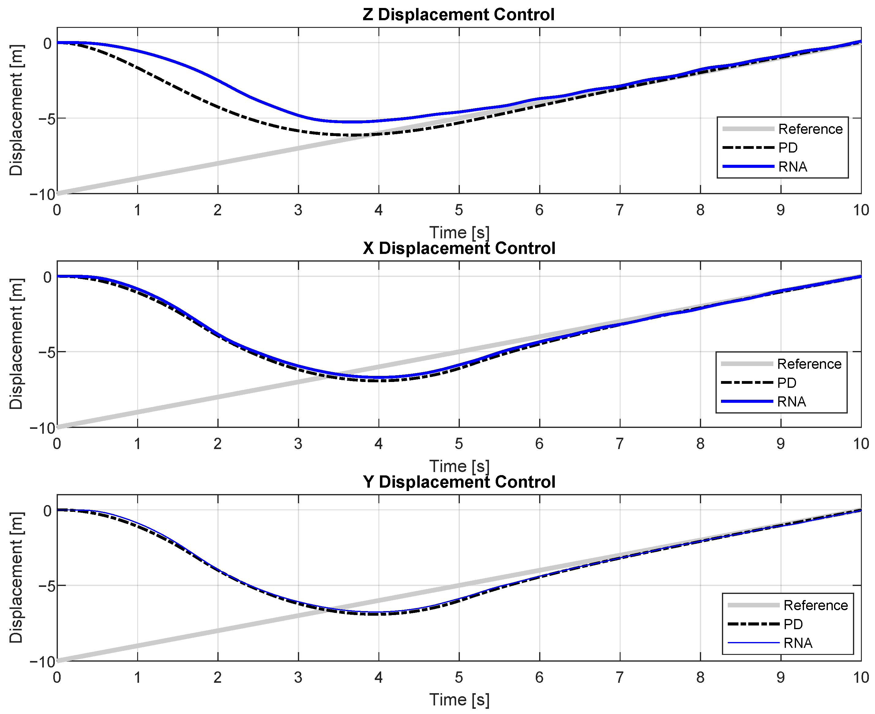
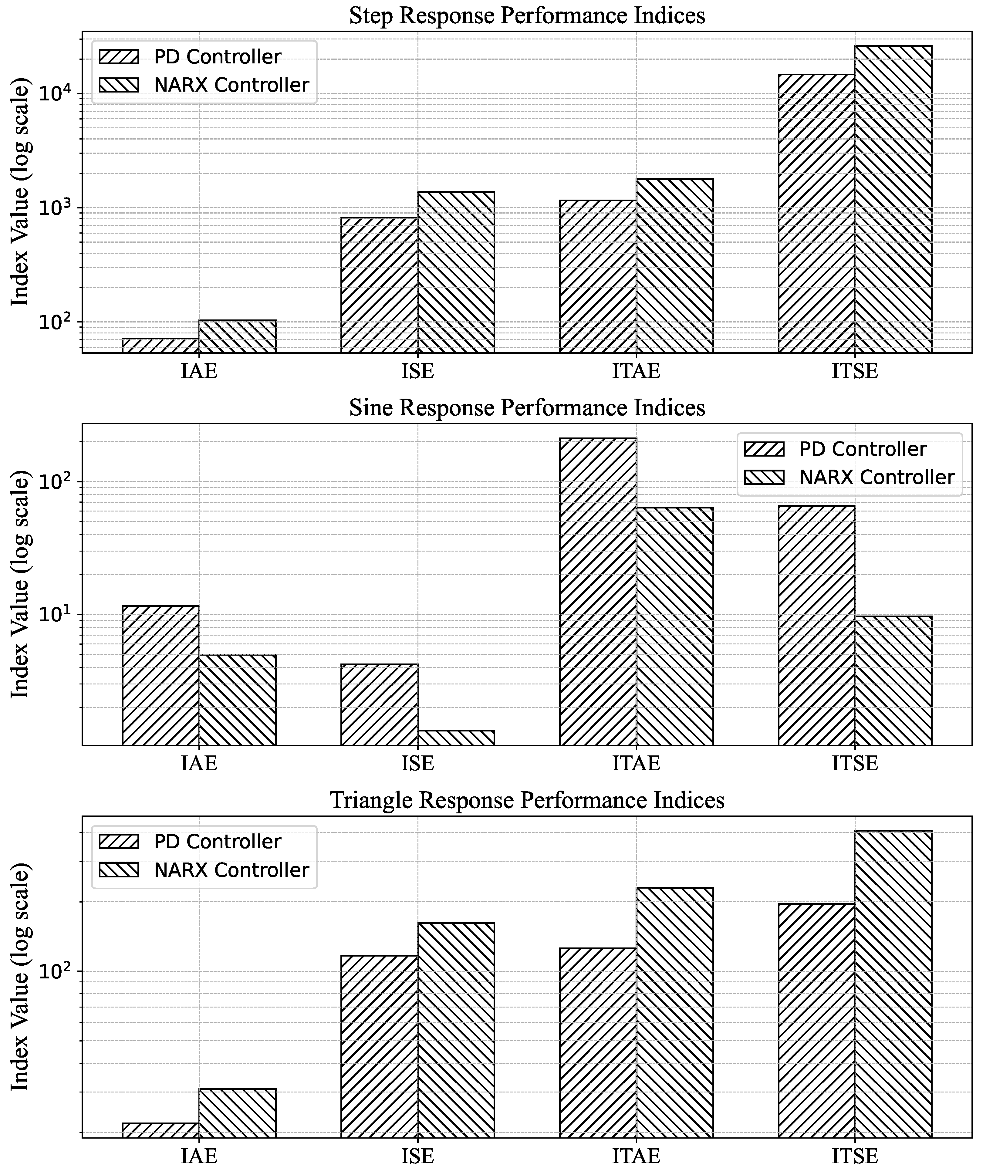
4.2. Trajectory Tracking Performance Under Diverse Reference Inputs
5. Conclusions and Future Works
Author Contributions
Funding
Data Availability Statement
Acknowledgments
Conflicts of Interest
Nomenclature
| Symbol | Description |
| Position in inertial frame (Earth-fixed). | |
| Position in body frame (UAV-fixed). | |
| Linear velocities in body frame. | |
| Linear velocities in inertial frame. | |
| Roll, pitch, and yaw angles (Euler angles). | |
| Time derivatives of Euler angles. | |
| Roll, pitch, and yaw angular velocity of the body frame (Euler angle rates). | |
| Rotation matrices for each axis (roll, pitch, yaw). | |
| Full rotation matrix from body to inertial frame. | |
| Transformation matrix and its inverse for angular velocity conversion. | |
| I | Inertia matrix of the UAV. |
| Principal moments of inertia. | |
| Torques about roll, pitch, and yaw axes. | |
| M | Torque vector. |
| w | Angular velocity vector . |
| m | Mass of the quadcopter. |
| g | Gravitational acceleration. |
| Total thrust generated by the UAV. | |
| Thrust from rotor i, . | |
| Thrust coefficient for rotor i. | |
| l | Distance from UAV center to motor (arm length). |
| d | Drag coefficient of the rotors. |
| Desired position in inertial frame. | |
| Desired yaw angle. | |
| Desired roll and pitch angles. | |
| Commanded total thrust. | |
| Commanded yaw rate. | |
| Transfer function of PD controller. | |
| Proportional gain and derivative time constant. | |
| Tracking error between reference and actual output. | |
| Desired (reference) signal and actual output. | |
| State and control input vectors. | |
| UAV nonlinear dynamics function. | |
| Lower and upper bounds for control inputs. | |
| State constraints for position, velocity, and angles. | |
| J | Objective function for trajectory tracking. |
| MSE | Mean Squared Error metric. |
| Coefficient of determination for model fit. | |
| IAE | Integral of the Absolute Error; measures total accumulated error over time. |
| ISE | Integral of the Squared Error; penalizes larger errors more heavily. |
| ITAE | Integral of Time-weighted Absolute Error; emphasizes errors that persist over time. |
| ITSE | Integral of Time-weighted Squared Error; highlights sustained large errors. |
References
- Yoon, J.; Doh, J. Optimal PID Control for Hovering Stabilization of Quadcopter Using Long Short Term Memory. Adv. Eng. Inform. 2022, 53, 101679. [Google Scholar] [CrossRef]
- Jiang, F.; Pourpanah, F.; Hao, Q. Design, Implementation, and Evaluation of a Neural-Network-Based Quadcopter UAV System. IEEE Trans. Ind. Electron. 2020, 67, 2076–2085. [Google Scholar] [CrossRef]
- Pinzón, S.; Pavón, W. Diseño de Sistemas de Control Basados en el Análisis del Dominio en Frecuencia. Rev. Técnica Energía 2019, 15, 76–82. [Google Scholar] [CrossRef]
- Wu, Z.; Ye, J.; Song, T. Dynamic Event-Triggered Prescribed Performance Robust Control for Aggressive Quadrotor Flight. Aerospace 2024, 11, 301. [Google Scholar] [CrossRef]
- Hadid, S.; Boushaki, R.; Boumchedda, F.; Merad, S. Enhancing Quadcopter Autonomy: Implementing Advanced Control Strategies and Intelligent Trajectory Planning. Automation 2024, 5, 151–175. [Google Scholar] [CrossRef]
- Dougherty, S.; Oo, N.L.; Zhao, D. Effects of propeller separation and onset flow condition on the performance of quadcopter propellers. Aerosp. Sci. Technol. 2024, 145, 108837. [Google Scholar] [CrossRef]
- Yih, C.-C.; Wu, S.-J. Sliding Mode Path Following and Control Allocation of a Tilt-Rotor Quadcopter. Appl. Sci. 2022, 12, 11088. [Google Scholar] [CrossRef]
- Yao, W.-S.; Lin, C.-Y. Dynamic Stiffness Enhancement of the Quadcopter Control System. Electronics 2022, 11, 2206. [Google Scholar] [CrossRef]
- Lu, P.; Liu, M.; Zhang, X.; Zhu, G.; Li, Z.; Su, C.-Y. Neural Network Based Adaptive Event-Triggered Control for Quadrotor Unmanned Aircraft Robotics. Machines 2022, 10, 617. [Google Scholar] [CrossRef]
- Sheta, A.; Braik, M.; Maddi, D.R.; Mahdy, A.; Aljahdali, S.; Turabieh, H. Optimization of PID Controller to Stabilize Quadcopter Movements Using Meta-Heuristic Search Algorithms. Appl. Sci. 2021, 11, 6492. [Google Scholar] [CrossRef]
- Nguyen, A.T.; Xuan-Mung, N.; Hong, S.-K. Quadcopter Adaptive Trajectory Tracking Control: A New Approach via Backstepping Technique. Appl. Sci. 2019, 9, 3873. [Google Scholar] [CrossRef]
- Bari, S.; Zehra Hamdani, S.S.; Khan, H.U.; Rehman, M.U.; Khan, H. Artificial Neural Network Based Self-Tuned PID Controller for Flight Control of Quadcopter. In Proceedings of the 2019 International Conference on Engineering and Emerging Technologies, ICEET 2019, Lahore, Pakistan, 21–22 February 2019; pp. 1–5. [Google Scholar] [CrossRef]
- Olaz, X.; Alaez, D.; Prieto, M.; Villadangos, J.; Astrain, J.J. Quadcopter neural controller for take-off and landing in windy environments. Expert Syst. Appl. 2023, 225, 120146. [Google Scholar] [CrossRef]
- Maaruf, M.; Abubakar, A.N.; Gulzar, M.M. Adaptive Backstepping and Sliding Mode Control of a Quadrotor. J. Braz. Soc. Mech. Sci. Eng. 2024, 46, 630. [Google Scholar] [CrossRef]
- Nobahari, H.; Sharifi, A. Multiple model extended continuous ant colony filter applied to real-time wind estimation in a fixed-wing UAV. Eng. Appl. Artif. Intell. 2020, 92, 103629. [Google Scholar] [CrossRef]
- Sopov, E. Solving a Problem of the Lateral Dynamics Identification of a UAV using a Hyper-heuristic for Non-stationary Optimization. In Proceedings of the 13th International Joint Conference on Computational Intelligence (IJCCI 2021), Online Streaming, 25–27 October 2021; pp. 107–114. [Google Scholar] [CrossRef]
- Maaruf, M.; Hamanah, W.M.; Abido, M.A. Hybrid Backstepping Control of a Quadrotor Using a Radial Basis Function Neural Network. Mathematics 2023, 11, 991. [Google Scholar] [CrossRef]
- Filimonov, A.B.; Filimonov, N.B.; Pham, Q.P. Planning of Drones Flight of Routes when Group Patrolling of Large Extended Territories. In Proceedings of the 2023 V International Conference on Control in Technical Systems (CTS), Saint Petersburg, Russia, 21–23 September 2023; pp. 228–231. [Google Scholar] [CrossRef]
- Venturini, F.; Mason, F.; Pase, F.; Chiariotti, F.; Testolin, A.; Zanella, A.; Zorzi, M. Distributed Reinforcement Learning for Flexible and Efficient UAV Swarm Control. IEEE Trans. Cogn. Commun. Netw. 2021, 7, 955–969. [Google Scholar] [CrossRef]
- Lyu, Z.; Zhu, G.; Xu, J. Joint Maneuver and Beamforming Design for UAV-Enabled Integrated Sensing and Communication. IEEE Trans. Wirel. Commun. 2023, 22, 2424–2440. [Google Scholar] [CrossRef]
- Mahmoud, M.S.; Maaruf, M. Robust Adaptive Multilevel Control of a Quadrotor. IEEE Access 2020, 8, 167684–167692. [Google Scholar] [CrossRef]
- Li, L.; Chang, T.-H.; Cai, S. UAV Positioning and Power Control for Two-Way Wireless Relaying. IEEE Trans. Wirel. Commun. 2020, 19, 1008–1024. [Google Scholar] [CrossRef]
- Dorling, K.; Heinrichs, J.; Messier, G.G.; Magierowski, S. Vehicle Routing Problems for Drone Delivery. IEEE Trans. Syst. Man Cybern. Syst. 2017, 47, 70–85. [Google Scholar] [CrossRef]
- Goerzen, C.; Kong, Z.; Mettler, B. A Survey of Motion Planning Algorithms from the Perspective of Autonomous UAV Guidance. J. Intell. Robot. Syst. 2010, 57, 65–100. [Google Scholar] [CrossRef]
- Nikolos, I.K.; Valavanis, K.P.; Tsourveloudis, N.C.; Kostaras, A.N. Evolutionary algorithm based offline/online path planner for UAV navigation. IEEE Trans. Syst. Man, Cybern. Part (Cybern.) 2003, 33, 898–912. [Google Scholar] [CrossRef]
- Mofid, O.; Mobayen, S. Adaptive sliding mode control for finite-time stability of quad-rotor UAVs with parametric uncertainties. ISA Trans. 2018, 72, 1–14. [Google Scholar] [CrossRef]
- Zhao, H.; Wang, H.; Wu, W.; Wei, J. Deployment Algorithms for UAV Airborne Networks Toward On-Demand Coverage. IEEE J. Sel. Areas Commun. 2018, 36, 2015–2031. [Google Scholar] [CrossRef]
- Fadlullah, Z.M.; Takaishi, D.; Nishiyama, H.; Kato, N.; Miura, R. A dynamic trajectory control algorithm for improving the communication throughput and delay in UAV-aided networks. IEEE Netw. 2016, 30, 100–105. [Google Scholar] [CrossRef]
- Radmanesh, M.; Kumar, M.; Guentert, P.H.; Sarim, M. Overview of Path-Planning and Obstacle Avoidance Algorithms for UAVs: A Comparative Study. Unmanned Syst. 2018, 06, 95–118. [Google Scholar] [CrossRef]
- Faiçal, B.S.; Freitas, H.; Gomes, P.H.; Mano, L.Y.; Pessin, G.; de Carvalho, A.C.P.L.F.; Krishnamachari, B.; Ueyama, J. An adaptive approach for UAV-based pesticide spraying in dynamic environments. Comput. Electron. Agric. 2017, 138, 210–223. [Google Scholar] [CrossRef]
- Altan, A. Performance of Metaheuristic Optimization Algorithms based on Swarm Intelligence in Attitude and Altitude Control of Unmanned Aerial Vehicle for Path Following. In Proceedings of the 2020 4th International Symposium on Multidisciplinary Studies and Innovative Technologies (ISMSIT), Istanbul, Turkey, 22–24 October 2020; pp. 1–6. [Google Scholar] [CrossRef]
- Shetty, V.K.; Sudit, M.; Nagi, R. Priority-based assignment and routing of a fleet of unmanned combat aerial vehicles. Comput. Oper. Res. 2008, 35, 1813–1828. [Google Scholar] [CrossRef]
- Yaman, O.; Yol, F.; Altinors, A. A Fault Detection Method Based on Embedded Feature Extraction and SVM Classification for UAV Motors. Microprocess. Microsyst. 2022, 94, 104683. [Google Scholar] [CrossRef]
- Labbadi, M.; Cherkaoui, M. Robust adaptive backstepping fast terminal sliding mode controller for uncertain quadrotor UAV. Aerosp. Sci. Technol. 2019, 93, 105306. [Google Scholar] [CrossRef]
- Pazmiño, R.; Pavon, W.; Armstrong, M.; Simani, S. Performance Evaluation of Fractional Proportional–Integral–Derivative Controllers Tuned by Heuristic Algorithms for Nonlinear Interconnected Tanks. Algorithms 2024, 17, 306. [Google Scholar] [CrossRef]
- Salazar, D.; Pavón, W.; Montalvo, W.; Zambrano, J.C. Heuristic Tuning and Decoupling Strategies for Multivariable Systems: An Integrated TIA Portal and Matlab-Simulink Approach. In Proceedings of the International Conference on Science, Technology and Innovation for Society, Guayaquil, Ecuador, 23–24 October 2024; Springer: Berlin/Heidelberg, Germany, 2024; pp. 395–405. [Google Scholar] [CrossRef]
- Islam, S.; Liu, P.X.; El Saddik, A. Nonlinear adaptive control for quadrotor flying vehicle. Nonlinear Dyn. 2014, 78, 117–133. [Google Scholar] [CrossRef]
- Santoso, F.; Garratt, M.A.; Anavatti, S.G. Hybrid PD-Fuzzy and PD Controllers for Trajectory Tracking of a Quadrotor Unmanned Aerial Vehicle: Autopilot Designs and Real-Time Flight Tests. IEEE Trans. Syst. Man Cybern. Syst. 2021, 51, 1817–1829. [Google Scholar] [CrossRef]
- Etigowni, S.; Hossain-McKenzie, S.; Kazerooni, M.; Davis, K.; Zonouz, S. Crystal (ball): I look at physics and predict control flow! Just-ahead-of-time controller recovery. In Proceedings of the 2018 Annual Computer Security Applications Conference, San Juan, PR, USA, 3–7 December 2018; Association for Computing Machinery: New York, NY, USA, 2018; pp. 553–565. [Google Scholar] [CrossRef]
- Lara Sosa, B.M.; Fagua Perez, E.Y.; Salamanca, J.M.; Higuera Martinez, O.I. Diseño e implementación de un sistema de control de vuelo para un vehículo aéreo no tripulado tipo cuadricóptero. Tecnura 2017, 21, 32–46. [Google Scholar] [CrossRef]
- Paiva, E.A.; Soto, J.C.; Salinas, J.A.; Ipanaqué, W. Modeling and PID cascade control of a Quadcopter for trajectory tracking. In Proceedings of the 2015 CHILEAN Conference on Electrical, Electronics Engineering, Information and Communication Technologies (CHILECON), Santiago, Chile, 28–30 October 2015; pp. 809–815. [Google Scholar] [CrossRef]
- Zekry, O.H.; Attia, T.; Hafez, A.T.; Ashry, M.M. PID Trajectory Tracking Control of Crazyflie Nanoquadcopter Based on Genetic Algorithm. In Proceedings of the 2023 IEEE Aerospace Conference, Big Sky, MT, USA, 4–11 March 2023; pp. 1–8. [Google Scholar] [CrossRef]

| Main Author and Reference | Methodology | Mathematical UAV Model | Heuristic Methodology |
|---|---|---|---|
| Nobahari and Sharifi [15] | In this study, a multiple-model approach is proposed for the modeling and control of nonlinear systems. | X | X |
| Sopov [16] | A control system of a UAV is considered in which the PID controller is tuned using heuristic methods. | X | X |
| Maaruf et al. [17] | This paper proposes a hybrid backstepping control using radial basis function neural network (RBFNN) to track quadrotor position and attitude with uncertainties. | X | X |
| Filimonov et al. [18] | Currently one of the promising areas of joint development is the creation of intelligent control systems for UAVs using heuristic methods. | X | X |
| Venturini et al. [19] | Over the past few years, the use of swarms of UAVs in various fields has become increasingly common. This study uses heuristic methods for control. | X | |
| Lyu et al. [20] | This paper uses heuristic methods without a mathematical model to study the UAV control problem. | X | |
| Mahmoud and Maaruf [21] | This study presents a multilevel robust adaptive control using RBFNN and observer-based sliding mode techniques. | X | X |
| Li et al. [22] | This paper considers a UAV control problem using heuristic methods to achieve robustness, setpoint tracking, disturbance rejection, and aggressiveness (RTDA). | X | X |
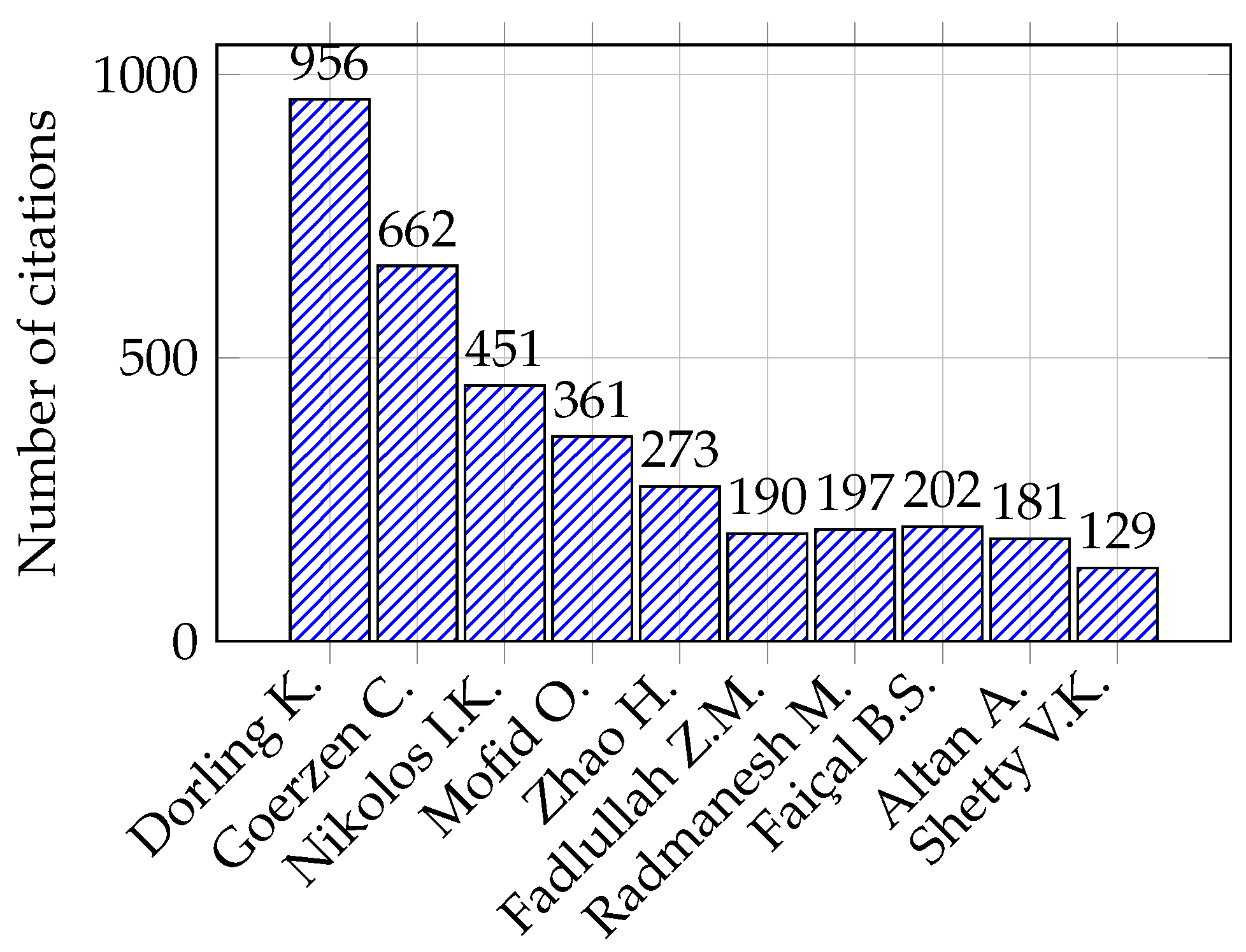
| Main Author | Reference | Citations | Methodology Summary |
|---|---|---|---|
| Dorling | [23] | 956 | Vehicle routing problems for drone delivery. |
| Goerzen | [24] | 662 | Survey of motion planning algorithms for UAV guidance. |
| Nikolos | [25] | 451 | Evolutionary-algorithm-based offline/online path planner for UAV navigation. |
| Mofid | [26] | 361 | Adaptive sliding mode control for quadrotor UAVs. |
| Zhao | [27] | 273 | Deployment algorithms for airborne UAV networks. |
| Fadlullah | [28] | 190 | Dynamic trajectory control algorithm for UAV surveillance. |
| Radmanesh | [29] | 197 | Overview of path-planning and obstacle avoidance strategies in UAVs. |
| Faiçal | [30] | 202 | Adaptive approach for UAV-based pesticide spraying. |
| Altan | [31] | 181 | Performance of metaheuristic optimization algorithms for UAV path planning. |
| Shetty | [32] | 129 | Priority-based assignment and routing of UAVs. |
| Category | Variable/ Parameter | Description |
|---|---|---|
| Position References | , , | Desired position in inertial frame |
| Desired yaw angle | ||
| Position Feedback | x, y, z | Measured position in inertial frame |
| , , | Linear velocity feedback in inertial frame | |
| Attitude References | , | Desired roll and pitch angles |
| Desired yaw angle | ||
| Total thrust command | ||
| Attitude Feedback | , , | Measured Euler angles from IMU |
| p, q, r | Angular velocity feedback in body frame | |
| Control Inputs | , | Roll and pitch setpoints from outer loop |
| , | Commanded yaw rate and thrust | |
| Motor and Physical Parameters | , | Thrust from rotor i and thrust coefficient |
| l, d | Arm length and rotor drag coefficient | |
| Controller Parameters | , | PD gains: proportional and derivative time |
| Transfer function of PD controller | ||
| Optimization Problem | State vector: positions, velocities, angles, rates | |
| Control vector: thrust and torques | ||
| Nonlinear system dynamics function | ||
| Constraints | Bounds on control inputs | |
| Operating limits on state variables |
| Parameter | Value/Description |
|---|---|
| Input signals | Reference trajectory error and system output |
| Number of inputs | 2 (reference, feedback) |
| Input delay taps | 1:3 |
| Output delay taps | 1:3 |
| Hidden layer size | 15 neurons |
| Hidden layer activation | Tangent sigmoid (tansig) |
| Output layer activation | Linear (purelin) |
| Training algorithm | Levenberg–Marquardt (trainlm) |
| Loss function | Mean Squared Error (MSE) |
| Data set size | 1500 samples (3 trajectories, 500 points each) |
| Training/Validation/Test split | 70%/15%/15% |
| Stopping criteria | Validation performance or 1000 epochs |
| Regularization | Early stopping based on validation error |
| Dataset | Observations | MSE | |
|---|---|---|---|
| Training | 700 | 0.0007 | 0.8339 |
| Validation | 150 | 0.0000 | 0.9958 |
| Test | 150 | 0.0017 | 0.7933 |
| Axis | Training Algorithm | Neurons | MSE | Note | |
|---|---|---|---|---|---|
| Z | Lavenberg–Marquardt | 2 | 0.8656 | ||
| 4 | 0.7929 | ||||
| 6 | 0.8670 | ||||
| Bayesian Regularization | 2 | 0.9852 | Best | ||
| 4 | 0.9607 | ||||
| 6 | 0.9400 | ||||
| Scaled Conjugate Gradient | 2 | 0.7449 | |||
| 4 | 0.7721 | ||||
| 6 | 0.6600 | ||||
| X | Lavenberg–Marquardt | 2 | 0.9460 | ||
| 4 | 0.8051 | ||||
| 6 | 0.8168 | ||||
| Bayesian Regularization | 2 | 0.9915 | Best | ||
| 4 | 0.9429 | ||||
| 6 | 0.9751 | ||||
| Scaled Conjugate Gradient | 2 | 0.8748 | |||
| 4 | 0.9150 | ||||
| 6 | 0.8820 | ||||
| Y | Lavenberg–Marquardt | 2 | 0.8393 | ||
| 4 | 0.7876 | ||||
| 6 | 0.9135 | ||||
| Bayesian Regularization | 2 | 0.9843 | Best | ||
| 4 | 0.9593 | ||||
| 6 | 0.9773 | ||||
| Scaled Conjugate Gradient | 2 | 0.8123 | |||
| 4 | 0.6932 | ||||
| 6 | 0.9476 |
| Axis | Input Type | PD Controller | Neural Network |
|---|---|---|---|
| X | Step | 114.47 | 128.08 |
| Sinusoidal | 2.05 | 5.27 | |
| Triangular | 22.63 | 24.07 | |
| Y | Step | 113.82 | 109.15 |
| Sinusoidal | 2.01 | 4.99 | |
| Triangular | 22.33 | 23.77 | |
| Z | Step | 70.96 | 108.52 |
| Sinusoidal | 11.59 | 4.97 | |
| Triangular | 22.35 | 31.41 |
Disclaimer/Publisher’s Note: The statements, opinions and data contained in all publications are solely those of the individual author(s) and contributor(s) and not of MDPI and/or the editor(s). MDPI and/or the editor(s) disclaim responsibility for any injury to people or property resulting from any ideas, methods, instructions or products referred to in the content. |
© 2025 by the authors. Licensee MDPI, Basel, Switzerland. This article is an open access article distributed under the terms and conditions of the Creative Commons Attribution (CC BY) license (https://creativecommons.org/licenses/by/4.0/).
Share and Cite
Pavon, W.; Chavez, J.; Guffanti, D.; Asiedu-Asante, A.B. Unmanned Aerial Vehicle Position Tracking Using Nonlinear Autoregressive Exogenous Networks Learned from Proportional-Derivative Model-Based Guidance. Math. Comput. Appl. 2025, 30, 78. https://doi.org/10.3390/mca30040078
Pavon W, Chavez J, Guffanti D, Asiedu-Asante AB. Unmanned Aerial Vehicle Position Tracking Using Nonlinear Autoregressive Exogenous Networks Learned from Proportional-Derivative Model-Based Guidance. Mathematical and Computational Applications. 2025; 30(4):78. https://doi.org/10.3390/mca30040078
Chicago/Turabian StylePavon, Wilson, Jorge Chavez, Diego Guffanti, and Ama Baduba Asiedu-Asante. 2025. "Unmanned Aerial Vehicle Position Tracking Using Nonlinear Autoregressive Exogenous Networks Learned from Proportional-Derivative Model-Based Guidance" Mathematical and Computational Applications 30, no. 4: 78. https://doi.org/10.3390/mca30040078
APA StylePavon, W., Chavez, J., Guffanti, D., & Asiedu-Asante, A. B. (2025). Unmanned Aerial Vehicle Position Tracking Using Nonlinear Autoregressive Exogenous Networks Learned from Proportional-Derivative Model-Based Guidance. Mathematical and Computational Applications, 30(4), 78. https://doi.org/10.3390/mca30040078