A Family of Newton and Quasi-Newton Methods for Power Flow Analysis in Bipolar Direct Current Networks with Constant Power Loads

Abstract

This paper presents a comprehensive study on the formulation and solution of the power flow problem in bipolar direct current (DC) distribution networks with unbalanced constant power loads. Using the nodal voltage method, a unified nonlinear model is proposed which accurately captures both monopolar and bipolar load configurations as well as the voltage coupling between conductors. The model assumes a solid grounding of the neutral conductor and known system parameters, ensuring reproducibility and physical consistency. Seven iterative algorithms are developed and compared, including three Newton–Raphson-based formulations and four quasi-Newton methods with constant Jacobian approximations. The proposed techniques are validated on two benchmark networks comprising 21 and 85 buses. Numerical results demonstrate that Newton-based methods exhibit quadratic convergence and high accuracy, while quasi-Newton approaches significantly reduce computational time, making them more suitable for large-scale systems. The findings highlight the trade-offs between convergence speed and computational efficiency, and they provide valuable insights for the planning and operation of modern bipolar DC grids.

1. Introduction

1.1. General Context

In recent years, direct current (DC) distribution networks have attracted significant attention due to their improved efficiency and better controllability, as well as technological advancements in power electronics [1,2]. Many distributed energy resources, such as photovoltaic (PV) panels, batteries, and electronic loads, inherently operate in DC, which reduces the need for extensive power conversion stages and improves the overall system performance [3]. These advantages position DC networks as a compelling alternative to conventional alternating current (AC) systems, especially at both high and low voltage levels [4,5]. While high-voltage DC systems are primarily used for long-distance transmission [6], low-voltage DC (LVDC) networks are being increasingly considered for urban and rural distribution systems [7]. Unlike AC systems, DC grids do not require synchronization and are immune to reactive power issues, which results in reduced power losses and enhanced voltage regulation across the network [8].

Within the domain of LVDC networks, bipolar configurations—comprising positive, negative, and neutral conductors—have emerged as a more efficient and flexible alternative to monopolar systems [9]. These networks offer greater reliability and improved fault tolerance while also enabling power sharing between conductors. Despite their advantages, the modeling and analysis of bipolar DC networks remain underdeveloped from the perspective of utilities. In particular, while considerable research has focused on dynamic aspects and converter-level control, the static analysis—specifically the power flow formulation—has received limited attention [10]. Accurate and efficient power flow models are crucial, as they serve as the foundation for planning, operation, and control tasks in electrical systems [11]. The development of robust power flow methods tailored to bipolar LVDC networks is essential to support their integration and widespread adoption in modern distribution systems [12].

1.2. Motivation

The reliable operation and planning of bipolar direct current (DC) distribution networks critically depend on the accurate solution of the power flow problem [13,14]. In these systems, the presence of constant power loads introduces strong nonlinearities due to the inverse voltage–current relationship, which leads to hyperbolic equations far more complex than those found in linear resistive models [15]. Moreover, the bipolar configuration—featuring positive, negative, and neutral conductors—adds another layer of complexity by coupling the voltages across poles and requiring a detailed representation of unbalanced load conditions [16]. These challenges make analytical solutions intractable, especially in large-scale networks with multiple load types and topological variations. Therefore, developing robust and efficient numerical methods is essential to ensure convergence, computational efficiency, and physical realism. Such methods are fundamental for enabling static analysis, voltage regulation, and loss minimization in modern DC grids [17], ultimately supporting the deployment of resilient and intelligent power distribution systems.

On the other hand, the asymmetry of the loads connected between the positive–neutral and negative–neutral poles gives rise to unbalanced conditions in bipolar DC networks, which complicates the power flow calculation [18]. The resulting neutral current induces voltage deviations between the positive and negative poles, meaning that traditional balanced assumptions commonly used in monopolar DC systems are no longer valid. Consequently, load flow analysis must explicitly account for the unbalanced nature of the network to accurately represent operating conditions and ensure reliable solutions.

1.3. Brief Literature Review

In the specialized literature, multiple authors have presented solution methodologies based on numerical methods to deal with the power flow and optimal power flow problems in bipolar DC networks with constant power loads. Some of the most representative algorithms are presented below.

The authors of [19] proposed an optimal power flow (OPF) formulation for bipolar DC microgrids based on a current injection model in order to fully capture the bipolar structure. This formulation employs the output current of distributed generators and pole voltages as decision variables, enabling the linearization of the power flow equations. The OPF minimizes generation costs, voltage imbalance, and network losses. Depending on system characteristics, the problem is modeled as a convex or nonconvex quadratic program. Numerical results demonstrated the method’s effectiveness and low computational burden across various grid scenarios.

The work by [20] addressed the challenges of congestion and asymmetric loading in bipolar DC distribution grids by proposing an exact OPF formulation expressed in terms of voltage and current. This model accounts for the possibility of current flowing through the neutral conductor and supports arbitrary source/load connections between any pair of nodes. Unlike traditional DC models relying on a common ground assumption, the proposed formulation incorporates bilinear cost functions. Consequently, the computation of locational marginal prices (LMPs) is performed as a post-processing step. This approach enables a more accurate pricing mechanism under partial congestion scenarios in bipolar configurations.

In [13], a current injection-based power flow analysis and optimal generation dispatch approach for bipolar DC microgrids was proposed. This study highlighted that, despite voltage balancing at the converter level, significant imbalance can occur at distant buses. To address this issue, the authors developed a Newton–Raphson power flow method based on the static models of the grid components, including voltage balancers, sources, and loads. Furthermore, an optimization problem was formulated using voltage sensitivity derived from the Jacobian matrix to jointly minimize operation costs and voltage imbalance. Simulation results validated the accuracy of the method against PSCAD/EMTDC, demonstrating its effectiveness in steady-state analysis and optimal dispatch.

The study by [10] addressed the challenges of power losses and voltage imbalance in two-phase bipolar DC distribution networks, which rely on a neutral wire for improved efficiency. A power flow formulation based on single-line modeling and nodal analysis was proposed, enabling the system’s steady-state representation. To optimize the placement of unipolar loads across the two poles, a binary integer load redistribution model was developed. This was integrated into a binary integer quadratic multi-objective optimization framework that minimizes both power losses and voltage imbalance. Using the weighted sum method, the problem was solved and validated through case studies involving 15- and 33-bus systems. The results demonstrated the proposal’s superior performance in voltage balancing when compared to conventional iterative approaches.

The work by [21] proposed a Newton–Raphson-based power flow algorithm for bipolar DC microgrids which incorporates current injection modeling and considers grounding schemes and voltage control strategies. Six bus types were defined based on these characteristics, and unknown pole voltages were updated using a unified NR approach. The method achieved high accuracy compared to PSCAD/EMTDC simulations, with low computational effort.

The authors of [22] developed a power flow algorithm for bipolar DC networks that considers unbalanced loads and the presence of a neutral conductor, be it grounded or floating. The method uses a nodal admittance formulation and approximates the nonlinear load–voltage relations via a Taylor series expansion, resulting in a recursive solver with quadratic convergence. Numerical validations on 4-, 21-, and 85-bus systems demonstrated the method’s accuracy and general applicability to radial and meshed topologies, outperforming the traditional successive approximations method.

In [11], the power flow problem for bipolar DC distribution networks with unbalanced constant power loads was addressed while considering two grounding scenarios for the neutral wire: solid grounding at each load point and grounding only at the substation. The problem was solved using the successive approximations method, which was shown to be equivalent to the backward/forward sweep in matrix form. Simulations on 4- and 25-node systems demonstrated the method’s efficiency and suitability for both radial and meshed networks without the need for matrix inversion at each iteration.

The authors of [12] analyzed the power flow problem in radial bipolar DC networks with multiple monopolar and bipolar constant power loads while considering a non-grounded reference pole along the feeder. A triangular recursive formulation was proposed to iteratively compute node voltages, capturing the effects of neutral currents and voltage imbalances. The method exhibited linear convergence under varying load conditions, and numerical tests on 21- and 85-bus systems demonstrated significant differences in voltage profiles and power losses depending on the neutral grounding configuration.

The work by [23] addressed the limitations of conventional Newton methods for power flow analysis when the current protection of converters introduces a non-differentiable behavior. To overcome this issue, the authors proposed a derivative-free fixed-point iterative method capable of handling the saturation effects imposed by converter current limits. The convergence and uniqueness of the solution were rigorously proven using Banach’s fixed-point theorem. Numerical experiments in MATLAB supported the theoretical results and confirmed the method’s effectiveness.

The authors of [24] proposed a graphical interface to solve the power flow problem in unbalanced bipolar DC networks using the successive approximations method. This interface was developed to assist users without programming skills in performing power flow analysis. The study included the formulation of the mathematical model, the implementation of the interface, and its validation using benchmark networks. Numerical results confirmed the accuracy of the proposed tool, matching previously reported solutions with 100% reliability.

The contributions reviewed above constitute a diverse set of methodologies for solving the power flow and OPF problems in bipolar DC networks with constant power loads, wherein Newton–Raphson-based methods have been shown to be accurate and computationally efficient, especially when formulated using current injection models and adapted to different grounding schemes, and recursive formulations based on Taylor or hyperbolic approximations enable quadratic convergence and general applicability to both radial and meshed topologies. Additionally, several works addressed optimization aspects, such as the minimization of generation costs, voltage imbalance, and power losses, using convex or nonconvex quadratic programming. Triangular iterative solvers and fixed-point methods have been proposed to handle the non-differentiable behaviors introduced by converter protection mechanisms. Moreover, graphical tools have been developed to enhance accessibility for non-programmers, confirming the practical applicability of the proposed methods. Overall, the literature demonstrates the robustness and versatility of numerical techniques for analyzing and optimizing bipolar DC grids.

Despite these valuable contributions, there are still several limitations that remain unaddressed. Most of the existing methods rely on specific Jacobian approximations or case-dependent linearizations without analyzing structural implications on convergence and conditioning. In addition, few works explore generalized frameworks that simultaneously account for monopolar and bipolar load configurations, and even fewer provide a systematic comparison of exact vs. approximated Jacobian formulations. Moreover, the computational trade-offs between accuracy, convergence speed, and matrix conditioning are rarely discussed in depth. This article addresses these gaps by proposing a family of Newton and quasi-Newton methods specifically designed for bipolar DC networks, supported by a convergence analysis and numerical validations that highlight the structural impact of the Jacobian on performance.

1.4. Contributions

This article proposes a general model for the power flow analysis in bipolar DC grids. Its contributions are twofold:

• A unified power flow formulation for bipolar DC networks that considers monopolar and bipolar constant power loads. This model captures the nonlinear relationship between voltage and current via a generalized expression that integrates the effects of solidly grounded neutral wires. This formulation is suitable for both radial and meshed topologies and serves as the basis for Newton and quasi-Newton iterative solvers.
• A comparative study of multiple Newton and quasi-Newton power flow methods applied to two benchmark networks comprising 21 and 85 buses. The proposed methods demonstrate fast convergence and computational efficiency, with the Newton-based algorithms exhibiting quadratic convergence and the quasi-Newton methods offering lower computational costs through constant Jacobian approximations.

Within the scope of this research, it is assumed that the neutral wire is solidly grounded at every node of the bipolar DC distribution network. Furthermore, the systems under study do not include additional voltage-controlled nodes beyond the slack bus. The analysis also considers that all the parametric information of the test systems—such as constant power loads and line resistances—is fully known and accurately specified, ensuring a well-defined and reproducible evaluation of the proposed power flow methodologies.

Note that the free software studied in this research allows electrical engineering students and researchers to validate the proposed analysis on bipolar power flow methods by using the software and contact information provided in

Table 1. Code metadata.

Current code version	V1.0
Permanent link to code/repository used for this code version	https://github.com/odmontoya/Newton-Raphson-Family-Bipolar-DC-Networks, accessed on 4 May 2025
Legal code license	MIT License
Code versioning system used	Git
Programming languages, tools, and libraries used	MATLAB R2024b
Compilation requirements and runtime environment	MATLAB (any OS with MATLAB R2024b or later)
Contact email for support	odmontoyag@udistrital.edu.co, accessed on 4 May 2025

.

A key contribution of this work is the development of a unified formulation that integrates multiple modeling approaches within a single mathematical framework. This formulation enables the simultaneous treatment of various system components and constraints that were previously addressed in a fragmented manner in the literature. By consolidating these aspects, the proposed framework enhances the consistency, generality, and computational efficiency of the analysis and optimization process. This unified approach not only simplifies implementation but also provides a foundation for extending the methodology to accommodate emerging technologies and operational scenarios, thereby broadening the applicability and impact of the proposed solution.

1.5. Article Structure

The remainder of this document is organized as follows: Section 2 introduces the general formulation of the power flow problem for bipolar DC grids, incorporating constant power terminals and unbalanced load conditions through the classical nodal voltage method. This formulation leads to a generalized nonlinear power flow equation. Section 3 provides the theoretical background of the Newton–Raphson method and details the seven proposed solution strategies—three based on Newton–Raphson algorithms and four based on quasi-Newton approximations. Section 4 describes the main features of the test systems used (i.e., 21- and 85-bus bipolar DC distribution networks). Section 5 presents the numerical results obtained, including average processing times, calculated power losses, and voltage profile behaviors, as well as a convergence analysis through graphical representation. Finally, Section 6 summarizes the main conclusions of this study and outlines potential directions for future research.

2. Power Flow Formulation for Bipolar DC Networks

In this section, all matrices are denoted using bold uppercase symbols, while subscripts and superscripts are used to indicate nodes and iteration indices, respectively.

The formulation of the power flow problem for bipolar DC distribution networks is based on the nodal admittance representation, specifically employing the branch-to-node admittance matrix approach as introduced in [8]. The fundamental relationship between nodal voltages and injected currents is captured by the admittance matrix, as detailed in Equation (1). For more details, see [25] [Cap. 4].

$$\left[\begin{array}{c}{\mathbf{I}}_s\\ -{\mathbf{I}}_d\end{array}\right]=\left[\begin{array}{cc}{\mathbf{G}}_{ss}& {\mathbf{G}}_{sd}\\ {\mathbf{G}}_{ds}& {\mathbf{G}}_{dd}\end{array}\right]\left[\begin{array}{c}{\mathbf{V}}_s\\ {\mathbf{V}}_d\end{array}\right],$$

(1)

In this formulation, the vector ${\mathbf{I}}_s$ represents the current injections at the positive and negative poles of the voltage-controlled nodes, while ${\mathbf{I}}_d$ denotes the currents drawn by the loads connected to both poles of the bipolar DC network. The admittance matrix ${\mathbf{G}}_{pn}$ is partitioned into four submatrices: ${\mathbf{G}}_{ss}$, ${\mathbf{G}}_{sd}$, ${\mathbf{G}}_{ds}$, and ${\mathbf{G}}_{dd}$, each describing the electrical relationships between source and demand nodes within the system. The vector ${\mathbf{V}}_s$ contains the voltages imposed by the controlled sources, while ${\mathbf{V}}_d$ comprises the voltage variables associated with the demand-side nodes.

It is important to note that the sign conventions applied to the second row of the current expressions for the demand nodes reflects the direction of current flow: a positive net current indicates inflow at a node, whereas a negative value corresponds to an outflow due to the presence of loads.

2.1. General Power Flow Formula

A general expression for the power flow solution can be derived by manipulating the second row of Equation (1) to isolate the vector ${\mathbf{V}}_{d,pn}$, which represents the voltages at the demand nodes [11]. This procedure enables the explicit calculation of these voltages, as described in [26]:

$$\begin{array}{c}\hfill {\mathbf{G}}_{dd}{\mathbf{V}}_d+{\mathbf{G}}_{ds}{\mathbf{V}}_s+{\mathbf{I}}_d=0\end{array}$$

(2)

2.2. Demanded Current Calculation

One of the main challenges in solving the power flow equations of bipolar DC networks arises from the nonlinear, hyperbolic relationship between nodal voltages and constant power demands [11]. This section outlines the way in which the current associated with the constant power loads is computed, both when they are connected between a single pole (positive or negative) and the ground, and when the connection spans between both poles.

For a given node k where loads are individually connected between each pole and the ground, the corresponding current injections are calculated using Equations (3) and (4) [22]:

$$\begin{array}{c}\hfill I_{dk,p}={\displaystyle \frac{P_{dk,p}}{V_{dk,p}}},\end{array}$$

(3)

$$\begin{array}{c}\hfill I_{dk,n}={\displaystyle \frac{P_{dk,n}}{V_{dk,n}}},\end{array}$$

(4)

where $I_{dk,p}$ and $I_{dk,n}$ represent the currents injected at time t into the positive and negative poles, respectively; the terms $P_{dk,p}$ and $P_{dk,n}$ denote the constant power demand associated with each pole; and $V_{dk,p}$ and $V_{dk,n}$ are the corresponding voltage magnitudes.

If each node in the system is exclusively equipped with loads connected between either pole and the neutral point, the current demand expressions in Equations (3) and (4) can be generalized into a compact matrix form [11]:

$$\begin{array}{c}\hfill {\mathbf{I}}_{dk,pn}={\mathrm{diag}}^{-1}\left({\mathbf{V}}_{dk,pn}\right){\mathbf{P}}_{dk,pn},\end{array}$$

(5)

where ${\mathbf{P}}_{dk,pn}$ is a vector containing the constant power consumption associated with each pole at node k; the vector ${\mathbf{I}}_{dk,pn}$ represents the corresponding current demands during iteration t; and ${\mathbf{V}}_{dk,pn}$ includes the positive and negative voltage values at node k for the same iteration.

In scenarios where a load is connected between the positive and negative poles at a given node k, the associated current injections can be expressed as follows:

$$\begin{array}{c}\hfill I_{dk,p}={\displaystyle \frac{P_{dk,pn}}{V_{dk,p}-V_{dk,n}}},\end{array}$$

(6)

$$\begin{array}{c}\hfill I_{dk,n}={\displaystyle \frac{P_{dk,pn}}{V_{dk,n}-V_{dk,p}}},\end{array}$$

(7)

where $P_{dk,pn}$ denotes the constant power load connected between the two poles.

When all constant power loads in the system are exclusively configured between poles, the above expressions can be generalized into the compact matrix form shown below [12]:

$$\begin{array}{c}\hfill {\mathbf{I}}_{dk,pn}={\mathrm{diag}}^{-1}\left(\mathbf{H}{\mathbf{V}}_{d,pn}\right){\mathbf{P}}_{dk,pn},\end{array}$$

(8)

with matrix $\mathbf{H}$ defined as follows:

$$\begin{array}{c}\hfill \mathbf{H}=\left[\begin{array}{cc}1& -1\\ -1& 1\end{array}\right].\end{array}$$

(9)

This formulation captures the voltage difference between poles and applies it consistently to compute the corresponding line-to-line current demands.

Remark 1. 

When a node includes both line-to-ground and line-to-line constant power loads, its total current demand corresponds to the algebraic sum of the individual contributions [22]. Specifically, the total current in each pole is obtained by summing the line-to-ground current components given in Equations (6) and (7) with the line-to-line components expressed in Equation (8).

Note that, in order to obtain the general power flow formula (see Equation (2)) solely as a function of the demanded voltage vector ${\mathbf{V}}_d$, the demanded currents ${\mathbf{I}}_d$ for monopolar and bipolar DC loads presented in Equations (6) and (10) can be generalized as follows:

$$\begin{array}{c}\hfill {\mathbf{I}}_d={\mathrm{diag}}^{-1}\left({\mathbf{V}}_d\right){\mathbf{P}}_{dm}+{\mathrm{diag}}^{-1}\left(\mathbf{M}{\mathbf{V}}_d\right){\mathbf{P}}_{db},\end{array}$$

(10)

where $\mathbf{M}$ is a matrix composed of the submatrices H in its diagonal, i.e.,

$$\begin{array}{c}\hfill \mathbf{M}=\left[\begin{array}{cccc}\mathbf{H}& {\mathbf{0}}_{2\times 2}& \cdots & {\mathbf{0}}_{2\times 2}\\ {\mathbf{0}}_{2\times 2}& \mathbf{H}& \cdots & {\mathbf{0}}_{2\times 2}\\ ⋮& \ddots & \ddots & ⋮\\ {\mathbf{0}}_{2\times 2}& {\mathbf{0}}_{2\times 2}& \cdots & \mathbf{H}\end{array}\right];\end{array}$$

(11)

where ${\mathbf{P}}_{dm}$ and ${\mathbf{P}}_{db}$ are vectors containing monopolar and bipolar constant power loads ordered by node; and ${\mathbf{0}}_{2\times 2}$ denotes a $2\times 2$ zero matrix.

Considering the definitions in (10) and (11), the general power flow formula in (2) takes the following form:

$$\begin{array}{c}\hfill \mathbf{F}\left({\mathbf{V}}_d\right)={\mathbf{G}}_{dd}{\mathbf{V}}_d+{\mathbf{G}}_{ds}{\mathbf{V}}_s+{\mathrm{diag}}^{-1}\left({\mathbf{V}}_d\right){\mathbf{P}}_{dm}+{\mathrm{diag}}^{-1}\left(\mathbf{M}{\mathbf{V}}_d\right){\mathbf{P}}_{db}=0.\end{array}$$

(12)

Remark 2. 

It is worth noting that the second row of Equation (12) captures the relationship between the current demands and the corresponding voltage variables at the load nodes. Due to the nonlinear nature of this expression, its solution typically requires the use of an iterative numerical method.

3. Theoretical Background and Power Flow Formulations

This section presents the theoretical foundations and convergence analysis of the Newton–Raphson and quasi-Newton methods applied to the solution of nonlinear power flow problems for bipolar DC distribution networks. These networks may include multiple monopolar and bipolar constant power terminals. The methods considered rely on successive approximations derived from Taylor series expansions to iteratively solve the vector-valued nonlinear system of equations.

3.1. Multivariate Formulation and Taylor Expansion

Consider a nonlinear system of equations given by $\mathbf{F}\left(\mathbf{x}\right)=\mathbf{0}$, where $\mathbf{F}:{\mathbb{R}}^n\to {\mathbb{R}}^n$ is a continuously differentiable vector-valued function and $\mathbf{x}\in {\mathbb{R}}^n$ is the vector of unknowns [27]. To derive the Newton–Raphson method, one starts with the multivariable Taylor series expansion of $\mathbf{F}\left(\mathbf{x}\right)$ around a point ${\mathbf{x}}_k$ [28]:

$$\begin{array}{c}\hfill \mathbf{F}\left(\mathbf{x}\right)\approx \mathbf{F}\left({\mathbf{x}}_k\right)+\mathbf{J}\left({\mathbf{x}}_k\right)(\mathbf{x}-{\mathbf{x}}_k)+\mathbf{O}(\parallel \mathbf{x}-{\mathbf{x}}_k{\parallel }^2),\end{array}$$

(13)

where $\mathbf{J}\left({\mathbf{x}}_k\right)$ denotes the Jacobian matrix of partial derivatives evaluated at ${\mathbf{x}}_k$. Neglecting higher-order terms and setting $\mathbf{F}\left({\mathbf{x}}_{k+1}\right)=\mathbf{0}$ yields the following Newton–Raphson iteration formula:

$$\begin{array}{c}\hfill {\mathbf{x}}_{k+1}={\mathbf{x}}_k-{\mathbf{J}}^{-1}\left({\mathbf{x}}_k\right)\mathbf{F}\left({\mathbf{x}}_k\right).\end{array}$$

(14)

This iterative method is known for its quadratic convergence when the Jacobian is nonsingular and the initial guess is sufficiently close to the solution [29]. In practical applications, particularly in large-scale systems such as DC networks, the burden associated with computing and inverting the Jacobian motivates the use of quasi-Newton methods [12]. These approaches iteratively update an approximation of the Jacobian (or its inverse), thus reducing computational complexity while retaining favorable convergence properties.

3.2. Newton–Raphson Bipolar Power Flow Formulations

This subsection presents three alternative formulations to solve the bipolar DC power flow problem. Each formulation rewrites the general nodal equations to model constant power terminals under different configurations, enabling the use of Newton–Raphson-based iterative methods.

3.2.1. First Newton–Raphson Formulation

To obtain the generic Newton–Raphson iterative approach, Equation (12) is rewritten as follows:

$$\begin{array}{c}\hfill {\mathbf{F}}_1\left({\mathbf{V}}_d\right)={\mathbf{G}}_{dd}{\mathbf{V}}_d+{\mathbf{G}}_{ds}{\mathbf{V}}_s+{\mathrm{diag}}^{-1}\left({\mathbf{V}}_d\right){\mathbf{P}}_{dm}+{\mathrm{diag}}^{-1}\left(\mathbf{M}{\mathbf{V}}_d\right){\mathbf{P}}_{db}=\mathbf{0}.\end{array}$$

(15)

The Jacobian matrix is given by

$$\begin{array}{c}\hfill {\mathbf{J}}_{{\mathbf{F}}_1}\left({\mathbf{V}}_d\right)={\mathbf{G}}_{dd}-{\mathrm{diag}}^{-2}\left({\mathbf{V}}_d\right)\mathrm{diag}\left({\mathbf{P}}_{dm}\right)-{\mathrm{diag}}^{-2}\left(\mathbf{M}{\mathbf{V}}_d\right)\mathrm{diag}\left({\mathbf{P}}_{db}\right)\mathbf{M},\end{array}$$

(16)

which implies that the iterative formula for the first Newton–Raphson method (NRM1) takes the following structure:

The Newton–Raphson update is

$$\begin{array}{c}\hfill {\mathbf{V}}_d^{k+1}={\mathbf{V}}_d^k-{\left[{\mathbf{J}}_{{\mathbf{F}}_1}\left({\mathbf{V}}_d^k\right)\right]}^{-1}{\mathbf{F}}_1\left({\mathbf{V}}_d^k\right),\end{array}$$

(17)

which is repeated until $\parallel {\mathbf{V}}_d^{k+1}-{\mathbf{V}}_d^k{\parallel }_{\infty }\le ϵ$.

3.2.2. Second Newton–Raphson Formulation

This formulation simplifies Equation (12), pre-multiplying it by $\mathrm{diag}\left({\mathbf{V}}_d\right)$ in order to reduce the computational complexity of the Jacobian evaluation and solution process, thereby enabling faster iterations. However, it may also impact convergence speed and robustness. Its inclusion allows for a comparative analysis between structural simplification and numerical performance in practical scenarios. This formulation includes the following set of nonlinear equations:

$$\begin{array}{c}\hfill {\mathbf{F}}_2\left({\mathbf{V}}_d\right)=\mathrm{diag}\left({\mathbf{V}}_d\right)\left({\mathbf{G}}_{dd}{\mathbf{V}}_d+{\mathbf{G}}_{ds}{\mathbf{V}}_s+{\mathrm{diag}}^{-1}\left(\mathbf{M}{\mathbf{V}}_d\right){\mathbf{P}}_{db}\right)+{\mathbf{P}}_{dm}=\mathbf{0}.\end{array}$$

(18)

$$\begin{array}{c}\hfill \mathbf{g}\left({\mathbf{V}}_d\right)={\mathbf{G}}_{dd}{\mathbf{V}}_d+{\mathbf{G}}_{ds}{\mathbf{V}}_s+{\mathrm{diag}}^{-1}\left(\mathbf{M}{\mathbf{V}}_d\right){\mathbf{P}}_{db},\end{array}$$

(19)

yields the Jacobian as follows:

$$\begin{array}{c}\hfill {\mathbf{J}}_{{\mathbf{F}}_2}\left({\mathbf{V}}_d\right)=\mathrm{diag}\left(\mathbf{g}\left({\mathbf{V}}_d\right)\right)+\mathrm{diag}\left({\mathbf{V}}_d\right)\left[{\mathbf{G}}_{dd}-{\mathrm{diag}}^{-2}\left(\mathbf{M}{\mathbf{V}}_d\right)\mathrm{diag}\left({\mathbf{P}}_{db}\right)\mathbf{M}\right].\end{array}$$

(20)

The iterative formula is

$$\begin{array}{c}\hfill {\mathbf{V}}_d^{k+1}={\mathbf{V}}_d^k-{\left[{\mathbf{J}}_{{\mathbf{F}}_2}\left({\mathbf{V}}_d^k\right)\right]}^{-1}{\mathbf{F}}_2\left({\mathbf{V}}_d^k\right).\end{array}$$

(21)

3.2.3. Third Newton–Raphson Formulation

This formulation seeks to introduce a more aggressive decoupling in the Jacobian formulation by pre-multiplying Equation (12) by $\mathrm{diag}\left(\mathbf{M}{\mathbf{V}}_d\right)$. This variant has shown potential for implementation in modularized solvers; while it could sacrifice accuracy in the representation of coupling effects, it significantly simplifies the algebraic structure. Its formulation takes the following form:

$$\begin{array}{c}\hfill {\mathbf{F}}_3\left({\mathbf{V}}_d\right)=\mathrm{diag}\left(\mathbf{M}{\mathbf{V}}_d\right)\left({\mathbf{G}}_{dd}{\mathbf{V}}_d+{\mathbf{G}}_{ds}{\mathbf{V}}_s+{\mathrm{diag}}^{-1}\left({\mathbf{V}}_d\right){\mathbf{P}}_{dm}\right)+{\mathbf{P}}_{db}=\mathbf{0}.\end{array}$$

(22)

With

$$\begin{array}{c}\hfill \mathbf{g}\left({\mathbf{V}}_d\right)={\mathbf{G}}_{dd}{\mathbf{V}}_d+{\mathbf{G}}_{ds}{\mathbf{V}}_s+{\mathrm{diag}}^{-1}\left({\mathbf{V}}_d\right){\mathbf{P}}_{dm},\end{array}$$

(23)

the Jacobian is

$$\begin{array}{c}\hfill {\mathbf{J}}_{{\mathbf{F}}_3}\left({\mathbf{V}}_d\right)=\mathrm{diag}\left(\mathbf{g}\left({\mathbf{V}}_d\right)\right)\mathbf{M}+\mathrm{diag}\left(\mathbf{M}{\mathbf{V}}_d\right)\left[{\mathbf{G}}_{dd}-{\mathrm{diag}}^{-2}\left({\mathbf{V}}_d\right)\mathrm{diag}\left({\mathbf{P}}_{dm}\right)\right].\end{array}$$

(24)

The update step takes the following form:

$$\begin{array}{c}\hfill {\mathbf{V}}_d^{k+1}={\mathbf{V}}_d^k-{\left[{\mathbf{J}}_{{\mathbf{F}}_3}\left({\mathbf{V}}_d^k\right)\right]}^{-1}{\mathbf{F}}_3\left({\mathbf{V}}_d^k\right).\end{array}$$

(25)

Each formulation provides a structurally distinct approach for modeling bipolar DC systems while retaining compatibility with the Newton–Raphson method. The selection of one such formulation may impact convergence behavior and numerical stability depending on system topology and loading conditions.

Remark 3. 

The Newton–Raphson-based power flow formulations presented above are not unique. Several alternative expressions can be derived from the General Nodal Power Flow Equation (12), depending on how the nonlinear terms are manipulated. This flexibility allows developing additional iterative algorithms tailored to specific network configurations or numerical properties.

3.3. Quasi-Newton Methods with Constant Jacobians

To reduce the computational cost associated with evaluating and inverting the Jacobian matrix at each iteration of the Newton–Raphson method, a quasi-Newton strategy can be adopted. This strategy assumes a constant Jacobian matrix ${\mathbf{A}}_{01}$, evaluated at the initial guess ${\mathbf{V}}_d^0$ and used throughout all iterations. This approximation avoids the repeated computation of derivatives and matrix inversions, thus simplifying the numerical implementation while maintaining acceptable accuracy in most practical cases.

For a given formulation ${\mathbf{F}}_i\left({\mathbf{V}}_d\right)$, the quasi-Newton iteration is

$$\begin{array}{c}\hfill {\mathbf{V}}_d^{k+1}={\mathbf{V}}_d^k-{\mathbf{A}}_{0i}^{-1}{\mathbf{F}}_i\left({\mathbf{V}}_d^k\right),\end{array}$$

(26)

where ${\mathbf{A}}_{0i}={\mathbf{J}}_{{\mathbf{F}}_i}\left({\mathbf{V}}_d^0\right)$ is the Jacobian evaluated once at the initial voltage vector ${\mathbf{V}}_d^0$ and kept constant for all iterations $k\ge 0$.

This method is particularly beneficial when the initial condition ${\mathbf{V}}_d^0$ is close to the solution or when the nonlinearities of the problem are mild. Despite sacrificing quadratic convergence, this approach often results in significantly faster computation.

3.4. Quasi-Newton Formulations

The following expressions represent the constant Jacobian matrices ${\mathbf{A}}_{0i}$ evaluated at the initial guess ${\mathbf{V}}_d^0$, which correspond to each quasi-Newton method and are explained below.

3.4.1. First Quasi-Newton Method

This quasi-Newton algorithm is obtained when ${\mathbf{J}}_{{\mathbf{F}}_1}\left({\mathbf{V}}_d\right)$ is evaluated at the initial guess ${\mathbf{V}}_d^0$, i.e.,

$${\mathbf{A}}_{01}={\mathbf{J}}_{{\mathbf{F}}_1}\left({\mathbf{V}}_d^0\right)={\mathbf{G}}_{dd}-{\mathrm{diag}}^{-2}\left({\mathbf{V}}_d^0\right)\mathrm{diag}\left({\mathbf{P}}_{dm}\right)-{\mathrm{diag}}^{-2}\left(\mathbf{M}{\mathbf{V}}_d^0\right)\mathrm{diag}\left({\mathbf{P}}_{db}\right)\mathbf{M},$$

(27)

which produces the following iterative formula:

$$\begin{array}{c}\hfill {\mathbf{V}}_d^{k+1}={\mathbf{V}}_d^k-{\mathbf{A}}_{01}^{-1}{\mathbf{F}}_1\left({\mathbf{V}}_d^k\right).\end{array}$$

(28)

3.4.2. Second Quasi-Newton Method

This quasi-Newton method is derived from the second Newton formulation by fixing the simplified Jacobian and using it across all iterations, following a quasi-Newton update scheme. The objective of including this formulation is to analyze the impact of reusing a simplified Jacobian on convergence behavior and the iteration count, particularly in networks with low dynamic variability or when computational resources are limited. The formulation of second quasi-Newton approximation is obtained when ${\mathbf{J}}_{{\mathbf{F}}_2}\left({\mathbf{V}}_d\right)$ is evaluated at the initial guess ${\mathbf{V}}_d^0$, i.e.,

$$\begin{array}{cc}\hfill {\mathbf{A}}_{02}={\mathbf{J}}_{{\mathbf{F}}_2}\left({\mathbf{V}}_d^0\right)=& \mathrm{diag}\left({\mathbf{G}}_{dd}{\mathbf{V}}_d^0+{\mathbf{G}}_{ds}{\mathbf{V}}_s+{\mathrm{diag}}^{-1}\left(\mathbf{M}{\mathbf{V}}_d^0\right){\mathbf{P}}_{db}\right)\hfill \\ & +\mathrm{diag}\left({\mathbf{V}}_d^0\right)\left[{\mathbf{G}}_{dd}-{\mathrm{diag}}^{-2}\left(\mathbf{M}{\mathbf{V}}_d^0\right)\mathrm{diag}\left({\mathbf{P}}_{db}\right)\mathbf{M},\right]\hfill \end{array}$$

(29)

which yields the following iterative formula:

$$\begin{array}{c}\hfill {\mathbf{V}}_d^{k+1}={\mathbf{V}}_d^k-{\mathbf{A}}_{02}^{-1}{\mathbf{F}}_2\left({\mathbf{V}}_d^k\right),\end{array}$$

(30)

3.4.3. Third Quasi-Newton Method

The third quasi-Newton approach extends the decoupling strategy of the third Newton formulation into the quasi-Newton framework. This is the most computationally lightweight variant among the proposed methods. Although it could provide slower convergence due to the strong approximation of the Jacobian structure, its inclusion is relevant for illustrating the lower performance bound when computational simplicity is prioritized over accuracy. The formulation of the second quasi-Newton approximation is reached by evaluating ${\mathbf{V}}_d^0$ in ${\mathbf{J}}_{{\mathbf{F}}_3}\left({\mathbf{V}}_d\right)$ at the initial guess, i.e.,

$$\begin{array}{cc}\hfill {\mathbf{A}}_{03}=& \mathrm{diag}\left({\mathbf{G}}_{dd}{\mathbf{V}}_d^0+{\mathbf{G}}_{ds}{\mathbf{V}}_s+{\mathrm{diag}}^{-1}\left({\mathbf{V}}_d^0\right){\mathbf{P}}_{dm}\right)\mathbf{M}\hfill \\ & +\mathrm{diag}\left(\mathbf{M}{\mathbf{V}}_d^0\right)\left[{\mathbf{G}}_{dd}-{\mathrm{diag}}^{-2}\left({\mathbf{V}}_d^0\right)\mathrm{diag}\left({\mathbf{P}}_{dm}\right)\right],\hfill \end{array}$$

(31)

which generates the following iterative power flow formula:

$$\begin{array}{c}\hfill {\mathbf{V}}_d^{k+1}={\mathbf{V}}_d^k-{\mathbf{A}}_{03}^{-1}{\mathbf{F}}_4\left({\mathbf{V}}_d^k\right).\end{array}$$

(32)

3.4.4. Fourth Quasi-Newton Method

The fourth quasi-Newton formulation approximates ${\mathbf{J}}_{{\mathbf{F}}_3}\left({\mathbf{V}}_d\right)$ by simplifying it as a constant matrix without evaluating the initial guess, i.e.,

$$\begin{array}{c}\hfill {\mathbf{A}}_{04}={\mathbf{G}}_{dd},\end{array}$$

(33)

which yields the following iterative power flow formula:

$$\begin{array}{c}\hfill {\mathbf{V}}_d^{k+1}={\mathbf{V}}_d^k-{\mathbf{A}}_{04}^{-1}{\mathbf{F}}_1\left({\mathbf{V}}_d^k\right).\end{array}$$

(34)

Remark 4. 

This quasi-Newton algorithm, i.e., the Iterative Formula (34), corresponds to the fixed-point formulation (the successive approximations power flow method) reported by the authors of [11], which ensures convergence by applying the Banach fixed-point theorem.

Note that, for all the possible approximations of the Jacobian matrices, the iterative procedure is repeated until the convergence criterion is met, i.e., $\parallel {\mathbf{V}}_d^{k+1}-{\mathbf{V}}_d^k{\parallel }_{\infty }\le ϵ$.

3.5. Solution Procedure

For a better understanding of the proposed power flow solutions, Algorithm 1 summarizes the main steps involved in solving the power flow problem for bipolar DC networks using both Newton and quasi-Newton methods. The general procedure consists of iteratively solving a linearized system of equations, based on either the exact Jacobian or an approximate version, until the convergence criteria are satisfied. The structure of the algorithm is sufficiently general to encompass the different variants of the Newton and quasi-Newton formulations analyzed in this work.

Algorithm 1: Newton and quasi-Newton power flow solver for bipolar DC networks.

1: Input: Network data, load parameters, tolerance $ϵ$, maximum iterations $k_{max}$   2: Initialize voltage estimates ${\mathbf{v}}^{\left(0\right)}$   3: Set iteration counter $k\leftarrow 0$   4: while $\parallel {\mathbf{V}}_d^{k+1}-{\mathbf{V}}_d^k{\parallel }_{\infty }\le ϵ$ or $k\ge k_{max}$ do   5:     Compute the mismatch vector $\mathbf{F}\left({\mathbf{V}}_{\mathbf{d}}^{\left(k\right)}\right)$   6:     Evaluate or approximate the Jacobian matrix $\mathbf{J}\left({\mathbf{V}}_{\mathbf{d}}^{\left(k\right)}\right)$, e.g., using Equation (16) for the first Newton–Raphson formulation, Equation (20) for the second Newton–Raphson formulation, Equation (22) for the third Newton–Raphson formulation, or Equations (27), (29), and (31), or (33) for the quasi-Newton methods.   7:     Update voltages: ${\mathbf{V}}_{\mathbf{d}}^{(k+1)}={\mathbf{V}}_{\mathbf{d}}^{\left(k\right)}-\mathbf{J}{\left({\mathbf{V}}_{\mathbf{d}}^{\left(k\right)}\right)}^{-1}\mathbf{F}\left({\mathbf{V}}_{\mathbf{d}}^{\left(k\right)}\right)$   8:     Update iteration counter: $k\leftarrow k+1$   9: end while 10: Output: Final voltage vector ${\mathbf{v}}^{\left(k\right)}$

Remark 5. 

In Algorithm 1, for the Newton methods, the Jacobian is updated at each iteration, whereas, in the quasi-Newton methods, the Jacobian is kept constant or approximated using specific strategies.

4. Test Feeder Characteristics

To assess the performance and applicability of the proposed power flow methodology for bipolar DC networks, two test systems were considered. The first was a 21-bus medium-voltage distribution network originally developed for balanced conditions and adapted in this study to incorporate unbalanced line-to-ground loads [11], and the second was a bipolar 85-bus network, which included a greater number of nodes and more complex load arrangements [22]. In both cases, the slack buses operated symmetrically with voltages of $\pm 1\mathrm{kV}$ and $\pm 11\mathrm{kV}$, respectively. The electrical configurations and parametric data for each system are provided to support the numerical validation.

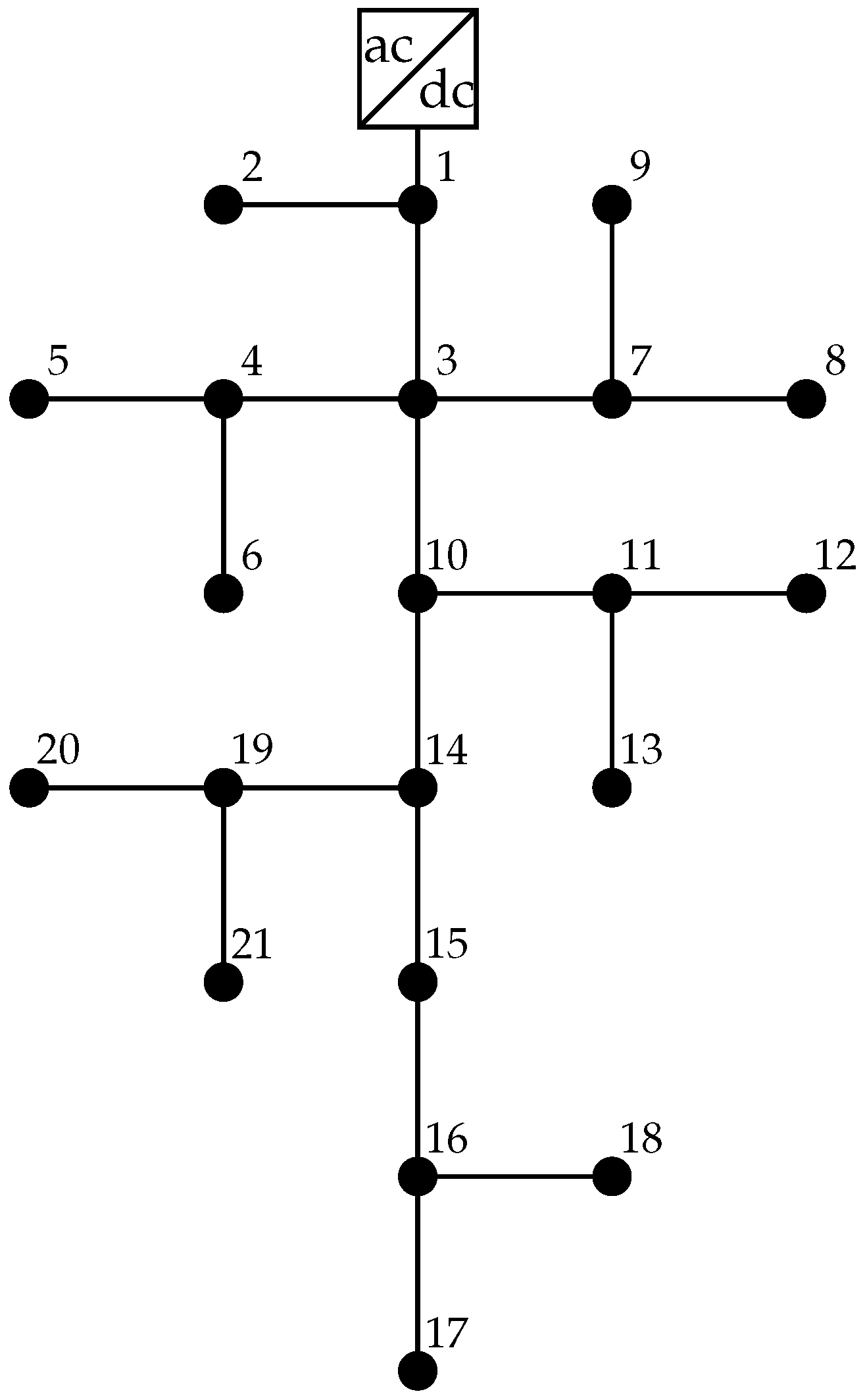
4.1. The 21-Bus Grid

To evaluate the computational performance of the proposed power flow methodology for asymmetric bipolar DC networks, a modified test system was employed. This network consisted of 21 nodes and 20 constant power loads and was initially designed for balanced DC power flow analysis [26]. In this study, the test system was adapted to incorporate unbalanced line-to-ground loads, enabling the assessment of the method under asymmetric operating conditions. The electrical layout of the adapted feeder is depicted in Figure 1.

In this 21-bus test system, the slack bus operates symmetrically with voltage levels of $\pm 1\mathrm{kV}$ on the positive and negative poles. The corresponding electrical parameters of the feeder are detailed in

Table 2. Parametric information regarding lines and loads for the 21-bus system.

Node	Node	${\mathit{R}}_{\mathit{jk}}$	${\mathit{P}}_{\mathit{dk},\mathit{po}}$	${\mathit{P}}_{\mathit{dk},\mathit{no}}$	${\mathit{P}}_{\mathit{dk},\mathit{pn}}$	Node	Node	${\mathit{R}}_{\mathit{jk}}$	${\mathit{P}}_{\mathit{dk},\mathit{po}}$	${\mathit{P}}_{\mathit{dk},\mathit{no}}$	${\mathit{P}}_{\mathit{dk},\mathit{pn}}$
$\mathit{j}$	$\mathit{k}$	($\mathrm{\Omega }$)	(kW)	(kW)	(kW)	$\mathit{j}$	$\mathit{k}$	($\mathrm{\Omega }$)	(kW)	(kW)	(kW)
1	2	0.053	70	100	0	11	12	0.079	68	70	0
1	3	0.054	0	0	0	11	13	0.078	10	0	75
3	4	0.054	36	40	120	10	14	0.083	0	0	0
4	5	0.063	4	0	0	14	15	0.065	22	30	0
4	6	0.051	36	0	0	15	16	0.064	23	10	0
3	7	0.037	0	0	0	16	17	0.074	43	0	60
7	8	0.079	32	50	0	16	18	0.081	34	60	0
7	9	0.072	80	0	100	14	19	0.078	9	15	0
3	10	0.053	0	10	0	19	20	0.084	21	10	50
10	11	0.038	45	30	0	19	21	0.082	21	20	0

.

4.2. The 85-Bus Grid

The 85-bus test system used in this study corresponds to the bipolar DC adaptation presented by the authors of [22]. In this configuration, the substation is positioned at node 1, supplying voltages of $\pm 11\mathrm{kV}$ to the positive and negative poles, respectively, while maintaining the neutral point at $0\mathrm{V}$. The electrical layout of the adapted 85-bus bipolar network is illustrated in Figure 2.

The branch and load parameters associated with this test feeder are provided in

Table 3. Parametric information regarding lines and loads for the 85-bus system.

Node	Node	${\mathit{R}}_{\mathit{jk}}$	${\mathit{P}}_{\mathit{dk},\mathit{po}}$	${\mathit{P}}_{\mathit{dk},\mathit{no}}$	${\mathit{P}}_{\mathit{dk},\mathit{pn}}$	Node	Node	${\mathit{R}}_{\mathit{jk}}$	${\mathit{P}}_{\mathit{dk},\mathit{po}}$	${\mathit{P}}_{\mathit{dk},\mathit{no}}$	${\mathit{P}}_{\mathit{dk},\mathit{pn}}$	Node	Node	${\mathit{R}}_{\mathit{jk}}$	${\mathit{P}}_{\mathit{dk},\mathit{po}}$	${\mathit{P}}_{\mathit{dk},\mathit{no}}$	${\mathit{P}}_{\mathit{dk},\mathit{pn}}$
$\mathit{j}$	$\mathit{k}$	($\mathrm{\Omega }$)	(kW)	(kW)	(kW)	$\mathit{j}$	$\mathit{k}$	($\mathrm{\Omega }$)	(kW)	(kW)	(kW)	$\mathit{j}$	$\mathit{k}$	($\mathrm{\Omega }$)	(kW)	(kW)	(kW)
1	2	0.108	0	0	10.075	20	21	0.819	17.64	70	152.5	40	41	1.002	10	0	0
2	3	0.163	50	0	40.35	21	22	1.548	17.64	17.995	30	41	42	0.273	17.64	25	17.995
3	4	0.217	28	28.565	0	19	23	0.182	28	75	28.565	41	43	0.455	17.64	17.995	0
4	5	0.108	100	50	0	7	24	0.910	0	17.64	17.995	34	44	1.002	17.64	17.995	0
5	6	0.435	17.64	17.995	25.18	8	25	0.455	17.64	17.995	50	44	45	0.911	50	17.64	17.995
6	7	0.272	0	8.625	0	25	26	0.364	0	28	28.565	45	46	0.911	25	17.64	17.995
7	8	1.197	17.64	17.995	30.29	26	27	0.546	110	75	175	46	47	0.546	7	7.14	10
8	9	0.108	17.8	350	40.46	27	28	0.273	28	125	28.565	35	48	0.637	0	10	0
9	10	0.598	0	100	0	28	29	0.546	0	50	75	48	49	0.182	0	0	25
10	11	0.544	28	28.565	0	29	30	0.546	17.64	0	17.995	49	50	0.364	18.14	0	18.505
11	12	0.544	0	40	45	30	31	0.273	17.64	17.995	0	50	51	0.455	28	28.565	0
12	13	0.598	45	40	22.5	31	32	0.182	0	175	0	48	52	1.366	30	0	15
13	14	0.272	17.64	17.995	35.13	32	33	0.182	7	7.14	12.5	52	53	0.455	17.64	35	17.995
14	15	0.326	17.64	17.995	20.175	33	34	0.819	0	0	0	53	54	0.546	28	30	28.565
2	16	0.728	17.64	67.5	33.49	34	35	0.637	0	0	50	52	55	0.546	38	0	48.565
3	17	0.455	56.1	57.15	50.25	35	36	0.182	17.64	0	17.995	49	56	0.546	7	40	32.14
5	18	0.820	28	28.565	200	26	37	0.364	28	30	28.565	9	57	0.273	48	35.065	10
18	19	0.637	28	28.565	10	27	38	1.002	28	28.565	25	57	58	0.819	0	50	0
19	20	0.455	17.64	17.995	150	29	39	0.546	0	28	28.565	58	59	0.182	18	28.565	25

.

5. Computational Implementation

The proposed Newton and quasi-Newton power flow algorithms for bipolar DC networks with multiple unbalanced loads were implemented using MATLAB^® 2024b. All simulations were carried out on a personal computer equipped with an AMD Ryzen 7 3700 processor (Advanced Micro Devices, Inc., Santa Clara, CA, USA) running at 2.3 GHz, 16 GB of RAM, and the 64-bit version of Windows 10 Single Language.

5.1. Voltage Performance and Power Loss Calculation

Figure 3 and Figure 4 present the voltage profiles per pole for the 21- and 85-bus bipolar DC networks, assuming a solidly grounded neutral conductor at every node. To facilitate the comparison, the voltage values of the negative pole are plotted using their absolute magnitudes. This representation highlights the asymmetry introduced by unbalanced load connections, which causes deviations between the voltage profiles of the positive and negative poles.

In both systems, the slack bus maintains a fixed voltage of $\pm 1\mathrm{kV}$ or $\pm 11\mathrm{kV}$, while the remaining buses exhibit voltage drops that reflect the spatial distribution and magnitude of the constant power loads across the network. The 85-bus system, being more extensive and heterogeneous, shows a more pronounced divergence between poles, particularly in heavily loaded regions.

In the 21-bus grid, the minimum voltage for the positive pole is $0.92523\mathrm{pu}$ at node 17, while the minimum value for the negative pole is $-0.93864\mathrm{pu}$ at node 18. In the case of the 85-bus grid, these values are $0.91891\mathrm{pu}$ and $-0.89497\mathrm{pu}$, both at bus 54.

Note that, in both networks, the lowest voltage levels are observed at downstream nodes or in areas with a concentrated load, where voltage drops are most pronounced. In addition, the 85-bus grid exhibits larger deviations between poles, particularly in the negative pole, where the voltage falls below $0.90\mathrm{pu}$. This indicates greater vulnerability to unbalanced loading and longer distribution paths. It is worth mentioning that the voltage difference between poles is more significant in the 85-bus system (approximately $0.02394\mathrm{pu}$) than in the 21-bus system (approximately $0.01341\mathrm{pu}$), underscoring the stronger asymmetry of large-scale feeders.

Table 4. Numerical assessment of the bipolar DC power flow problem using Newton and quasi-Newton algorithms.

21-Bus Grid
Method	Iter.	Proc. Time (ms)	Power Losses (kW)
Equation (17)	4	0.6801
Equation (21)	5	0.8269
Equation (25)	5	0.8339
Equation (28)	6	0.4252	92.2701
Equation (30)	13	0.5125
Equation (32)	13	0.5123
Equation (34)	10	0.4277
85-Bus Grid
Method	Iter.	Proc. Time (ms)	Power Loss (kW)
Equation (17)	4	8.3251
Equation (21)	5	11.1240
Equation (25)	5	11.2680
Equation (28)	6	3.9778	452.2981
Equation (30)	13	4.5794
Equation (32)	12	4.5075
Equation (34)	10	3.5321

lists the average processing times, number of iterations, and the calculated power losses for each test feeder under all the proposed Newton and quasi-Newton methods.

All the numerical methods evaluated in Table 4 converge to the same power losses values: 92.2701 kW for the 21-bus system and 452.2981 kW for the 85-bus grid, demonstrating the robustness and accuracy of the different Newton and quasi-Newton formulations. These results were obtained under a strict convergence criterion of $ϵ=1\times {10}^{-10}$, with each method averaged over 10,000 executions to ensure statistical reliability in processing time measurements.

In the 21-bus grid, the classical Newton-based formulation, i.e., Equation (17), required only four iterations, although its average processing time (0.6801 ms) was not the fastest. In contrast, despite needing more iterations, quasi-Newton methods such as Equations (28) and (34) achieved lower processing times: 0.4252 ms and 0.4277 ms, respectively. These results highlight the computational advantage of using constant Jacobian approximations in smaller systems, where the overhead of recomputing and inverting the Jacobian can be more significant than the additional iterations.

For the larger 85-bus grid, all methods exhibit higher computational times. This is expected in light of the increased system complexity. The Newton method in Equation (17) maintained the lowest iteration count (four iterations), albeit with a relatively high processing time (8.3251 ms). In contrast, quasi-Newton methods such as Equations (34) and (28) achieved shorter processing times (3.5321 ms and 3.9778 ms, respectively), indicating superior efficiency in large-scale systems. These findings suggest that, while the Newton method is optimal with regard to its iteration count, quasi-Newton approaches provide a more favorable trade-off between this aspect and computational time, especially in networks with a large number of nodes.

5.2. Rate of Convergence

Figure 5 illustrates the convergence rate of the Newton and quasi-Newton methods for the 21- and 85-bus bipolar DC test systems, which was evaluated using the infinity norm of the voltage updates $\parallel {\mathbf{V}}_d^{k+1}-{\mathbf{V}}_d^k{\parallel }_{\infty }$. The results indicate the numerical behavior of each formulation based on the number of iterations required to achieve the convergence tolerance of $1\times {10}^{-10}$.

As expected, the first three Newton-based methods—corresponding to Equations (17), (21) and (25)—exhibit quadratic convergence, achieving machine-level precision within five iterations or fewer. This behavior confirms their superior performance when accurate Jacobian evaluations are available at each step. In contrast, the quasi-Newton method represented by Equation (28) demonstrates superlinear convergence, showing a slightly slower yet efficient reduction in error over successive iterations.

The remaining quasi-Newton methods (i.e., Equations (30), (32), and (34)), which rely on constant Jacobian approximations, follow a linear convergence pattern. Although these approaches require more iterations to reach the desired tolerance, they benefit from significantly reduced computational overhead by avoiding Jacobian updates. This trade-off between iteration count and per-iteration efficiency makes them suitable for large-scale applications, as evidenced by their competitive performance in the 85-bus grid.

5.3. Discussion

The convergence behavior observed in Figure 5 across the different Newton and quasi-Newton methods can be explained by analyzing the structure and conditioning of the Jacobian matrices used by each approach. In the case of the first Newton–Raphson formulation, the exact Jacobian matrix is fully preserved, maintaining all couplings between the network variables. This leads to a better-conditioned system and enables faster convergence, typically requiring fewer iterations (four iterations in the tested cases). In contrast, the second and third Newton–Raphson formulations are pre-multiplied by certain factors in order to simplify and facilitate the calculation of the Jacobian. These factors alter the coupling structure and slightly degrade the system’s conditioning, resulting in the need for an additional iteration to reach convergence as well as more processing time.

The first Quasi-Newton method demonstrates superlinear convergence because its Jacobian approximation carefully retains critical coupling terms, achieving a good balance between accuracy and computational simplicity. This leads to a quasi-Newton sequence that rapidly approximates the Newton direction, which explains its superior convergence behavior. On the other hand, the second and third Quasi-Newton methods, based on pre-multiplication strategies, aggressively simplify the Jacobian matrix by eliminating important coupling terms. This results in a more poorly conditioned system, in linear convergence rates, and in a higher number of iterations required for convergence. The fourth quasi-Newton method constitutes a more balanced approximation strategy that, while simpler than the first quasi-Newton approach, manages to preserve sufficient structural information, leading to a better convergence performance than the second and third quasi-Newton formulations.

Overall, these observations highlight the critical role of the Jacobian’s structural fidelity and conditioning in determining the convergence speed and computational efficiency of Newton-based and quasi-Newton-based power flow methods for bipolar DC networks with constant power loads.

6. Conclusions and Future Works

This study developed and validated a generalized power flow model for bipolar DC distribution networks incorporating monopolar and bipolar constant power loads under unbalanced conditions. The proposed formulation captures the nonlinear behavior introduced by constant power terminals and line-to-line voltage differences, making it applicable to both radial and meshed topologies.

Seven numerical solution methods were proposed and assessed, including three Newton–Raphson-based algorithms and four quasi-Newton formulations. The Newton-based methods demonstrated quadratic convergence and high accuracy but incurred higher computational costs caused by repeated Jacobian evaluations. In contrast, the quasi-Newton approaches—particularly those with constant Jacobians—exhibited lower processing times, offering an effective trade-off between accuracy and computational efficiency.

Numerical experiments conducted on 21- and 85-bus test feeders confirmed the robustness of all methods in terms of convergence and consistency in power loss estimation. The results also revealed that quasi-Newton approaches are more advantageous for large-scale networks, where computation time becomes a critical factor, whereas Newton-based methods remain preferable when iteration count must be prioritized.

Future research will focus on extending the proposed power flow framework to include multiple slack buses and voltage-controlled nodes, enabling a more realistic modeling of multi-terminal bipolar DC networks. Another important direction is the incorporation of converter-level dynamics and current saturation constraints to bridge the gap between static and dynamic analyses. Lastly, adapting the power flow formulations to accommodate systems with uncertain or time-varying load parameters will enhance their applicability in real-time operation and planning under stochastic conditions.

References

1. Vossos, V.; Gerber, D.L.; Gaillet-Tournier, M.; Nordman, B.; Brown, R.; Bernal Heredia, W.; Ghatpande, O.; Saha, A.; Arnold, G.; Frank, S.M. Adoption Pathways for DC Power Distribution in Buildings. Energies 2022, 15, 786. [Google Scholar] [CrossRef]
2. Siraj, K.; Khan, H.A. DC distribution for residential power networks—A framework to analyze the impact of voltage levels on energy efficiency. Energy Rep. 2020, 6, 944–951. [Google Scholar] [CrossRef]
3. Caballero-Peña, J.; Cadena-Zarate, C.; Parrado-Duque, A.; Osma-Pinto, G. Distributed energy resources on distribution networks: A systematic review of modelling, simulation, metrics, and impacts. Int. J. Electr. Power Energy Syst. 2022, 138, 107900. [Google Scholar] [CrossRef]
4. Gelani, H.; Dastgeer, F.; Siraj, K.; Nasir, M.; Niazi, K.; Yang, Y. Efficiency Comparison of AC and DC Distribution Networks for Modern Residential Localities. Appl. Sci. 2019, 9, 582. [Google Scholar] [CrossRef]
5. Hassan, S.J.U.; Mehdi, A.; Haider, Z.; Song, J.S.; Abraham, A.D.; Shin, G.S.; Kim, C.H. Towards medium voltage hybrid AC/DC distribution Systems: Architectural Topologies, planning and operation. Int. J. Electr. Power Energy Syst. 2024, 159, 110003. [Google Scholar] [CrossRef]
6. Enomoto, M.; Sano, K.; Kanno, J.; Fukushima, J. Reconfiguration of Bipolar HVDC System for Continuous Transmission Under DC Line Fault. IEEE Trans. Power Electron. 2024, 39, 8622–8633. [Google Scholar] [CrossRef]
7. Li, L.; Sun, K.; Liu, Z.; Wang, W.; Li, K.J. LVDC Bipolar Balance Control of I-M2C in Urban AC/DC Hybrid Distribution System. Front. Energy Res. 2022, 10, 809481. [Google Scholar] [CrossRef]
8. Garces, A. Uniqueness of the power flow solutions in low voltage direct current grids. Electr. Power Syst. Res. 2017, 151, 149–153. [Google Scholar] [CrossRef]
9. Wang, Q.; Zhou, Y.; Fan, B.; Liao, J.; Huang, T.; Zhang, X.; Zou, Y.; Zhou, N. Hierarchical optimal operation for bipolar DC distribution networks with remote residential communities. Appl. Energy 2025, 378, 124701. [Google Scholar] [CrossRef]
10. Chew, B.S.H.; Xu, Y.; Wu, Q. Voltage Balancing for Bipolar DC Distribution Grids: A Power Flow Based Binary Integer Multi-Objective Optimization Approach. IEEE Trans. Power Syst. 2019, 34, 28–39. [Google Scholar] [CrossRef]
11. Montoya, O.D.; Gil-González, W.; Garcés, A. A successive approximations method for power flow analysis in bipolar DC networks with asymmetric constant power terminals. Electr. Power Syst. Res. 2022, 211, 108264. [Google Scholar] [CrossRef]
12. Medina-Quesada, A.; Montoya, O.D.; Hernández, J.C. Derivative-Free Power Flow Solution for Bipolar DC Networks with Multiple Constant Power Terminals. Sensors 2022, 22, 2914. [Google Scholar] [CrossRef] [PubMed]
13. Lee, J.O.; Kim, Y.S.; Moon, S.I. Current Injection Power Flow Analysis and Optimal Generation Dispatch for Bipolar DC Microgrids. IEEE Trans. Smart Grid 2021, 12, 1918–1928. [Google Scholar] [CrossRef]
14. Zhou, Y.; Wang, Q.; Huang, T.; Liao, J.; Chi, Y.; Zhou, N.; Xu, X.; Zhang, X. Convex optimal power flow based on power injection-based equations and its application in bipolar DC distribution network. Electr. Power Syst. Res. 2024, 230, 110271. [Google Scholar] [CrossRef]
15. Zhou, Y.; Wang, Q.; Xu, X.; Huang, T.; Liao, J.; Chi, Y.; Zhang, X.; Zhou, N. Branch flow model based optimal power flow for bipolar dc distribution networks. CSEE J. Power Energy Syst. 2024, 11, 944–948. [Google Scholar]
16. Wang, H.; Zhou, N.; Zhang, Y.; Liao, J.; Tan, S.; Liu, X.; Guo, C.; Wang, Q. Linearized power flow calculation of bipolar DC distribution network with multiple flexible equipment. Int. J. Electr. Power Energy Syst. 2024, 155, 109568. [Google Scholar] [CrossRef]
17. Ahmed, H.M.; Eltantawy, A.B.; Salama, M. A generalized approach to the load flow analysis of AC–DC hybrid distribution systems. IEEE Trans. Power Syst. 2017, 33, 2117–2127. [Google Scholar] [CrossRef]
18. Mackay, L.; Guarnotta, R.; Dimou, A.; Morales-Espana, G.; Ramirez-Elizondo, L.; Bauer, P. Optimal power flow for unbalanced bipolar DC distribution grids. IEEE Access 2018, 6, 5199–5207. [Google Scholar] [CrossRef]
19. Lee, J.O.; Kim, Y.S.; Jeon, J.H. Optimal power flow for bipolar DC microgrids. Int. J. Electr. Power Energy Syst. 2022, 142, 108375. [Google Scholar] [CrossRef]
20. Mackay, L.; Dimou, A.; Guarnotta, R.; Morales-Espania, G.; Ramirez-Elizondo, L.; Bauer, P. Optimal power flow in bipolar DC distribution grids with asymmetric loading. In Proceedings of the 2016 IEEE International Energy Conference (ENERGYCON), Leuven, Belgium, 4–8 April 2016; pp. 1–6. [Google Scholar] [CrossRef]
21. Lee, J.O.; Kim, Y.S.; Jeon, J.H. Generic power flow algorithm for bipolar DC microgrids based on Newton–Raphson method. Int. J. Electr. Power Energy Syst. 2022, 142, 108357. [Google Scholar] [CrossRef]
22. Sepúlveda-García, S.; Montoya, O.D.; Garcés, A. Power Flow Solution in Bipolar DC Networks Considering a Neutral Wire and Unbalanced Loads: A Hyperbolic Approximation. Algorithms 2022, 15, 341. [Google Scholar] [CrossRef]
23. Garces, A.; Montoya, O.D.; Gil-Gonzalez, W. Power Flow in Bipolar DC Distribution Networks Considering Current Limits. IEEE Trans. Power Syst. 2022, 37, 4098–4101. [Google Scholar] [CrossRef]
24. Montoya, O.D.; Rocha, J.C.; Fontecha-Saboya, D. Development of an Application for Calculating the Power Flow of Bipolar DC Networks Using the MATLAB Environment. Rev. Fac. De Ing. 2024, 33, e17362. [Google Scholar]
25. Enríquez, A.C.; Cardoso, Y.G. Chapter Four - Protective relay resiliency in an electric power transmission system. In Electric Power Systems Resiliency; Bansal, R.C., Mishra, M., Sood, Y.R., Eds.; Academic Press: Cambridge, MA, USA, 2022; pp. 87–148. [Google Scholar] [CrossRef]
26. Garcés, A. On the Convergence of Newton’s Method in Power Flow Studies for DC Microgrids. IEEE Trans. Power Syst. 2018, 33, 5770–5777. [Google Scholar] [CrossRef]
27. Petković, M.S.; Neta, B.; Petković, L.D.; Džunić, J. Multipoint methods for solving nonlinear equations: A survey. Appl. Math. Comput. 2014, 226, 635–660. [Google Scholar] [CrossRef]
28. Abbasbandy, S. Improving Newton–Raphson method for nonlinear equations by modified Adomian decomposition method. Appl. Math. Comput. 2003, 145, 887–893. [Google Scholar] [CrossRef]
29. Sereeter, B.; Vuik, C.; Witteveen, C. On a comparison of Newton–Raphson solvers for power flow problems. J. Comput. Appl. Math. 2019, 360, 157–169. [Google Scholar] [CrossRef]
Figure 1. Schematic nodal configuration of the 21-bus DC bipolar grid.
Mca 30 00050 g001
Figure 2. Schematic nodal configuration of the 85-bus DC bipolar grid.
Mca 30 00050 g002
Figure 3. Behavior of the voltage profile of each pole with respect to the neutral wire in the 21-bus grid.
Mca 30 00050 g003
Figure 4. Behavior of the voltage profile of each pole with respect to the neutral wire in the 85-bus grid.
Mca 30 00050 g004
Figure 5. Rate of convergence of the Newton and quasi-Newton methods for (a) the 21-bus grid and (b) the 85-bus grid.
Mca 30 00050 g005