The Weighted Flexible Weibull Model: Properties, Applications, and Analysis for Extreme Events

Abstract

The weighted flexible Weibull distribution focuses on its unique point of flaunting a bathtub-shaped hazard rate, characterized by an initial increase followed by a drop over time. This property plays a major role in reliability analysis. In this paper, this distribution and its main properties are examined, and the parameters are estimated using several estimation methods. In addition, a simulation study is done for different sample sizes. The performance of the proposed model is illustrated through two real-world applications: component failure times and COVID-19 mortality. Moreover, the value-at-risk (VaR), tail value-at-risk (TVaR), peaks over a random threshold VaR (PORT-VaR), the mean of order P (${\mathrm{MOP}}_{\left[P\right]}$) analysis, and optimal order of P due to the true mean value can help identify and characterize critical events or outliers in failure events and COVID-19 death data across different counties. Finally, the PORT-VaR estimators are provided under a risk analysis for both applications.

1. Introduction

The Weibull distribution is a versatile model widely used in fields such as reliability engineering and survival analysis. However, it struggles to adequately fit data with bathtub-shaped or unimodal hazard rates. To address this limitation, several extensions and modifications have been proposed in the literature. Notable contributions include the works of [1,2,3,4,5,6], among others. More recently, the flexible Weibull (FW) distribution was introduced by [7]. Its cumulative distribution function (CDF) is defined as

$$F\left(x\right)=1-exp\left(-e^{\theta x-{\displaystyle \frac{\lambda }{x}}}\right),$$

and the corresponding probability density function (PDF) as

$$f\left(x\right)=\left(\theta +{\displaystyle \frac{\lambda }{x^2}}\right)exp\left(\theta x-{\displaystyle \frac{\lambda }{x}}\right)exp\left(-e^{\theta x-{\displaystyle \frac{\lambda }{x}}}\right).$$

For $\lambda =0$ and $\theta =log\left(\alpha \right)$, the FW model is reduced to exponential distribution, demonstrating its role as a generalization of the Weibull distribution. Several extensions of the FW distribution have been developed, such as those provided by [7,8,9,10], and others. From the latter references, it is known that there does not exists a unique distribution suitable for modeling and analyzing all types of data. Thus, the goal of this study is to develop a generalization of the FW distribution, called the weighted flexible Weibull (WFW) distribution. The WFW model is based on a PDF derived from the upper record values of independent FW random variables. This approach has also been adapted by the Lindley distribution [11]. The WFW distribution could be considered in medical data analysis, especially in modeling unimodal and bimodal datasets related to COVID-19 events and cancer decease, as discussed in subsequent sections.

On the other hand, the PORT-VaR analysis plays a crucial role in identifying and characterizing critical events or outliers in failure events and COVID-19 death data across various counties [12]. In this study, PORT-VaR estimators are utilized to gain insight in risk analysis relative to the fields of engineering and medicine. In the context of engineering, the PORT-VaR analysis assists in pinpointing extreme failure events that exceed predetermined risk thresholds. By identifying these peaks over the random threshold, engineers can gain insights into potential weaknesses or vulnerabilities in systems, components, or processes. By applying PORT-VaR estimators to mortality data, healthcare professionals can identify countries with unusually high mortality rates compared to the expected threshold [13]. This analysis enables targeted interventions, resource allocation, and public health measures to mitigate the impact of the pandemic and prioritize healthcare resources effectively.

This study proposes several key contributions to actuarial risk modeling and statistical analysis, addressing critical gaps and introducing novel methodologies with broad applications. One of the primary contributions is the introduction of the WFW distribution, a versatile model with good performance in lifetime data analysis. Its properties (including cumulative and residual cumulative entropy), provide deeper insights into risk modeling. A simulation study confirms the consistency of the maximum likelihood estimators (MLEs), ensuring the reliability of parameter estimation. Furthermore, the study applies the WFW distribution to real-world datasets, including unimodal and COVID-19 case data, demonstrating its effectiveness in practical scenarios. A significant advancement in this work is the development of PORT-VaR estimators, specifically tailored for risk assessment in engineering and medical applications. These estimators provide a refined approach for identifying and quantifying extreme events, which is crucial for making informed decisions in high-risk environments. The study expands the discussion on PORT-VaR, emphasizing its practical significance in modern risk assessment and its potential to improve public health planning, engineering safety measures, and financial risk management. Our key findings go beyond a review of existing ideas and introduce several new aspects of actuarial risk assessment:

• This study is a pioneer in the use of weighted distributions in actuarial risk modeling, filling a critical research gap and providing a fresh perspective on risk evaluation.
• Actuarial risk metrics are applied beyond traditional financial contexts to medical data, specifically for assessing COVID-19 risk and managing datasets with extreme values. This cross-disciplinary approach highlights the adaptability of actuarial methods in diverse fields.
• A new estimation techniques and a sequential sampling plan based on truncated life testing are introduced, enhancing the precision and efficiency of risk assessment models.
• While the original discussion on PORT-VaR is too general, we have now expanded on its significance and provided a more detailed analysis of its applicability in modern risk assessment scenarios.

2. The WFW Distribution

A random variable X follows the WFW distribution if its CDF and PDF, respectively, are defined as

$$F\left(x\right)={\displaystyle \frac{1-exp\left(-e^{\theta x-\frac{\lambda }{x}}\right)}{1+exp\left(-e^{\theta x-\frac{\lambda }{x}}\right)}},\theta ,\lambda >0,x>0.$$

(1)

and

$$f\left(x\right)={\displaystyle \frac{2e^{\theta x-\frac{\lambda }{x}}\left(\theta +\frac{\beta }{x^2}\right)exp\left(-e^{\theta x-\frac{\lambda }{x}}\right)}{{\left[1+exp\left(-e^{\theta x-\frac{\lambda }{x}}\right)\right]}^2}},\theta ,\lambda >0,x>0.$$

(2)

By using Equations (1) and (2), the hazard rate function of X can be formulated as

$$h\left(x\right)={\displaystyle \frac{\left(\theta +\frac{\lambda }{x^2}\right)e^{\theta x-\frac{\lambda }{x}}}{1+exp\left(-e^{\theta x-\frac{\lambda }{x}}\right)}}.$$

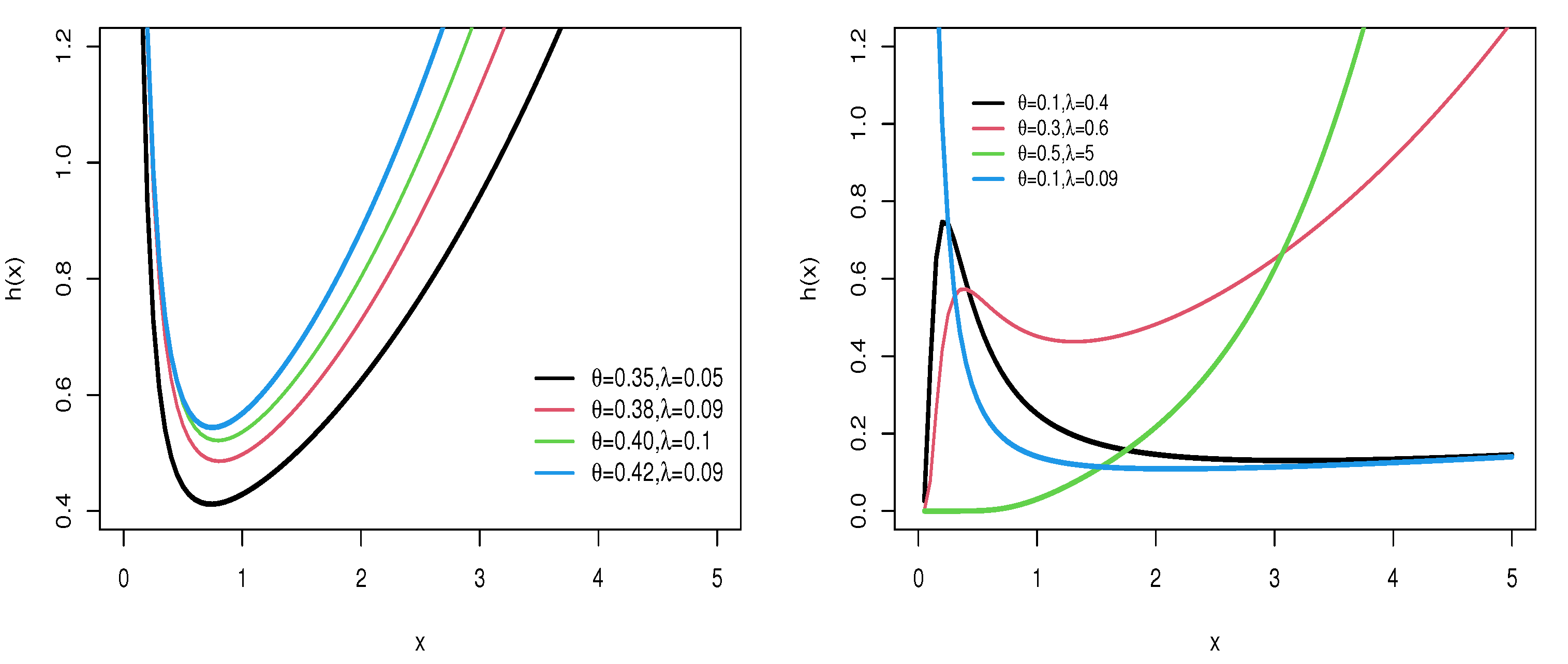
Figure 1 and Figure 2 provide visual representations of the density and hazard rate functions for varying parameter values. Figure 1 demonstrates that the density function $f\left(x\right)$ can exhibit symmetrical, right-skewed, left-skewed, or even bimodal forms. On the other hand, Figure 2 shows that the hazard rate function $h\left(x\right)$ can take on increasing, decreasing, or unimodal shapes depending on the parameter settings.

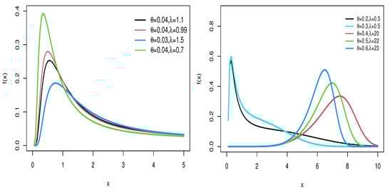
Figure 1. PDF of WFW distribution for several parameter settings.

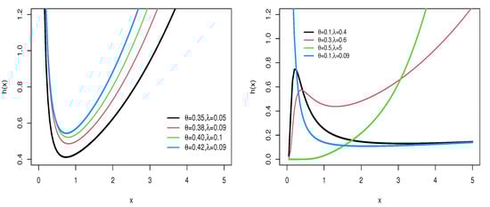
Figure 2. HRF of WFW distribution for several parameter settings.

The reversed hazard rate function of the WFW distribution is obtained as follows:

$$r(x:\theta ,\lambda )={\displaystyle \frac{2\left(\theta +\frac{\lambda }{x^2}\right)e^{-e^{\theta x-\frac{\lambda }{x}}+\theta x-\frac{\lambda }{x}}}{\left(1-exp\left(-e^{\theta x-\frac{\lambda }{x}}\right)\right)\left(1+exp\left(-e^{\theta x-\frac{\lambda }{x}}\right)\right)}}.$$

The inverse of the hazard function for the WFW distribution exhibits a decreasing trend across different parameter values. The quantile function is a widely used tool in data analysis and probability, providing valuable information about the distribution of data and their observed values. Let $Q\left(p\right)=F^{-1}\left(p\right)$ be the quantile function of X. Then, by solving a quadratic equation, the quantile function (for $0<p<1$) is obtained:

$$Q\left(p\right)={\displaystyle \frac{1}{2\theta }}\left\{log\left(-log\left({\displaystyle \frac{1-p}{1+p}}\right)\right)+\sqrt{{\left[log\left(-log\left({\displaystyle \frac{1-p}{1+p}}\right)\right)\right]}^2+4\theta \lambda }\right\}.$$

(3)

3. Properties

3.1. Asymptotic Properties

Let X be a random variable with parameters $\theta$ and $\lambda$. The asymptotic behavior of the CDF, PDF, and HRF are given by

$$F\left(x\right)\sim e^{-{\displaystyle \frac{\lambda }{x}}},f\left(x\right)\sim {\displaystyle \frac{\lambda }{x^2}}{e}^{-{\displaystyle \frac{\lambda }{x}}},h\left(x\right)\sim {\displaystyle \frac{\frac{\lambda }{x^2}{e}^{-\frac{\lambda }{x}}}{1-e^{-\frac{\lambda }{x}}}},$$

as $x\to 0^{+}$. When $x\to \infty$, the asymptotic behavior of these functions for the WFW distribution is expressed as

$$1-F\left(x\right)\sim 2e^{-e^{\theta x}},f\left(x\right)\sim 2\theta e^{\theta x}{e}^{-e^{\theta x}},h\left(x\right)\sim \theta e^{\theta x}.$$

3.2. Moments and Generating Function

Moments play crucial roles in identifying and quantifying various statistical characteristics, including detecting flattening and spacing, as well as assessing the coefficient of variation. In Table 1, the first four moments, standard deviation (SD), skewness (SK), and kurtosis (KR) are numerically computed. The rth moment of the WFW distribution can be determined using the following relationship [14]:

$$E\left(X^n\right)=n{\int }_0^{\infty }{x}^{n-1}[1-F\left(x\right)]dx.$$

Table 1. First four moments, standard deviation (SD), skewness (SK), and kurtosis (KR) for the WFW model.

	$\theta =0.04,\lambda =1.1$	$\theta =0.04,\lambda =0.99$	$\theta =0.04,\lambda =1.5$	$\theta =0.04,\lambda =0.5$
${\mu }_1^{\prime }$	10.923	10.773	11.439	10.040
${\mu }_2^{\prime }$	243.831	240.959	254.236	228.0944
${\mu }_3^{\prime }$	6860.908	6783.186	7146.237	6440.962
${\mu }_4^{\prime }$	219054.8	216538.5	228340.1	205525.1
$\mathrm{SD}$	11.15824	11.17569	11.106	11.282
$\mathrm{SK}$	1.063338	1.071	1.032	1.11053
$\mathrm{KR}$	3.29815	3.309	3.257	3.352
	$\theta =0.5,\lambda =20$	$\theta =0.5,\lambda =18$	$\theta =0.5,\lambda =26$	$\theta =0.5,\lambda =16$
${\mu }_1^{\prime }$	6.2996	5.980	7.174612	5.642
${\mu }_2^{\prime }$	40.71086	36.776	52.5268	32.84342
${\mu }_3^{\prime }$	268.776	231.495	391.2338	196.1263
${\mu }_4^{\prime }$	1807.249	1486.404	2957.79	1196.871
$\mathrm{SD}$	1.012774	1.0074	1.025543	1.001466
$\mathrm{SK}$	−0.5871091	−0.5543	−0.6650084	−0.5167628
$\mathrm{KR}$	3.301012	3.227	3.492299	3.147694
	$\theta =0.4,\lambda =20$	$\theta =0.3,\lambda =9$	$\theta =0.3,\lambda =14$	$\theta =0.3,\lambda =11$
${\mu }_1^{\prime }$	7.0534	5.565	6.869	6.119
${\mu }_2^{\prime }$	51.317	33.453	49.785	39.985
${\mu }_3^{\prime }$	383.059	213.284	376.477	274.881
${\mu }_4^{\prime }$	2922.048	1425.085	2947.551	1968.856
$\mathrm{SD}$	1.251	1.574	1.612	1.591
$\mathrm{SK}$	−0.516	−0.127	−0.294	0.20
$\mathrm{KR}$	3.147	2.603	2.776	2.672
	$\theta =1.5,\lambda =0.5$	$\theta =1.5,\lambda =1.0$	$\theta =1.5,\lambda =1.5$	$\theta =1.5,\lambda =2.0$
${\mu }_1^{\prime }$	0.631	0.849	1.022	1.169
${\mu }_2^{\prime }$	0.487	0.815	1.142	1.468
${\mu }_3^{\prime }$	0.430	0.854	1.364	1.947
${\mu }_4^{\prime }$	0.416	0.958	1.719	2.697
$\mathrm{SD}$	0.297	0.305	0.311	0.316
$\mathrm{SK}$	0.381	0.105	−0.055	−0.167
$\mathrm{KR}$	2.555	2.498	2.555	2.638

Employing the outcomes from the study conducted by [15], it is evident that

$$\begin{array}{ccc}\hfill E\left(X^n\right)& =& n{\int }_0^{\infty }{x}^{n-1}{\displaystyle \frac{2exp(-e^{\theta x-\frac{\lambda }{x}})}{1+exp(-e^{\theta x-\frac{\lambda }{x}})}}dx\hfill \\ & =& 2n\sum _{i=0}^{\infty }{(-1)}^i{\int }_0^{\infty }{x}^{n-1}{e}^{-(i+1)e^{\theta x-{\displaystyle \frac{\lambda }{x}}}}dx.\hfill \end{array}$$

Further, by using the result 3.471.9 of [16], the nth moment of the WFW distribution is

$$E\left(X^n\right)=2n\sum _{i=0}^{\infty }{\displaystyle \frac{{(-1)}^{i+j}{(i+1)}^j}{j!}}{\int }_0^{\infty }{x}^{n-1}{e}^{j\theta x-{\displaystyle \frac{j\lambda }{x}}}dx.$$

Then,

$$\begin{array}{cc}\hfill E\left(X^n\right)& =2n\sum _{i=0}^{\infty }{\displaystyle \frac{{(-1)}^{i+j}{(i+1)}^j}{j!}}\left[2{\left({\displaystyle \frac{j\lambda }{j\theta }}\right)}^{{\displaystyle \frac{n}{2}}}{K}_n\left(2\sqrt{j\theta j\lambda }\right)\right]\hfill \\ \hfill & =4n\left[{\left({\displaystyle \frac{\lambda }{\theta }}\right)}^{{\displaystyle \frac{n}{2}}}{K}_n\left(2j\sqrt{\theta \lambda }\right)\right]\sum _{i=0}^{\infty }{\displaystyle \frac{{(-1)}^{i+j}{(i+1)}^j}{j!}},\hfill \end{array}$$

(4)

where $v=n-1$ and

$$K_n\left(z\right)={\displaystyle \frac{\pi csc\left(\pi n\right)}{2}}[I_{-n}\left(z\right)-I_n\left(z\right)].$$

The modified Bessel function of the first kind is

$$I_n\left(x\right)=\sum _{m=0}^{\infty }{\displaystyle \frac{1}{\Gamma (m+m+1)m!}}{\left({\displaystyle \frac{x}{2}}\right)}^{2m+n},n\ne \mathbb{Z},$$

and $\Gamma \left(a\right)={\int }_0^{\infty }{x}^{a-1}{e}^{-x}dx$ denotes the gamma function. Similarly, the nth incomplete moment of X, say

$$E\left(X^n\right|X\le y)={\displaystyle \frac{1}{F\left(y\right)}}{\int }_0^y{x}^{n}f\left(x\right)dx,$$

is

$$\begin{array}{cc}\hfill E\left(X^n\right|X\le y)& ={\displaystyle \frac{1}{F\left(y\right)}}{\int }_0^{\infty }{x}^n{\displaystyle \frac{2(\theta +\frac{\lambda }{x^2})e^{\theta x-\frac{\lambda }{x}}exp(-e^{\theta x-\frac{\lambda }{x}})}{{(1+exp(-e^{\theta x-\frac{\lambda }{x}}))}^2}}dx\hfill \\ \hfill & ={\displaystyle \frac{2}{F\left(y\right)}}\sum _{i=0}^{\infty }{(-1)}^i(i+1){\int }_0^{\infty }{x}^n(\theta +{\displaystyle \frac{\lambda }{x^2}})e^{\theta x-{\displaystyle \frac{\lambda }{x}}}{e}^{-(i+1)e^{\theta x-{\displaystyle \frac{\lambda }{x}}}}dx\hfill \\ \hfill & ={\displaystyle \frac{2}{F\left(y\right)}}\sum _{i,j=0}^{\infty }{\displaystyle \frac{{(-1)}^{i+j}{(i+1)}^{j+1}}{j!}}{\int }_0^{\infty }{x}^n(\theta +{\displaystyle \frac{\lambda }{x^2}})e^{(j+1)\theta x-{\displaystyle \frac{(j+1)\lambda }{x}}}dx.\hfill \end{array}$$

Following Theorem 2 of [17], then

$$\begin{array}{cc}\hfill E\left(X^n\right|X\le y)& ={\displaystyle \frac{2}{F\left(y\right)}}\sum _{i,j=0}^{\infty }{\displaystyle \frac{{(-1)}^{i+j}{(i+1)}^{j+1}}{j!}}\hfill \\ \hfill & \times \left\{\theta \gamma \left(n+1,(j+1)\theta y-{\displaystyle \frac{(j+1)\lambda }{y}}\right)+\lambda \gamma \left(n-1,{\displaystyle \frac{(j+1)\lambda }{y}}\right)\right\},\hfill \end{array}$$

(5)

for $n\ge 1$, where

$$\gamma (a,x)={\int }_0^x{t}^{a-1}{e}^{-t}dt$$

represents the lower incomplete gamma function.

3.3. Moment Generating Function

For a random variable X, the moment generating function (MGF) is given by

$$M_X\left(t\right)\equiv {\int }_0^{\infty }{e}^{tx}f\left(x\right)dx=\sum _{j=0}^{\infty }{\displaystyle \frac{t^k}{k!}}E\left(X^n\right).$$

Based on (4), the MGF of X can be expressed as

$$M_X\left(t\right)=4n\sum _{j=0}^{\infty }\sum _{i=0}^{\infty }{\displaystyle \frac{{(-1)}^{i+j}{(i+1)}^j{t}^k}{j!k!}}\left[{\left({\displaystyle \frac{\lambda }{\theta }}\right)}^{{\displaystyle \frac{n}{2}}}{K}_n\left(2j\sqrt{\theta \lambda }\right)\right].$$

4. Entropy

4.1. Cumulative Entropy

Cumulative entropy serves as a measure for quantifying the uncertainty of a random variable. It is defined based on the CDF of the random variable X [18]. Then, the cumulative entropy is defined as:

$$CE\left(X\right)=-{\int }_{-\infty }^{\infty }F\left(x\right)log\left(F\left(x\right)\right)dx.$$

By (1), the $CE\left(X\right)$ can be expressed as

$$\begin{array}{cc}\hfill CE\left(X\right)& =-{\int }_0^{\infty }{\displaystyle \frac{1-exp\left(-e^{\theta x-\frac{\lambda }{x}}\right)}{1+exp\left(-e^{\theta x-\frac{\lambda }{x}}\right)}}log\left({\displaystyle \frac{1-exp\left(-e^{\theta x-\frac{\lambda }{x}}\right)}{1+exp\left(-e^{\theta x-\frac{\lambda }{x}}\right)}}\right)dx\hfill \\ \hfill & =-{\int }_0^{\infty }{\displaystyle \frac{1-exp\left(-e^{\theta x-\frac{\lambda }{x}}\right)}{1+exp\left(-e^{\theta x-\frac{\lambda }{x}}\right)}}\left(log\left(1-exp\left(-e^{\theta x-{\displaystyle \frac{\lambda }{x}}}\right)\right)-log\left(1+exp\left(-e^{\theta x-{\displaystyle \frac{\lambda }{x}}}\right)\right)\right)dx.\hfill \end{array}$$

Using the Taylor expansion, the cumulative entropy of the flexible Weibull weighted distribution is

$$\begin{array}{cc}\hfill CE\left(X\right)=& =\sum _{i,j=0}^{\infty }{\displaystyle \frac{{(-1)}^i[1+{(-1)}^{i+1}]}{i+1}}\left\{e^{(i+j+1)e^{\theta x-{\displaystyle \frac{\lambda }{x}}}}-e^{-(i+j+2)e^{\theta x-{\displaystyle \frac{\lambda }{x}}}}\right\}\hfill \\ \hfill & =\sum _{i,j=0}^{\infty }{\displaystyle \frac{{(-1)}^i[1+{(-1)}^{i+1}]}{i+1}}{\int }_0^{\infty }{e}^{-(2i+2j+3)e^{\theta x-{\displaystyle \frac{\lambda }{x}}}}dx\hfill \\ \hfill & =\sum _{i,j=0}^{\infty }{\displaystyle \frac{{(-1)}^i[1+{(-1)}^{i+1}]}{i+1}}{\int }_0^{\infty }{e}^{-k{e}^{\theta x-{\displaystyle \frac{\lambda }{x}}}}dx\hfill \\ \hfill & =\sum _{l=0}^{\infty }{\displaystyle \frac{{(-1)}^l}{l!}}{k}^l\sum _{i,j=0}^{\infty }{\displaystyle \frac{{(-1)}^i+l[1+{(-1)}^{i+1}]k^l}{l!,i+1}}{\int }_0^{\infty }{e}^{l\theta x-{\displaystyle \frac{l\lambda }{x}}}dx.\hfill \end{array}$$

Based on [14], it can be seen that

$${\int }_0^{\infty }{e}^{-\gamma x-{\displaystyle \frac{\lambda }{4x}}}dx=\sqrt{{\displaystyle \frac{\lambda }{\gamma }}}{K}_1\left(\sqrt{\gamma \lambda }\right)$$

and

$$CE\left(X\right)=\sum _{i,j=0}^{\infty }{\displaystyle \frac{{(-1)}^i[1+{(-1)}^{i+1}]}{i+1}}\sum _0^{\infty }{\displaystyle \frac{{(-1)}^l}{l!}}{k}^l\left[\sqrt{{\displaystyle \frac{\lambda }{l\theta }}}{K}_1\left(\sqrt{4l\theta \lambda }\right)\right].$$

4.2. Cumulative Residual Entropy

Cumulative residual entropy [19,20] is a metric for measuring uncertainty in the time remaining until an event occurs. This concept considered the survival and hazard distributions and provides a better description of temporal unpredictability in events. The applications of cumulative residual entropy has been studied in various fields, including insurance and risk assessment [21]. For a random variable X, the cumulative residual entropy is given by

$$CRE\left(X\right)=-{\int }_0^{\infty }(1-F\left(x\right))log(1-F\left(x\right))dx.$$

By using the equation above, the $CRE\left(X\right)$ can be expanded as

$$\begin{array}{cc}\hfill CRE\left(X\right)& ={\int }_0^{\infty }(1-F\left(x\right))\sum _{i=0}^{\infty }{\displaystyle \frac{F{\left(x\right)}^{i+1}}{i+1}}dx\hfill \\ \hfill & =-{\int }_0^{\infty }{\displaystyle \frac{2e^{-H\left(x\right)}}{1+e^{-H\left(x\right)}}}log\left({\displaystyle \frac{2e^{-H\left(x\right)}}{1+e^{-H\left(x\right)}}}\right)dx\hfill \\ \hfill & =-{\int }_0^{\infty }{\displaystyle \frac{2e^{-H\left(x\right)}}{1+e^{-H\left(x\right)}}}\left[log2+H\left(x\right)-log(1+e^{-H\left(x\right)})\right]dx\hfill \\ \hfill & =-{\int }_0^{\infty }{\displaystyle \frac{2e^{-H\left(x\right)}}{1+e^{-H\left(x\right)}}}\left[log2+H\left(x\right)\right]dx+{\displaystyle \frac{2e^{-H\left(x\right)}}{1+e^{-H\left(x\right)}}}\sum _{i=0}^{\infty }{\displaystyle \frac{{(-1)}^i{e}^{-(i+1)H\left(x\right)}}{(i+1)(1+e^{-H\left(x\right)})}}dx\hfill \\ \hfill & =-2log2\sum _{i,j=0}^{\infty }{\displaystyle \frac{{(-1)}^{i+j}{(i+1)}^j}{j!}}{e}^{\theta jx-{\displaystyle \frac{j\lambda }{x}}}-2\sum _{i,j=0}^{\infty }{\displaystyle \frac{{(-1)}^{i+j}{(i+1)}^j}{j!}}{\int }_0^{\infty }{e}^{2[\theta jx-{\displaystyle \frac{j\lambda }{x}}]}dx\hfill \\ \hfill & +2\sum _{i,j=0}^{\infty }{\displaystyle \frac{{(-1)}^{i+j+k}{(i+1)}^j{(i+j+1)}^k}{j!,k!}}{\int }_0^{\infty }{e}^{k\theta x-{\displaystyle \frac{k\lambda }{x}}}dx.\hfill \end{array}$$

Finally, based on [14], the $CRE\left(X\right)$ can be expanded as

$$CRE\left(X\right)=2\sum _{i,j=0}^{\infty }{\displaystyle \frac{{(-1)}^{i+j+k}{(i+1)}^j{(i+j+1)}^k}{j!,k!}}\left\{\sqrt{{\displaystyle \frac{\lambda }{\theta }}}{K}_1\left(k\sqrt{\theta \lambda }\right)\right\}.$$

4.3. Rényi Entropy

For a random variable X, the Rényi entropy [22] is given by

$$I_n\left(\delta \right)={\displaystyle \frac{1}{1-\delta }}log\left({\int }_0^{\infty }f{\left(x\right)}^{\delta }dx\right).$$

(6)

Additional properties of Rényi entropy can be seen in [23]. Using (6), the term $f{\left(x\right)}^{\delta }$ can be expressed as

$$f{\left(x\right)}^{\delta }={\displaystyle \frac{2^{\delta }{(\theta -\frac{\lambda }{x^2})}^{\delta }}{{[1+e^{H\left(x\right)}]}^{2\delta }}}H{\left(x\right)}^{\delta }{e}^{\delta H\left(x\right)},$$

where

$$I_n\left(\delta \right)={\displaystyle \frac{1}{1-\delta }}log\left({\int }_0^{\infty }{2}^{\delta }{\displaystyle \frac{{(\theta -\frac{\lambda }{x^2})}^{\delta }}{{[1+e^{H\left(x\right)}]}^{2\delta }}}H{\left(x\right)}^{\delta }{e}^{\delta H\left(x\right)}dx\right).$$

Note that

$${\displaystyle \frac{1}{{[1+e^{H\left(x\right)}]}^{2\delta }}}=\sum _{i=0}^{\infty }\left({\displaystyle \genfrac{}{}{0pt}{}{-2\delta }{i}}\right)e^{iH\left(x\right)}.$$

Thus,

$$\begin{array}{cc}\hfill {\int }_0^{\infty }f{\left(x\right)}^{\delta }dx& =2^{\delta }\sum _{i=0}^{\infty }\left({\displaystyle \genfrac{}{}{0pt}{}{-2\delta }{i}}\right){(\theta +{\displaystyle \frac{\lambda }{x^2}})}^{\delta }H{\left(x\right)}^{\delta }{e}^{-(i+\delta )H\left(x\right)}\hfill \\ \hfill & =\sum _{i,j=0}^{\infty }\left({\displaystyle \genfrac{}{}{0pt}{}{-2j}{i}}\right)\left({\displaystyle \genfrac{}{}{0pt}{}{\delta }{j}}\right)2^{\delta }{\theta }^{\delta -j}{\lambda }^j\ast {\int }_0^{\infty }{x}^{-2j}H{\left(x\right)}^{\delta }{e}^{-(i+\delta )H\left(x\right)}dx\hfill \\ \hfill & =\sum _{k=0}^{\infty }\sum _{i,j=0}^{\infty }\left({\displaystyle \genfrac{}{}{0pt}{}{-2j}{i}}\right)\left({\displaystyle \genfrac{}{}{0pt}{}{\delta }{j}}\right)2^{\delta }{\theta }^{\delta -j}{\lambda }^j{\int }_0^{\infty }{x}^{-2j}{e}^{\theta (\delta -k)x-{\displaystyle \frac{(\delta +k)\lambda }{x}}}dx.\hfill \end{array}$$

Based on Formula (3.471 9) of [16], $I_n\left(\delta \right)$ can be simplified as

$$\begin{array}{cc}\hfill I_n\left(\delta \right)& ={\displaystyle \frac{1}{1-\delta }}\left\{\delta log\left(2\right)+\sum _{i=0,j=0,k=0}^{\infty }\left(log\left(M\right(i,j,k)\right)\right.\hfill \\ \hfill & \left.\times \left[2{\left({\displaystyle \frac{(\delta +k)\beta }{\theta (k-\delta )}}\right)}^{{\displaystyle \frac{1-2j}{2}}}{K}_{(1-2j)}\left(2\sqrt{(\delta +k)\lambda (\delta -k)\theta }\right)\right]\right\},\hfill \end{array}$$

where

$$M(i,i,k)=\left({\displaystyle \genfrac{}{}{0pt}{}{-2j}{i}}\right)\left({\displaystyle \genfrac{}{}{0pt}{}{\delta }{j}}\right){\theta }^{\delta -j}{\lambda }^j.$$

5. Estimation Methods

5.1. Maximum Likelihood Estimation Method

The parameters of the WFW distribution are estimated using the MLE method. Given a set of random samples, $x_1,x_2,\dots ,x_n$, following the WFW distribution, the likelihood function is derived. Using (2), the $L\left(x\right)$ can be expressed as

$$\begin{array}{cc}\hfill L\left(x\right)& =\prod _{i=1}^n{\displaystyle \frac{2\left(\theta +\frac{\lambda }{x_i^2}\right)e^{\theta x_i-\frac{\lambda }{x_i}}exp\left(-e^{\theta x_i-\frac{\lambda }{x_i}}\right)}{{\left[1+exp\left(-e^{\theta x_i-\frac{\lambda }{x_i}}\right)\right]}^2}}\hfill \\ \hfill & =2^n{\displaystyle \frac{{\prod }_{i=1}^n\left(\theta +\frac{\lambda }{x_i^2}\right)exp\left(-{\sum }_{i=1}^n{e}^{\theta x_i-\frac{\lambda }{x_i}}\right)}{{\prod }_{i=1}^n{\left(1+e^{-e^{\theta x_i-\frac{\lambda }{x_i}}}\right)}^2}}{e}^{\theta {\sum }_{i=1}^n{x}_i-{\sum }_{i=1}^n{\displaystyle \frac{\lambda }{x_i}}}\hfill \end{array}$$

By taking the natural logarithm, the log-likelihood function is obtained as

$$\ell \left(\alpha \right)=nlog\left(2\right)+{\displaystyle \frac{{\sum }_{i=1}^{n}log\left(\theta +\frac{\lambda }{{x_i}^2}\right)+\theta {\sum }_{i=1}^n{x}_i-{\sum }_{i=1}^n\frac{\lambda }{x_i}-{\sum }_{i=1}^n{e}^{(\theta x_i-\frac{\lambda }{x_i})}}{2n{\sum }_{i=1}^{n}log(1+e^{-e^{\theta x_i-\frac{\lambda }{x_i}}})}}.$$

MLEs are numerically calculated using caret package [24] of R software [25].

5.2. Least Squares Estimation Method

The least squares estimation (LSE) approach seeks optimal model parameters to minimize the sum of the square difference between the observed data points and those predicted by the model. For a model defined by $\alpha$ and $\beta$ parameters and a distribution F, the LSE method defines the objective function:

$$S_{LSE}(\theta ,\lambda )=\sum _{i=1}^n{\left(F\left(x_{i:n}\right)-{\displaystyle \frac{i}{n+1}}\right)}^2,$$

where $x_{1:n},x_{2:n},\dots ,x_{n:n}$ are ordered samples from the data and $F\left(x_{i:n}\right)$ represents the value of the hypothetical distribution at $x_{i:n}$.

5.3. Weighted Least Squares Estimation

In the weighted LSE method, the objective function is

$$S_{WLSE}(\theta ,\lambda )=\sum _{i=1}^n(n+2){\displaystyle \frac{{(n+1)}^2}{i(n-i+1)}}{\left[F\left(x_{i:n}\right)-{\displaystyle \frac{i}{n+1}}\right]}^2,$$

(7)

where $x_{1:n},x_{2:n},\dots ,x_{n:n}$ represents the ordered samples from the data, and $F\left(x_{i:n}\right)$ denotes the value of the hypothetical distribution at $x_{i:n}$.

5.4. Cramer–Von Mises Estimator

The Cramer–von Mises estimator (CME) is defined as

$$S_{CME}(\theta ,\lambda )={\displaystyle \frac{1}{12n}}+\sum _{i=1}^n{\left[F\left(x_{i:n}\right)-{\displaystyle \frac{2i-1}{2n}}\right]}^2,$$

(8)

where $x_{1:n},x_{2:n},\dots ,x_{n:n}$ represents the ordered samples from the data, and $F\left(x_{i:n}\right)$ denotes the value of the hypothetical distribution at $x_{i:n}$.

5.5. Anderson–Darling Estimator

The Anderson–Darling estimator (ADE) and right-tailed Anderson–Darling estimator (RTADE) are respectively defined as

$$\begin{array}{cc}\hfill S_{ADE}(\theta ,\lambda )& =-n-{\displaystyle \frac{1}{n}}\sum _{i=1}^n(2i-1)\left[logF\left(x_i\right)+log\overline{F}\left(x_{n+1-i}\right)\right]\hfill \end{array}$$

(9)

$$\begin{array}{cc}\hfill S_{RTADE}(\theta ,\lambda )& ={\displaystyle \frac{n}{2}}-2\sum _{i=1}^{n}F\left(x_i\right)-{\displaystyle \frac{1}{n}}\sum _{i=1}^n(2i-1)log\overline{F}\left(x_{n+1-i}\right),\hfill \end{array}$$

(10)

where $\overline{F}(.)=1-F(.)$. In these equations, $x_1,x_2,\dots ,x_n$ represents the samples from the data, and $F\left(x_i\right)$ denotes the value of the hypothetical distribution at $x_i$. The estimation of each parameter can therefore be obtained when the first partial derivative of the log-likelihood function for each of the parameters is taken, equated to zero, and solved simultaneously. Note that the solution cannot be obtained in closed form, but it can be obtained by solving numerically using the R software [25].

6. Simulations

In the study of the estimation and comparison of different estimation methods, several simulations were conducted to compare the methods for estimating the parameters $\theta$ and $\lambda$ of the WFW distribution with generating $N=1000$ Monte Carlo replicates for the WFW model based on Equation (3) with sample sizes $n=50,100,300,500$. The simulations were performed under the following parameter settings: $(\theta ,\lambda )=(0.5,1)$ and $(\theta ,\lambda )=(1,1)$. To assess the accuracy of the estimation methods, the Bias and MSE were calculated using the following equations:

$$\begin{array}{cc}\hfill \mathrm{Bias}\left(\widehat{\alpha }\right)& ={\displaystyle \frac{1}{N}}\sum _{i=1}^N({\widehat{\theta }}_i-\theta ),\mathrm{Bias}\left(\widehat{\lambda }\right)={\displaystyle \frac{1}{N}}\sum _{i=1}^N({\widehat{\lambda }}_i-\lambda ),\hfill \\ \hfill \mathrm{MSE}\left(\theta \right)& ={\displaystyle \frac{1}{N}}\sum _{i=1}^N{({\widehat{\theta }}_i-\theta )}^2,\mathrm{MSE}\left(\lambda \right)={\displaystyle \frac{1}{N}}\sum _{i=1}^N{({\widehat{\lambda }}_i-\lambda )}^2.\hfill \end{array}$$

This section discusses the assessment of estimating the $\theta$ and $\lambda$ parameters and concerning bias and root mean square error MSE values. Furthermore, the analysis of bias was conducted. The bias value reflects the estimation method accuracy by averaging the possible deviation of estimates from the true parameter value. The MSE was used as well. This value sums up variance and bias for a deep comparison, where a smaller value is considered as a more accurate estimator. It can be seen in Table 2 that, when sample size n increases, the size of the bias decreases for all methods, which shows an improvement in accuracy. In this table, ADE and RTADE methods have a better performance of $\theta$ estimation than other methods. Also, the MLE method is more biased in smaller samples, but reduces its bias as the sample size increases. In Table 3, the value of MSE in all methods indicates the improvement of estimates in large samples sizes, where the RTADE method has the lowest values of MSE compared to other methods. Also, the MLE and CME methods have higher MSE in small samples, but both improve with increasing sample size. Based on the results, it is suggested to use ADE and RTADE methods to estimate model parameters, because in many cases these methods have lower bias and MSE values than other methods. Also, in small samples, WLSE can be a suitable option. The performance of the MLE method can improved with larger sample size.

Table 2. Bias and RMSE of $\alpha$ and $\beta$ for different sample sizes n.

Bias for $\theta =1$	n	MLEs	LSEs	WLSEs	CMEs	ADEs	RTADEs
	20	0.0707	0.0039	0.0129	0.0812	0.0255	0.0440
	50	0.0256	0.0013	0.0077	0.0304	0.0099	0.0169
	100	0.0099	−0.0020	0.0028	0.0122	0.0028	0.0052
	200	0.0050	−0.0014	0.0010	0.0057	0.0009	0.0008
	500	0.0024	0.0006	0.0016	0.0035	0.0012	0.0016
Bias for $\lambda =1$	n	MLEs	LSEs	WLSEs	CMEs	ADEs	RTADEs
	20	0.1061	0.0202	0.0311	0.1116	0.0444	0.0839
	50	0.0396	0.0101	0.0178	0.0445	0.0190	0.0343
	100	0.0174	0.0011	0.0073	0.0179	0.0066	0.0122
	200	0.0061	−0.0039	−0.0003	0.0044	−0.0008	−0.0004
	500	0.0027	0.0000	0.0013	0.0033	0.0006	0.0016
MSE for $\theta =1$	n	MLEs	LSEs	WLSEs	CMEs	ADEs	RTADEs
	20	0.1948	0.2158	0.2010	0.2538	0.1827	0.1958
	50	0.1045	0.1258	0.1145	0.1342	0.1087	0.1115
	100	0.0661	0.0841	0.0751	0.0866	0.0725	0.0749
	200	0.0474	0.0589	0.0528	0.0597	0.0517	0.0532
	500	0.0288	0.0379	0.0326	0.0382	0.0323	0.0326
MSE for $\lambda =1$	n	MLEs	LSEs	WLSEs	CMEs	ADEs	RTADEs
	20	0.3333	0.3366	0.3248	0.3865	0.3087	0.3622
	50	0.1778	0.2027	0.1898	0.2146	0.1835	0.2102
	100	0.1268	0.1452	0.1358	0.1489	0.1334	0.1513
	200	0.0838	0.0964	0.0895	0.0973	0.0888	0.0989
	500	0.0509	0.0598	0.0546	0.0601	0.0543	0.0608

Table 3. MSE and Bias for $\theta$ and $\lambda$ with n samples.

Bias for $\theta =0.5$	n	MLEs	LSEs	WLSEs	CMEs	ADEs	RTADEs
	20	0.03848	0.01386	0.01524	0.05298	0.01992	0.02619
	50	0.01225	−0.00096	0.00260	0.01317	0.00367	0.00728
	100	0.00644	0.00041	0.00234	0.00738	0.00261	0.00440
	200	0.00465	0.00161	0.00267	0.00507	0.00262	0.00313
	500	0.00070	−0.00075	−0.00008	0.00062	−0.00026	0.00003
Bias for $\lambda =1$	n	MLEs	LSEs	WLSEs	CMEs	ADEs	RTADEs
	20	0.11110	0.03352	0.03706	0.13005	0.05047	0.09532
	50	0.03963	0.00562	0.01467	0.04093	0.01528	0.03732
	100	0.02875	0.01374	0.01831	0.03127	0.01813	0.02871
	200	0.01243	0.00486	0.00786	0.01346	0.00739	0.01084
	500	0.00199	−0.00221	−0.00043	0.00119	−0.00115	0.00058
MSE for $\theta =0.5$	n	MLEs	LSEs	WLSEs	CMEs	ADEs	RTADEs
	20	0.09613	0.11221	0.10429	0.13553	0.09246	0.09473
	50	0.05239	0.06250	0.05693	0.06627	0.05443	0.05605
	100	0.03401	0.04156	0.03730	0.04300	0.03626	0.03730
	200	0.02483	0.02923	0.02625	0.02989	0.02604	0.02644
	500	0.01552	0.01908	0.01687	0.01915	0.01676	0.01702
MSE for $\lambda =1$	n	MLEs	LSEs	WLSEs	CMEs	ADEs	RTADEs
	20	0.36420	0.37965	0.36290	0.43784	0.34708	0.43814
	50	0.19811	0.22821	0.21303	0.24043	0.20657	0.25621
	100	0.14033	0.16054	0.15059	0.16596	0.14732	0.17763
	200	0.09688	0.10939	0.10210	0.11110	0.10170	0.11767
	500	0.05945	0.07042	0.06431	0.07066	0.06398	0.07407

7. Risk Indicators

7.1. The Mean of Order P and Optimal Order of P

The ${\mathrm{MOP}}_{\left[P\right]}$ analysis [26], formally defined by [27], is used to characterize the central tendency or average behavior of a dataset based on different orders of moments. The ${\mathrm{MOP}}_{\left[P\right]}$ is calculated by raising each data point to the power of P (a positive integer) and then taking the average of these values. The optimal order of P in ${\mathrm{MOP}}_{\left[P\right]}$ analysis refers to determining the most suitable value of P that provides meaningful insights into the dataset’s characteristics or distribution. The choice of P can influence the sensitivity of the analysis to different aspects of the dataset. This is usually done by calculating ${\mathrm{MOP}}_{\left[P\right]}$ for different p values (e.g., $p=1,2,3,\dots$) to examine how much influence the dataset has on different moments.

7.2. The PORT-VaR Estimator

The PORT-VaR estimator is a statistical method used for risk analysis and extreme value modeling. This method is particularly useful for identifying and analyzing extreme events or peaks in a dataset that exceed a specified threshold, which is often determined based on a certain level of confidence or risk tolerance. The PORT-VaR estimator calculates the value-at-risk (VaR) associated with the chosen threshold. VaR represents the maximum potential loss that could occur within a given confidence interval (e.g., 95% or 99%) under normal market conditions. The PORT-VaR estimator is widely used in modeling and analyzing rare events or outliers, which may have significant implications for risk assessment and mitigation strategies. It helps in understanding the probability and severity of extreme events, thereby enabling organizations to prepare and respond effectively to potential risks; see [28] for more details.

The necessary steps to obtain the PORT-VaR estimator are as follows:

• Gather relevant data that capture extreme events or rare occurrences. Clean and preprocess the data to ensure quality and suitability for analysis.
• Choose an appropriate statistical model.
• Select a threshold above which extreme events are considered for analysis. This threshold is crucial and should be based on domain expertise and risk management goals.
• Identify all data points that exceed the chosen threshold to form the PORT subset.
• Estimate the VaR for each peak in the PORT subset, where VaR represents the maximum expected loss at a specified confidence level based on extreme value modeling.
• Analyze the distribution of PORT-VaR estimates to quantify the tail risk associated with extreme events. Assess the impact of these events on overall risk exposure.
• Utilize PORT-VaR results to inform risk management strategies, such as setting reserves, determining insurance premiums, or implementing risk mitigation measures.

8. Applications

This section presents and evaluates three different applications of the proposed model. Each application demonstrates the model’s effectiveness in capturing the underlying patterns within the data. Furthermore, we assess its performance by comparing it against other well-established distributions, highlighting its advantages and potential limitations in various scenarios. Through this comparative analysis, we aim to provide a comprehensive understanding of the model’s strengths and its applicability across different datasets, such as the exponentiated Weibull (EW) [29], modified Weibull (MW) [30], beta Weibull (BW) [3], gamma flexible Weibull (GFW) [31], and Kumaraswamy Burr XII (KwBXII) [32]. The best-fitting model is identified based on the Cramer–von Mises statistic (${\mathbf{W}}^{\ast }$), Anderson–Darling statistic (${\mathbf{A}}^{\ast }$), Akaike information criterion (AIC), consistent Akaike information criterion (CAIC), Bayesian information criterion (BIC), and Hannan–Quinn information criterion (HQIC). The MLEs, standard errors (SEs), and relevant statistics are computed using the AdequacyModel package [33] in R software [25].

8.1. Failure Times Dataset

The failure times of 50 components (measured per 1000 h) are given in [34], as follows: 0.036, 0.058, 0.061, 0.074, 0.078, 0.086, 0.102, 0.103, 0.114, 0.116, 0.148, 0.183, 0.192, 0.254, 0.262, 0.379, 0.381, 0.538, 0.570, 0.574, 0.590, 0.618, 0.645, 0.961, 1.228, 1.600, 2.006, 2.054, 2.804, 3.058, 3.076, 3.147, 3.625, 3.704, 3.931, 4.073, 4.393, 4.534, 4.893, 6.274, 6.816, 7.896, 7.904, 8.022, 9.337, 10.940, 11.020, 13.880, 14.730, 15.080. These failure time datasets are used to analyze the failure behavior of components, fit probabilistic models for reliability analysis, and predict the lifespan of components. Table 4 shows the MLEs and their respective standard errors (SEs) for the parameters of different models fitted to the failure time data. From this table, parameter estimates from the WFW model are shown to have relatively small standard error estimates, indicating a good fit for the model to the actual data. On the other hand, estimates from models like MW, EW, and BW result in higher standard errors, suggesting a potential compromise in parameter estimation accuracy. More goodness-of-fit statistics (the measurements are considered test statistics, both $W^{\ast }$ and $A^{\ast }$) and model selection criteria (AIC, CAIC, BIC, and HQIC) are summarized in Table 5. Smaller values for these metrics are reflective of a better model fit. As can be seen, the WFW model has the lowest results on all criteria, proving its superiority over competing models. In particular, the value of AIC is equal to 192.294 in the WFW model, and this value is lower than that of the other models, demonstrating that the WFW model is more accurate in generalizing the data. The WWF model aligns the closest with the blue circles (empirical distribution), supporting the goodness of the WFW model in terms of fitting to the real failure time data. Thus, the results of this study support the ability of the WFW model to adequately analyze and predict actual real failure time data.

Table 4. MLEs and their respective SEs of fitted models for failure time dataset.

Model			MLE (SE)
WFW$(\theta ,\lambda )$	0.109	0.146
	$\left(0.011\right)$	$\left(0.03\right)$
GFW$(a,\theta ,\lambda )$	1.362	0.109	0.126
	$\left(0.19\right)$	$\left(0.013\right)$	$\left(0.033\right)$
FW$(\alpha ,\beta )$	0.099	0.183
	$\left(0.012\right)$	$\left(0.034\right)$
MW$(\alpha ,\lambda ,\beta )$	0.496	0.034	0.562
	$\left(0.099\right)$	$\left(0.025\right)$	$\left(0.098\right)$
EW$(\alpha ,\lambda ,\beta )$	0.290	0.770	0.785
	$\left(0.681\right)$	$\left(0.99\right)$	$\left(1.546\right)$
KwBXII$(a,b,c,k,s)$	0.121	2.199	4.381	1.193	21.015
	$\left(0.019\right)$	$\left(0.477\right)$	$\left(0.147\right)$	$\left(0.217\right)$	$\left(0.125\right)$
BW$(a,b,\alpha ,\beta )$	0.708	0.703	0.412	0.819
	$\left(1.392\right)$	$\left(1.46\right)$	$\left(1.575\right)$	$\left(1.057\right)$

Table 5. Evaluation metrics for the models applied to failure time dataset.

Model	${\mathit{W}}^{\ast }$	${\mathit{A}}^{\ast }$	AIC	CAIC	BIC	HQIC
WFW$(\theta ,\lambda )$	0.041	0.267	192.294	192.55	196.118	193.750
GFW$(a,\alpha ,\beta )$	0.042	0.257	193.850	194.372	199.586	196.035
FW$(\alpha ,\beta )$	0.079	0.414	195.846	196.101	199.670	197.302
MW$(\alpha ,\lambda ,\beta )$	0.130	0.850	208.727	209.249	214.463	210.912
EW$(\alpha ,\lambda ,\beta )$	0.150	0.946	210.713	211.234	216.449	212.897
BW$(a,b,\alpha ,\beta )$	0.149	0.942	212.696	213.585	220.344	215.608
KwBXII$(a,b,c,k,s)$	1.132	0.870	213.086	214.450	222.646	216.726

8.2. COVID-19 Mortality Dataset

The dataset includes the number of COVID-19 deaths recorded across 83 counties in Illinois, United States, up to December 2021. The reported number of deaths are as follows: 169, 13, 28, 91, 13, 107, 4, 41, 31, 89, 46, 57, 108, 146, 35, 30, 32, 156, 38, 52, 21, 113, 73, 59, 130, 93, 10, 40, 101, 25, 36, 16, 15, 95, 90, 101, 21, 150, 57, 32, 34, 127, 184, 38, 69, 115, 78, 121, 165, 24, 53, 58, 72, 15, 38, 108, 85, 104, 39, 110, 82, 16, 58, 7, 15, 7, 107, 67, 74, 14, 8, 56, 29, 124, 52, 19, 72, 30, 66, 34, 196, 201, 98. This dataset can be found at: https://data.world/associatedpress/johns-hopkins-coronavirus-case-tracker (accessed on 16 February 2025).

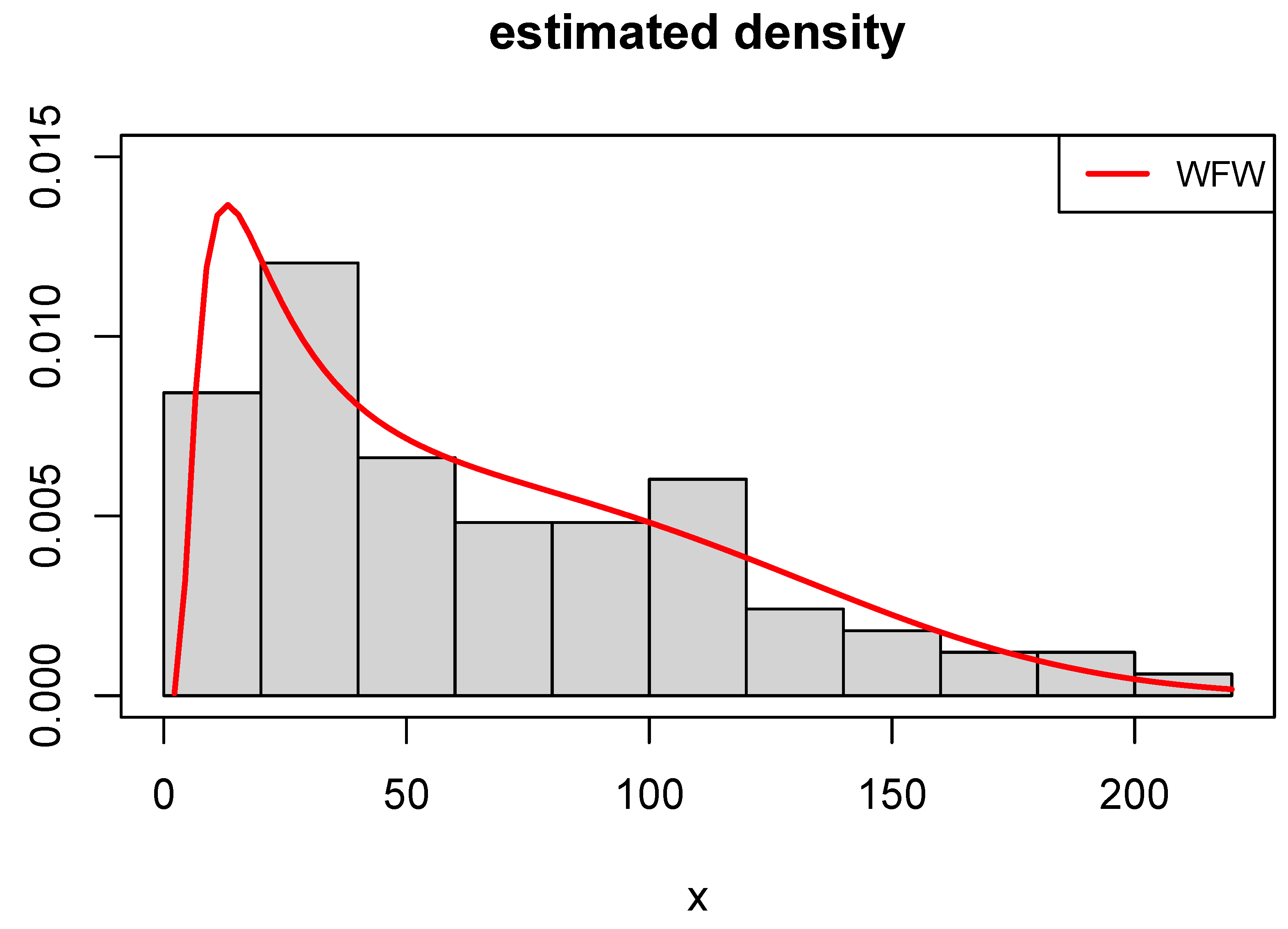
The obtained results regarding MLEs and their associated SEs are presented in Table 6. The results indicate that the WFW, GFW, and FW models yield precise parameter estimates with relatively low SEs, while other models exhibit higher SEs. Table 7 reports the values of various model selection criteria, showing that the WFW model consistently achieves the lowest values. Consequently, it is identified as the most suitable model for the data. Figure 3 illustrates the estimated density functions for the top-performing models. Among them, the WFW model demonstrates the closest agreement with the empirical histogram, underscoring its suitability for modeling the observed data.

Table 6. Findings from the fitted models to COVID-19 mortality dataset.

Model			MLE (SE)
WFW$(\theta ,\lambda )$	0.010	23.243
	$\left(0.0006\right)$	$\left(3.755\right)$
GFW$(a,\alpha ,\beta )$	1.702	0.010	14.005
	$\left(0.253\right)$	$\left(0.001\right)$	$\left(4.458\right)$
FW$(\alpha ,\beta )$	0.008	32.812
	$\left(0.001\right)$	$\left(4.290\right)$
MW$(\alpha ,\lambda ,\beta )$	0.005	0.003	1.161
	$\left(0.002\right)$	$\left(0.002\right)$	$\left(0.116\right)$
EW$(\alpha ,\lambda ,\beta )$	0.013	1.418	0.986
	$\left(0.005\right)$	$\left(0.503\right)$	$\left(0.574\right)$
KwBXII$(a,b,c,k,s)$	10.526	72.271	0.327	1.393	40.836
	$\left(25.224\right)$	$\left(95.623\right)$	$\left(0.401\right)$	$\left(2.142\right)$	$\left(122.510\right)$
BW$(a,b,\alpha ,\beta )$	3.697	3.665	0.011	0.615
	$\left(1.303\right)$	$\left(1.943\right)$	$\left(0.006\right)$	$\left(0.120\right)$

Table 7. Adequacy measures for the fitted models for COVID-19 mortality dataset.

Model	${\mathit{W}}^{\ast }$	${\mathit{A}}^{\ast }$	AIC	CAIC	BIC	HQIC
WFW$(\theta ,\lambda )$	0.029	0.212	853.026	853.176	857.864	854.969
GFW$(a,\alpha ,\beta )$	0.034	0.241	855.333	855.637	862.590	858.248
FW$(\alpha ,\beta )$	0.095	0.596	859.516	859.666	864.353	861.459
MW$(\alpha ,\lambda ,\beta )$	0.057	0.348	858.767	859.071	866.024	861.682
EW$(\alpha ,\lambda ,\beta )$	0.059	0.351	858.690	858.994	865.946	861.605
BW$(a,b,\alpha ,\beta )$	0.088	0.544	863.876	864.389	873.551	867.763
KwBXII$(a,b,c,k,s)$	0.083	0.508	864.870	865.649	876.964	869.728

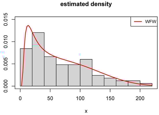
Figure 3. Fitted WFW density to COVID-19 mortality dataset.

8.3. COVID-19 Times Dataset

The dataset of reported COVID-19 cases, introduced by [35], comprises 30 recorded observations representing the spread of the disease over a specific time interval. These observations offer valuable insights into infection trends and patterns, facilitating a thorough analysis of the disease’s progression and predictive modeling. These observations are as follows: 14.918, 10.656, 12.274, 10.289, 10.832, 7.099, 5.928, 13.211, 7.968, 7.584, 5.555, 6.027, 4.097, 3.611, 4.960, 7.498, 6.940, 5.307, 5.048, 2.857, 2.254, 5.431, 4.462, 3.883, 3.461, 3.647, 1.974, 1.273, 1.416, and 4.235. For more details, see [35]. This dataset requires appropriate statistical modeling techniques to capture their underlying patterns effectively. Therefore, to evaluate the ability of various distribution models to describe the observed trends, different statistical models are fitted to the dataset (see Table 8). The fitting results are presented in the following sections. Based on the low values of AIC, BIC, and HQIC, the WFW model emerges as the best option for describing this dataset (see Table 9). The FW and EW models also demonstrate a good performance, while the KwW model provides the weakest fit. Therefore, the WFW model is recommended for analyzing the COVID-19 times dataset.

Table 8. Estimates of the fitted models for COVID-19 times data.

Model	Parameter 1	Parameter 2	Parameter 3	Parameter 4
WFW$(\theta ,\lambda )$	0.127 (0.015)	3.951 (0.931)
GFW$(a,\alpha ,\beta )$	0.3418 (0.566)	0.1315 (0.07)	16.38 (24.75)
FW$(\theta ,\lambda )$	0.1199 (0.018)	5.596 (1.056)
EW$(\alpha ,\lambda ,\beta )$	4.084 (3.476)	1.188 (0.679)	2.508 (3.049)
KwW$(a,b,\lambda ,k)$	100 (1472.02)	100 (960.966)	2.444 (13.220)	0.1249 (0.6912)
W$(\alpha ,\beta )$	6.9637 (0.715)	1.879 (0.262)
LNORM$(\mu ,\sigma )$	1.6471 (0.112)	0.611 (0.078)

Table 9. Adequacy measures for of the fitted models for COVID-19 times dataset.

Model	AIC	CAIC	BIC	HQIC
WFW$(\theta ,\lambda )$	157.7342	158.1787	159.5366	158.6308
GFW$(a,\alpha ,\beta )$	158.677	159.6	162.8806	160.0217
FW$(\alpha ,\beta )$	158.810	158.2553	160.6132	158.7073
KwW$(a,b,\lambda ,k)$	161.3179	162.9179	166.9226	163.1109
W$(\alpha ,\beta )$	158.0685	158.5129	160.8709	158.965
LNORM$(\mu ,\sigma )$	158.4702	159	161.2726	159.3667

9. ${\mathrm{MOP}}_{\left[\mathit{P}\right]}$ Assessments and Risk Analysis Under Real Data

The PORT-VaR estimator helps in identifying and analyzing extreme events or outliers in COVID-19 data. Peaks over a specified VaR threshold may represent unusual or critical situations, such as sudden spikes in infection rates, hospitalizations, or other medical metrics related to COVID-19 [13,36,37]. Below, three subsections are presented: the first focuses on ${\mathrm{MOP}}_{\left[P\right]}$ assessments and the optimal order of P based on the true mean value (TMV), the second examines the PORT-VaR estimator under failure time data, and the third explores the PORT-VaR estimator in the context of medical data.

9.1. ${\mathit{MOP}}_{\left[P\right]}$ Assessments and Optimal Order of P

Following [27], selecting the optimal order of P is crucial for ${\mathrm{MOP}}_{\left[P\right]}$ assessments, as it balances capturing sufficient detail in risk profiles with avoiding overfitting or excessive complexity. Empirical and statistical analyses are employed to determine the ideal P, ensuring accurate representation of the underlying risk distribution. This process enhances robust risk evaluation and decision-making. Statistical tools like ${\mathrm{MOP}}_{\left[P\right]}$ distributions enable quantitative risk assessment, hazard identification, and effective mitigation strategies, empowering stakeholders to allocate resources efficiently and build resilience against uncertainties. Table 10 provides the ${\mathrm{MOP}}_{\left[P\right]}$ assessment, including the TMV, MSE, and Bias under $P=1,2,\dots ,5$, $n=1000$ and some different parameter values. Based on the results presented in Table 10 (the first scenario) for ${\mathrm{MOP}}_{\left[P\right]}$ assessments under different orders ($P=1,2,3,4,5$) and with specific parameter values (${\theta }_0=10,{\lambda }_0=2.5$) and a dataset size of $n=1000$, it is seen that the TMVs for ${\mathrm{MOP}}_{\left[P\right]}$ across all orders ($P=1,2,3,4,5$) remain stable around 1.001314, confirming a consistent estimate of the dataset’s true mean. The identical MSE values (0.9983274) indicate that prediction errors remain constant across different P orders, reflecting moderate deviation from the TMV. Similarly, the consistent bias values (0.9991634) suggest a systematic underestimation of the TMV. The stability of TMV, MSE, and bias across varying P orders highlights the robustness of ${\mathrm{MOP}}_{\left[P\right]}$, ensuring reliable mean estimation and prediction accuracy despite changes in model parameters and dataset size. Based on the results presented in Table 10 for the second scenario, ${\mathrm{MOP}}_{\left[P\right]}$ assessments are conducted under different orders ($P=1,2,3,4,5$) with specific parameter values (${\theta }_0=2,{\lambda }_0=1.5$) and a dataset size of $n=1000$. The TMVs for ${\mathrm{MOP}}_{\left[P\right]}$ across all orders remain stable at approximately 0.9973669, confirming consistent mean estimation. Additionally, identical MSE values (0.9947407) indicate a uniform level of prediction error across different P orders. Similarly, the bias values (0.9973669) consistently show a slight underestimation of the TMV. The stability of TMV, MSE, and bias across varying P orders highlights the robustness of ${\mathrm{MOP}}_{\left[P\right]}$, ensuring reliable mean estimation with predictable error levels regardless of parameter settings and dataset size. Across all parameter combinations and orders of P, the TMV estimates derived from ${\mathrm{MOP}}_{\left[P\right]}$ assessments remain relatively stable and close to the expected value, indicating the robustness of the method in estimating central tendencies within the dataset, with means stability of the TMV. The MSE and bias values also exhibit consistency across different orders of P and parameter settings. This suggests that while there is a predictable level of MSE and bias in the ${\mathrm{MOP}}_{\left[P\right]}$ estimates, these metrics remain relatively invariant to changes in the order of P and specific parameter values, which means a consistent MSE and consistent bias. The consistent performance of ${\mathrm{MOP}}_{\left[P\right]}$ across varied conditions underscores its reliability as a statistical tool for risk analysis. Despite potential variations in dataset characteristics or model parameters, ${\mathrm{MOP}}_{\left[P\right]}$ consistently provides estimates that capture meaningful aspects of risk distributions.

Table 10. ${\mathrm{MOP}}_{\left[P\right]}$ assessment under $n=1000$ and $P=1,2,3,4,5$.

$\mathit{P}\to$	1	2	3	4	5
${\alpha }_0=10,{\beta }_0=2.5$
TMV	1.001314
MSE	0.9983274	0.9983274	0.9983274	0.9983274	0.9983274
Bias	0.9991634	0.9991634	0.9991634	0.9991634	0.9991634
${\theta }_0=2,{\lambda }_0=1.5$
TMV	0.9973669
MSE	0.9947407	0.9947407	0.9947407	0.9947407	0.9947407
Bias	0.9973669	0.9973669	0.9973669	0.9973669	0.9973669
${\theta }_0=0.5,{\lambda }_0=0.5$
TMV	0.9978629
MSE	0.9957304	0.9957304	0.9957304	0.9957303	0.9957296
Bias	0.9978629	0.9978629	0.9978629	0.9978629	0.9978625
${\theta }_0=100,{\lambda }_0=50$
TMV	0.9988142
MSE	0.9976297	0.9976297	0.9976297	0.9976297	0.9976297
Bias	0.9988142	0.9988142	0.9988142	0.9988142	0.9988142

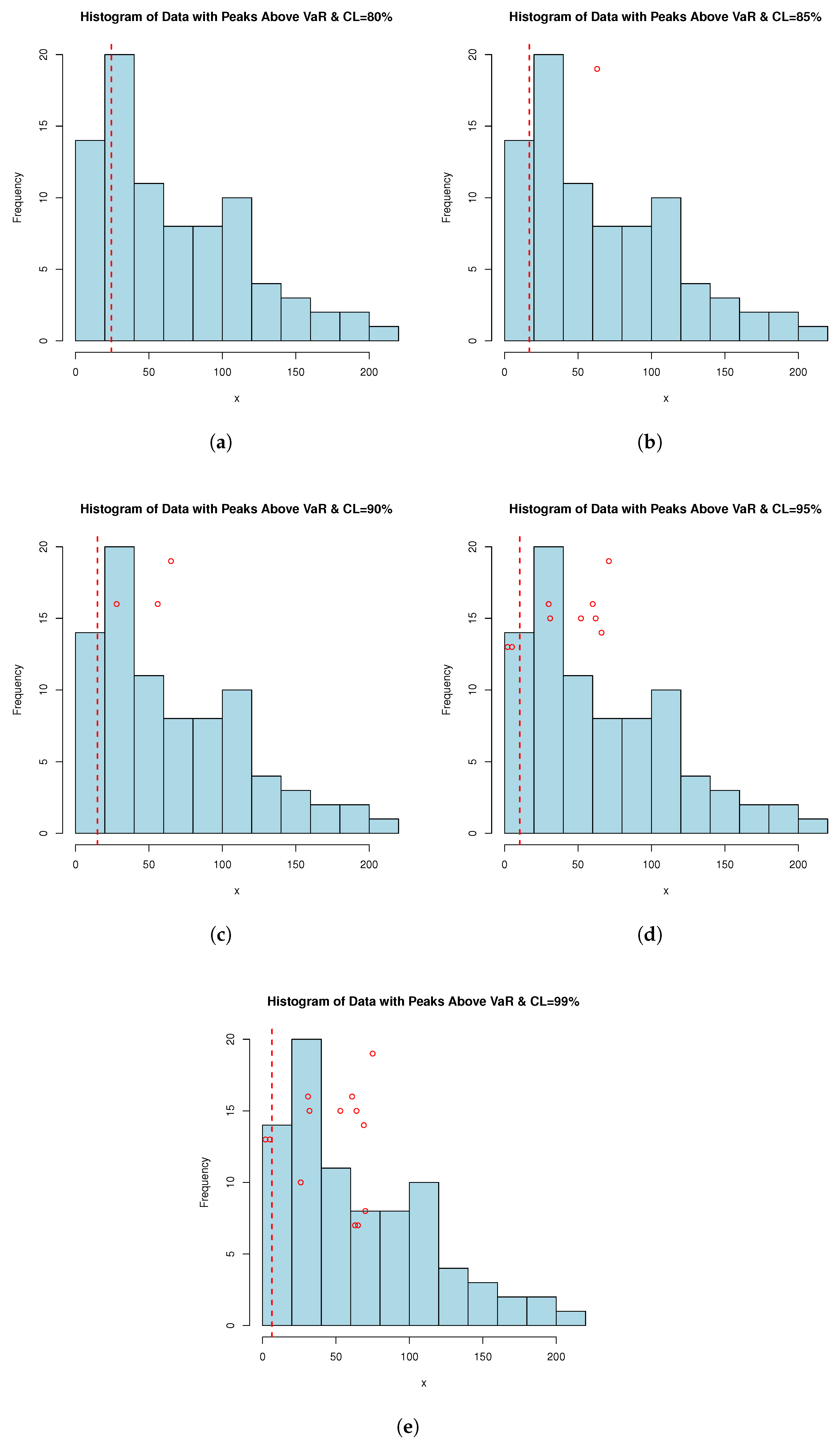
9.2. VaR, TVaR and PORT-VaR Estimators for Extreme Failure Times

Failure time datasets often represent the occurrence of critical events such as equipment failures, system breakdowns, or component malfunctions. By applying the PORT-VaR estimator, analysts can identify and quantify extreme failure events that exceed a specified risk threshold. This information is crucial for understanding the reliability profile of systems or components. PORT-VaR analysis allows for a deeper assessment of the risk and uncertainty associated with failure times. By setting a threshold based on the desired confidence level (e.g., 95% or 99%), researchers can evaluate the probability of experiencing extreme failures beyond this threshold. This insight helps in assessing the overall risk exposure and potential consequences of critical failures. In this subsection, the PORT-VaR analysis is presented under failure times data. A summary of the analysis results obtained at different confidence levels (CLs: 80%, 85%, 90%, 95%, and 99%) is presented in Table 11. The trend shows that, as CL increases, the inferences of PORT volume decreases. This trend characterizes a shift towards a safer risk assessment method, one that relies on a higher range to incorporate only the most extreme data present in the sample. This relationship is critical for risk tolerance measurement and risk management design when risk exposure is acceptable. Also, Figure 4 shows the PORT-VaR analysis for extreme failure times. Based on Table 11, as the CL increases, the number of identified PORTs generally decreases, reflecting stricter risk thresholds. Lower CLs (e.g., 80% and 85%) yield higher extreme event counts, indicating a greater prevalence of significant failure time events relative to the VaR threshold. The statistical distribution (Min, Median, Mean, Max) highlights variability in severity and frequency, offering key insights into the risk profile of failure times. These findings inform risk assessment and response strategies, helping identify areas requiring targeted interventions and resource allocation to mitigate elevated mortality risks. Understanding the distribution of extreme failure events across CLs aids in quantifying risk exposure, prioritizing mitigation efforts, and optimizing reliability and maintenance practices. Decision-makers can leverage these insights to allocate resources efficiently, implement targeted interventions, and enhance system resilience against extreme failures. Notably, as CL increases, the number of PORTs rises monotonically, while VaR and TVaR decrease, indicating that more extreme failure events are captured at higher CLs, though their severity declines over time. Managing risk based on VaR alone suggests that an 80–85% CL may be overly conservative, while 99% could underestimate extreme failure impacts. A balanced choice (e.g., 90–95%) might be optimal. However, at 99% CL, the number of exceedances doubles, meaning organizations must prepare for more frequent small-to-moderate failures rather than rare, catastrophic events.

Table 11. PORT-VaR analysis for extreme failure times.

CLs	N. of PORT	VaR	TVaR	Min.	1st Qu.	Median	Mean	3rd Qu.	Max.
80%	40	3.490	1.5764	0.148	0.586	3.067	4.158	6.410	15.08
85%	42	3.019	1.035	0.114	0.571	2.931	3.965	5.929	15.08
90%	45	1.491	0.593	0.086	0.381	2.054	3.708	4.893	15.08
95%	47	0.744	0.375	0.0740	0.3205	2.0060	3.5530	4.7135	15.08
99%	94	0.321	0.130	0.058	0.254	1.600	3.410	4.534	15.08

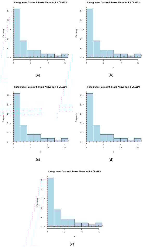
Figure 4. PORT-VaR analysis for extreme failure times. Each histogram is related to a confidence level (CL) of (a) 80%, (b) 85%, (c) 90%, (d) 95%, and (e) 99%.

9.3. VaR, TVaR, and PORT-VaR Estimators for Extreme COVID-19 Deaths

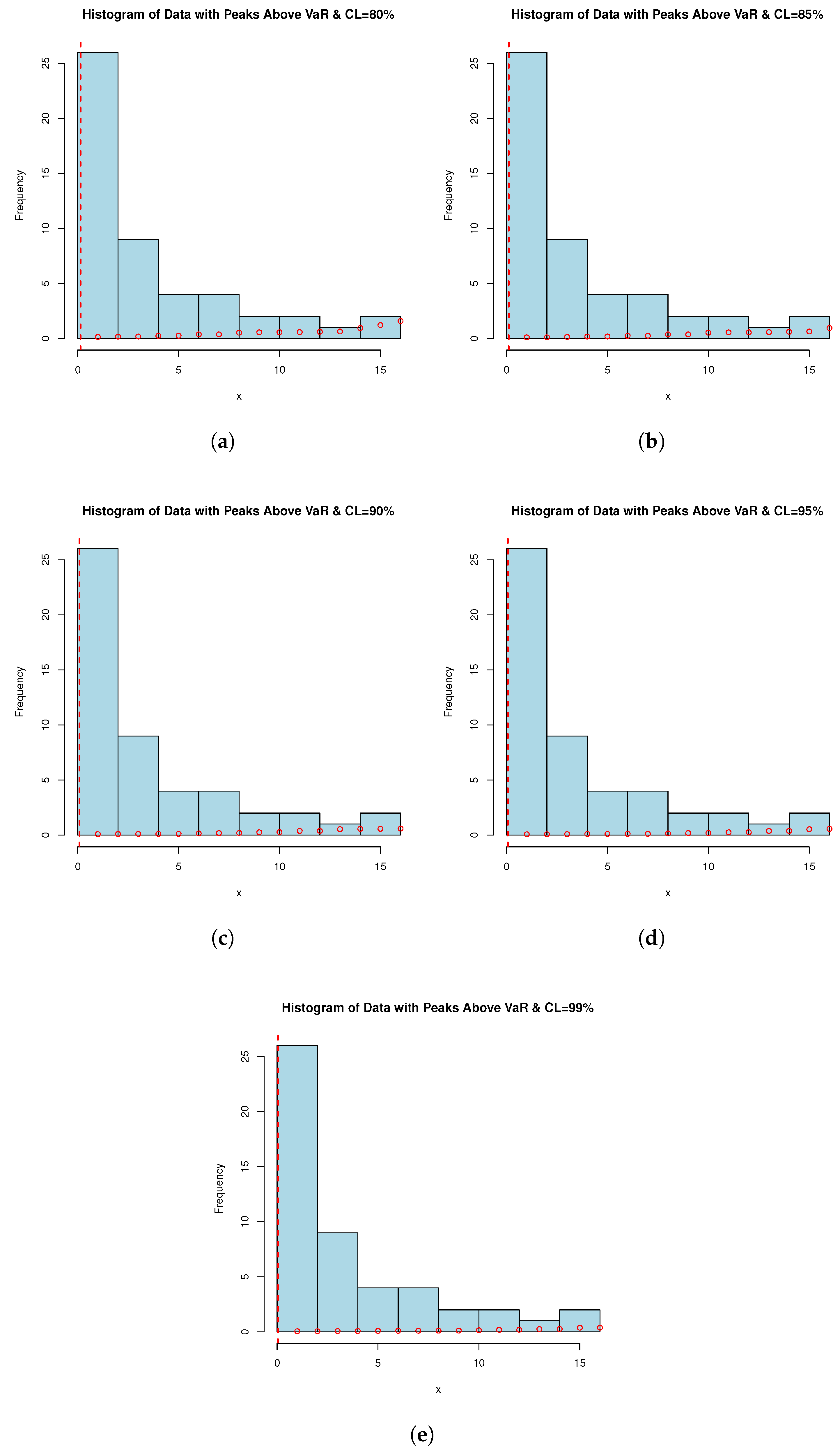
Analyzing PORT-VaR can aid in optimizing resource allocation within the medical sector. Identification of peaks over the VaR threshold allows for the focused allocation of healthcare resources, such as medical supplies, personnel, and hospital beds, to areas experiencing the highest levels of risk or demand during the pandemic. Insights from the PORT-VaR estimator can enhance decision-making processes and preparedness efforts. Healthcare facilities and public health authorities can use this information to develop robust contingency plans, allocate budgets effectively, and implement targeted interventions to address the emerging challenges highlighted by the peaks in COVID-19 data; for more applications, see [38,39]. According to [28], effective public health responses rely on timely and accurate data analysis. The PORT-VaR approach offers a quantitative framework to monitor and respond to evolving COVID-19 trends. It enables proactive measures to contain outbreaks, implement targeted vaccination campaigns, and mitigate the impact of unforeseen events. PORT-VaR analysis contributes to evidence-based research and policy development in the medical sector. Insights gained from studying peaks over the VaR threshold can inform the design of public health policies, clinical guidelines, and research priorities aimed at combating the COVID-19 pandemic. For this purpose, Table 12 is presented; it provides the PORT-VaR analysis under COVID-19 data. Table 12 provides valuable insights into the distribution and characteristics of extreme events (PORTs), identified using the VaR estimator under different confidence levels. These findings have practical implications for risk assessment, decision-making, and resource allocation in the context of COVID-19 dataset analysis and pandemic response efforts, where minimum (Min.) refers to the smallest PORT value observed above the VaR threshold and maximum (Max.) refers to the largest PORT value observed above the VaR threshold. However, the mean column refers to the average value of the PORT distribution, indicating the central tendency of extreme events. Finally, median refers to the middle value of the PORT distribution, separating the higher and lower halves of the data. Moreover, Figure 5 shows the PORT-VaR analysis for extreme COVID-19 deaths.

Table 12. PORT-VaR analysis for extreme COVID-19 deaths.

CL	N. of PORT	VaR	TVaR	Min.	1st Qu.	Median	Mean	3rd Qu.	Max.
80%	66	24.4	30.375	25.00	40.25	72.50	81.74	107.75	201.00
85%	70	16.9	11.769	19.00	38.00	70.50	78.29	107.00	201.00
90%	72	15	11	16.00	37.50	68.00	76.56	107.00	201.00
95%	78	10.3	7.2	13.00	32.50	58.50	71.76	103.25	201.00
99%	82	6.46	4	7.00	30.25	57.50	68.65	101.00	201.00

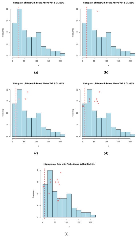
Figure 5. PORT-VaR analysis for extreme COVID-19 deaths. Each histogram is related to a confidence level (CL) of (a) 80%, (b) 85%, (c) 90%, (d) 95%, and (e) 99%.

Table 12 presents the PORT-VaR analysis for COVID-19 data, where the PORT column indicates the count of extreme events exceeding the VaR threshold at different CLs. As CL increases, fewer extreme events are detected, reflecting stricter risk thresholds, while lower CLs (e.g., 80% and 85%) capture more frequent extreme events. Descriptive statistics of PORT values (Min., Median, Mean, Max.) highlight the severity and frequency of extreme cases. The analysis underscores the sensitivity of risk assessment to CL variations, aiding in resource allocation and pandemic response planning. Notably, as CL rises, PORT counts increase while VaR and TVaR decrease, suggesting that higher thresholds capture more extreme cases but reduce individual severity estimates. A CL of 90–95% may offer a balanced approach for policymakers, avoiding overly conservative or lenient risk assessments.

10. Conclusions and Limitations

This study introduces the weighted flexible Weibull distribution, and its main properties, including cumulative and residual cumulative entropy, are explored. A simulation study confirms the consistency of the MLEs for parameter estimation. Applications to real-world data, including failure times and COVID-19 datasets, demonstrate the model’s good competitive performance against other lifetime distributions. Additionally, peaks over a random threshold value-at-risk (PORT-VaR) estimators are developed for risk analysis in engineering and medicine. These estimators mark a significant advancement in quantitative risk assessment, offering tailored solutions for diverse challenges. The findings highlight the importance of PORT-VaR analysis in various fields, including public health and engineering, contributing to improved risk management strategies.

Future research could integrate advanced statistical techniques and predictive modeling to enhance the accuracy and robustness of PORT-VaR assessments. Comparative studies across different datasets and contexts could further refine their applicability for risk mitigation and decision-making in complex systems. The PORT-VaR analysis provides valuable insights for interdisciplinary risk analysis, addressing contemporary challenges across multiple domains. This study introduces several novel aspects of actuarial risk assessment, expanding beyond a review of existing concepts. It pioneers the use of weighted distributions in actuarial risk modeling, addressing a critical research gap and offering a fresh perspective on risk evaluation. Actuarial risk metrics are applied beyond traditional financial contexts to medical data, particularly in assessing COVID-19 risk and managing datasets with extreme values, highlighting the adaptability of actuarial methods across diverse fields. Additionally, a new estimation technique and a sequential sampling plan based on truncated life testing are introduced, enhancing the precision and efficiency of risk assessment models. Furthermore, the discussion on PORT-VaR has been expanded, offering a more detailed analysis of its significance and applicability in modern risk assessment scenarios. These contributions advance actuarial risk modeling methodologies and reinforce their relevance across multiple disciplines, supporting more robust and informed decision-making in risk management. The PORT-VaR analysis for COVID-19 data highlights the impact of CLs on risk assessment, with higher CLs detecting fewer extreme events due to stricter thresholds, while lower CLs capture more frequent occurrences. Descriptive statistics of PORT values provide insights into the severity and distribution of extreme cases, emphasizing the importance of selecting appropriate CLs for effective risk evaluation. The observed trend of increasing PORT counts alongside decreasing VaR and TVaR at higher CLs suggests that broader thresholds identify more extreme cases while moderating individual severity estimates. A CL range emerges as a balanced choice for policymakers, ensuring a comprehensive yet practical approach to pandemic response and resource allocation.

While this study introduces significant advancements in actuarial risk modeling and PORT-VaR analysis, several limitations should be acknowledged. First, the proposed weighted flexible Weibull distribution, though competitive, has been evaluated on a limited number of datasets. This model can be applied to broader real-world applications, including different domains and larger datasets, requires further validation. Second, the PORT-VaR estimators were developed and tested within specific contexts, such as engineering and medical risk analysis, but their performance in other industries remains unexplored. Additionally, the study assumes that extreme events follow particular statistical patterns, which may not always hold true in highly dynamic or unpredictable environments. Another limitation is that the study primarily relies on historical data, which may not fully account for evolving risk factors, policy changes, or unexpected future developments. While simulation studies confirm the consistency of estimation methods, real-world uncertainties could introduce biases or deviations not captured in the models. Finally, the selection of confidence levels (CLs) in PORT-VaR analysis is based on statistical reasoning and practical considerations, but the optimal choice may vary depending on specific risk tolerance levels and decision-making frameworks. Future works should address these limitations by expanding the application of the proposed methods to diverse datasets, exploring adaptive modeling approaches for evolving risks and refining PORT-VaR techniques to enhance robustness across various domains.

References

- Chen, Y.S.; Lai, S.B.; Wen, C.T. The influence of green innovation performance on corporate advantage in Taiwan. J. Bus. Ethics 2006, 67, 331–339. [Google Scholar] [CrossRef]
- Cordeiro, G.M.; Ortega, E.M.; Nadarajah, S. The Kumaraswamy Weibull distribution with application to failure data. J. Frankl. Inst. 2010, 347, 1399–1429. [Google Scholar] [CrossRef]
- Famoye, F.; Lee, C.; Olumolade, O. The beta-Weibull distribution. J. Stat. Appl. 2005, 4, 121–136. [Google Scholar]
- Xie, M.; Tang, Y.; Goh, T.N. A modified Weibull extension with bathtub-shaped failure rate function. Reliab. Eng. Syst. Saf. 2002, 76, 279–285. [Google Scholar] [CrossRef]
- Xie, M.; Lai, C.D. Reliability analysis using an additive Weibull model with bathtub-shaped failure rate function. Reliab. Eng. Syst. Saf. 1996, 52, 87–93. [Google Scholar] [CrossRef]
- Mustafa, A.; El-Desouky, B.S.; AL-Garash, S. The Marshall-Olkin Flexible Weibull Extension Distribution. arXiv 2016, arXiv:1609.08997. [Google Scholar]
- Bebbington, M.; Lai, C.D.; Zitikis, R. A flexible Weibull extension. Reliab. Syst. Saf. 2007, 92, 719–726. [Google Scholar] [CrossRef]
- Mustafa, A.; El-Desouky, B.S.; Al-Garash, S. The exponentiated generalized flexible Weibull extension distribution. Fundam. J. Math. Math. Sci. 2016, 6, 75–98. [Google Scholar]
- Amasyali, K.; El-Gohary, N.M. A review of data-driven building energy consumption prediction studies. Renew. Sustain. Energy Rev. 2018, 81, 1192–1205. [Google Scholar] [CrossRef]
- Zekri, A.R.N.; Youssef, A.S.E.D.; El-Desouky, E.D.; Ahmed, O.S.; Lotfy, M.M.; Nassar, A.A.M.; Bahnassey, A.A. Serum microRNA panels as potential biomarkers for early detection of hepatocellular carcinoma on top of HCV infection. Tumor Biol. 2016, 37, 12273–12286. [Google Scholar] [CrossRef]
- Alizadeh, M.; Afshari, M.; Cordeiro, G.M.; Ramaki, Z.; Contreras-Reyes, J.E.; Dirnik, F.; Yousof, H.M. A Weighted Lindley Claims Model with Applications to Extreme Historical Insurance Claims. Stats 2025, 8, 8. [Google Scholar] [CrossRef]
- Kharazmi, O.; Contreras-Reyes, J.E.; Balakrishnan, N. Optimal information, Jensen-RIG function and α-Onicescu’s correlation coefficient in terms of information generating functions. Phys. A 2023, 609, 128362. [Google Scholar] [CrossRef]
- Kuschel, K.; Carrasco, R.; Idrovo-Aguirre, B.J.; Duran, C.; Contreras-Reyes, J.E. Preparing Cities for Future Pandemics: Unraveling the influence of urban and housing variables on COVID-19 incidence in Santiago de Chile. Healthcare 2023, 11, 2259. [Google Scholar] [CrossRef] [PubMed]
- Zwillinger, D. Table of Integrals, Series, and Products; Elsevier: Amsterdam, The Netherlands, 2014. [Google Scholar]
- Ferreira, A.A.; Cordeiro, G.M. The gamma flexible Weibull distribution: Properties and Applications. Span. J. Stat. 2023, 4, 55–71. [Google Scholar] [CrossRef]
- Gradshteyn, I.S.; Ryzhik, I.M. Table of Integrals, Series, and Products; Academic Press: Cambridge, MA, USA, 2007. [Google Scholar]
- Chaudhry, M.A.; Zubair, S.M. Generalized incomplete gamma functions with applications. J. Comput. Appl. Math. 1994, 55, 99–124. [Google Scholar] [CrossRef]
- Di Crescenzo, A.; Longobardi, M. On cumulative entropies. J. Stat. Inference 2009, 139, 4072–4087. [Google Scholar] [CrossRef]
- Kharazmi, O.; Contreras-Reyes, J.E. Fractional cumulative residual inaccuracy information measure and its extensions with application to chaotic maps. Int. J. Bifurc. Chaos 2024, 34, 2450006. [Google Scholar] [CrossRef]
- Kharazmi, O.; Yalcin, F.; Contreras-Reyes, J.E. Cumulative residual Fisher information based on finite and infinite mixture models. Fluct. Noise Lett. 2025. [Google Scholar] [CrossRef]
- Psarrakos, G.; Toomaj, A. On the generalized cumulative residual entropy with applications in actuarial science. J. Comput. Appl. Math. 2017, 309, 186–199. [Google Scholar] [CrossRef]
- Rényi, A. On measures of entropy and information. In Proceedings of the Fourth Berkeley Symposium on Mathematical Statistics and Probability, Volume 1: Contributions to the Theory of Statistics; University of California Press: Berkeley, CA, USA, 1961; Volume 4, pp. 547–562. [Google Scholar]
- Contreras-Reyes, J.E. Mutual information matrix based on Rényi entropy and application. Nonlinear Dyn. 2022, 110, 623–633. [Google Scholar] [CrossRef]
- Kuhn, M.; Wing, J.; Weston, S.; Williams, A.; Keefer, C.; Engelhardt, A.; Cooper, T.; Mayer, Z.; Kenkel, B.; Team, R.C. Package ‘caret’. R J. 2020, 223, 48. [Google Scholar]
- R Core Team. A Language and Environment for Statistical Computing; R Foundation for Statistical Computing: Vienna, Austria, 2024; Available online: http://www.R-project.org (accessed on 17 February 2025).
- Alizadeh, M.; Afshari, M.; Contreras-Reyes, J.E.; Mazarei, D.; Yousof, H.M. The Extended Gompertz Model: Applications, Mean of Order P Assessment and Statistical Threshold Risk Analysis Based on Extreme Stresses Data. IEEE Trans. Reliab. 2024. [Google Scholar] [CrossRef]
- Rice, J.A. Mathematical Statistics and Data Analysis; Thomson/Brooks/Cole: Belmont, CA, USA, 2007; Volume 371. [Google Scholar]
- Szubzda, F.; Chlebus, M. Comparison of Block Maxima and Peaks Over Threshold Value-at-Risk models for market risk in various economic conditions. Cent. Econ. J. 2019, 6, 70–85. [Google Scholar] [CrossRef]
- Mudholkar, G.S.; Srivastava, D.K. Exponentiated Weibull family for analyzing bathtub failure-rate data. IEEE Trans. Reliab. 1993, 42, 299–302. [Google Scholar] [CrossRef]
- Lai, C.D.; Xie, M.; Murthy, D.N.P. A modified Weibull distribution. IEEE Trans. Reliab. 2003, 52, 33–37. [Google Scholar] [CrossRef]
- Cordeiro, G.M.; Vasconcelos, J.C.S.; dos Santos, D.P.; Ortega, E.M.; Sermarini, R.A. Three mixed-effects regression models using an extended Weibull with applications on games in differential and integral calculus. Braz. J. Probability Stat. 2022, 36, 751–770. [Google Scholar] [CrossRef]
- Paranaíba, P.F.; Ortega, E.M.; Cordeiro, G.M.; Pascoa, M.A.D. The Kumaraswamy Burr XII distribution: Theory and practice. J. Stat. Comput. Simul. 2013, 83, 2117–2143. [Google Scholar] [CrossRef]
- Marinho, P.R.D.; Silva, R.B.; Bourguignon, M.; Cordeiro, G.M.; Nadarajah, S. AdequacyModel: An R package for probability distributions and general purpose optimization. PLoS ONE 2019, 14, e0221487. [Google Scholar] [CrossRef]
- Murthy, D.P.; Xie, M.; Jiang, R. Weibull Models; John Wiley & Sons: Hoboken, NJ, USA, 2004. [Google Scholar]
- Ahmad, Z.; Almaspoor, Z.; Khan, F.; El-Morshedy, M. On predictive modeling using a new flexible Weibull distribution and machine learning approach: Analyzing the COVID-19 data. Mathematics 2022, 10, 1792. [Google Scholar] [CrossRef]
- Brown, A.; Williams, R. Equity implications of ride-hail travel during COVID-19 in California. Transp. Res. Rec. 2023, 2677, 1–14. [Google Scholar] [CrossRef]
- Mohamed, H.S.; Cordeiro, G.M.; Minkah, R.; Yousof, H.M.; Ibrahim, M. A size-of-loss model for the negatively skewed insurance claims data: Applications, risk analysis using different methods and statistical forecasting. J. Appl. Stat. 2024, 51, 348–369. [Google Scholar] [CrossRef] [PubMed]
- Golinelli, D.; Boetto, E.; Carullo, G.; Nuzzolese, A.G.; Landini, M.P.; Fantini, M.P. Adoption of digital technologies in health care during the COVID-19 pandemic: Systematic review of early scientific literature. J. Medical Internet Res. 2020, 22, e22280. [Google Scholar] [CrossRef] [PubMed]
- Mohamed, E.B.; Souissi, M.N.; Baccar, A.; Bouri, A. CEO’s personal characteristics, ownership and investment cash flow sensitivity: Evidence from NYSE panel data firms. J. Econ. Financ. Adm. Sci. 2014, 19, 98–103. [Google Scholar] [CrossRef]
Disclaimer/Publisher’s Note: The statements, opinions and data contained in all publications are solely those of the individual author(s) and contributor(s) and not of MDPI and/or the editor(s). MDPI and/or the editor(s) disclaim responsibility for any injury to people or property resulting from any ideas, methods, instructions or products referred to in the content. |
© 2025 by the authors. Licensee MDPI, Basel, Switzerland. This article is an open access article distributed under the terms and conditions of the Creative Commons Attribution (CC BY) license (https://creativecommons.org/licenses/by/4.0/).