Abstract
In this work, a Thau observer is designed based on a nonlinear third-order mathematical model described by ODEs, which captures the dynamics among insulin levels, -cells, and glucose concentration. The novelty of this research lies in its interdisciplinary approach to understanding a complex biological system. The observer’s mathematical validation is established using the Localization of Compact Invariant Sets to determine the domain of attraction and global knowledge about the system’s dynamic bounds. These bounds are used to compute the Lipschitz constant and the elements of the free gain matrix that satisfy the constraints for designing a Thau observer, such as the stability matrix and asymptotic stability. This analysis provides insights into how insulin levels evolve over time at various glucose concentrations, an essential step toward hardware implementation due to the system’s chaotic behavior. It also establishes a mathematical background that could contribute to treatment planning in future Digital Twins studies. Numerical simulations demonstrate that the observer can accurately track the dynamic behavior of the Diabetes Mellitus model analyzed in this work through in silico methods.
Keywords:
diabetes mellitus model; nonlinear analysis; Thau observer; insulin observation; compact invariant sets MSC:
93C10; 93C15; 93D05
1. Introduction
Diabetes Mellitus (DM) is one of the most common metabolic disorders, and it is estimated that by the year 2045, the situation may be more alarming than previously envisaged [1]. Recently, it has been reported that diabetes prediction can be achieved by using supervised machine learning [2], leading to prediabetes surveillance [3], which, according to the authors, represents a growing global burden.
The main reason why diabetes is dangerous over a prolonged period is the lack of insulin produced by the pancreas in the presence of a high glucose concentration. This condition can be inherited or caused by any factor related to health conditions of the pancreas [4]. Insulin is a hormone secreted by -cells located in response to glucose concentrations. The primary function of insulin is to distribute glucose to all the cells in the body via the bloodstream, where it is used as an energy source. Projections from the years 2010 to 2030 estimate that 154 million people with diabetes will be located in India and China alone [5], considering only population growth rates. Failing to take preventive measures for diabetes can lead to severe and irreversible health damage. This is why technological advances have introduced new techniques for administering insulin treatment, and one approach to studying DM is mathematical biology [6]. Developing and personalizing a mathematical model that accurately represents an entire or partial population is challenging when considering only factors such as insulin, glucose, -cells, and insulin treatments, including rapid-acting, short-acting, intermediate-acting, and long-acting insulins. Nevertheless, these models further explain how each factor interacts with the immune system [7]. This paper focuses on the mathematical analysis of nonlinear dynamics described by ODEs [8], in which the design of a nonlinear observer is achieved by computing a Lipschitz constant based on the compact invariant set method for localization in open-loop scheme analysis. The purpose of our research is to continuously observe and monitor a patient’s health state while minimizing additional costs and avoiding unnecessary invasiveness [9].
One approach to studying Type 1 Diabetes Mellitus (DM1) involves numerical methods and statistical techniques, which are commonly used to solve these models [10]. However, this approach is not entirely feasible for understanding biological processes due to their chaotic behavior [11]. In 2011, Little et al. [12] established that every diabetes model exhibits nonlinear properties and chaotic dynamics, even when designing a closed-loop glucose controller using a linear model derived from clinical data. Although the literature extensively covers the insulin–glucose relationship, previous research has overlooked the implementation of a nonlinear ODE-based biological model with chaotic behavior. In 2013 [13], the first comparison between the Van der Pol oscillator and the dynamics of DM1 was made, proving that the biological model is nonlinear and highly sensitive to initial conditions. This background allows us to discern a strategy for studying and analyzing DM1 by implementing nonlinear control techniques to address its chaotic behavior. Furthermore, a recent study [14] reported that the application of closed-loop blood glucose regulation in patients with Type 1 diabetes could be achieved through an artificial pancreas, thus improving the effectiveness of postprandial blood glucose control by extending the Bergman physiological model with a digestion kinetics equation. The ODE model of interest was introduced in [15] and has been mathematically studied using an adaptive controller [16] and a backstepping sliding mode controller [17]. The concept of Digital Twins [18] has a significant impact on innovation in the context of DM1. However, designing a nonlinear observer using the Lipschitz constant involves a mathematical estimation technique that is used to infer unmeasured states of a system based on a nonlinear model and limited observable data. Compared to Digital Twins, an observer is primarily used in real-time systems, such as artificial pancreas technologies, to enhance the precision of insulin delivery by estimating unmeasured physiological states. Digital Twins are broader, predictive, and simulation-focused, while nonlinear Thau observers are narrower, real-time estimation tools. Applying a Thau observer to a nonlinear model of DM1 provides a solid mathematical foundation to support treatment planning and serves as the groundwork for future Digital Twins research. As a result, our work makes a meaningful contribution to the field of biomathematics.
This paper presents a mathematical analysis of the complex interactions among insulin, glucose, and -cells in the dynamic evolution of DM1. Using the LCIS, the minimum and maximum concentrations of each state variable in the system are determined, along with their evolution over time, demonstrating the boundedness of the system even in the presence of chaos. Additionally, conditions are established to support the design of the Thau observer. Using the maximum concentrations, the Lipschitz constant is computed to satisfy Thau’s inequality, ensuring that the observer is asymptotically stable. Finally, a Thau observer is designed to accurately estimate insulin concentrations, even in the presence of unforeseen disturbances. This observer is particularly helpful for biological systems where measurements are often affected by noise, sensor limitations, and external perturbations. The proposed methodology ensures that the estimated insulin values remain stable and reliable under different physiological conditions. To validate the performance and robustness of the proposed observer, a series of in silico experiments are conducted, simulating various dynamic scenarios, including both normal and pathological conditions. These experiments demonstrate the observer’s ability to track insulin levels with high precision and resilience against external perturbations. The results confirm that the Thau observer can be an effective tool for monitoring and analyzing insulin–glucose dynamics, contributing to the development of advanced control strategies for diabetes management.
The remainder of this paper is organized as follows. Section 2 presents the mathematical details of the model and how it describes the dynamical behavior of Diabetes Mellitus. Section 3 introduces the mathematical preliminaries of the Localization of the Compact Invariant Set method and its application to the model under study. Section 4 discusses Thau’s observer preliminaries, its design, and the computation of the Lipschitz constant. Simulations and experimental results are presented in Section 5. Finally, Section 6 and Section 7 present the discussion and conclusions of this work.
2. ODE Model
ODE models of diabetes typically aim to simulate the interactions among insulin secretion, glucose metabolism, and other physiological variables, such as insulin sensitivity and insulin resistance [19]. These models can range from simple representations of glucose–insulin dynamics to more complex systems incorporating multiple feedback loops, such as the effect of -cells function, meal intake, and physical activity [20]. By incorporating both physiological principles and empirical data, ODE models offer valuable insights into the mechanisms of diabetes, help predict patient-specific outcomes, and support the development of therapeutic strategies.
The model under study describes the interaction of three population densities: insulin, glucose, and -cells [15]. The significance of this model lies in the inclusion of -cells as a regulatory agent, whereas the relationship between insulin and glucose exhibits characteristics similar to the predator–prey dynamics in the Lotka–Volterra model, where insulin acts as the predator and glucose as the prey. However, the presence of -cells does not alter the chaotic behavior associated with the Lotka–Volterra model [21], even when -cells are included. Therefore, the model is formulated using a set of nonlinear ordinary differential equations, as follows:
where is the population density of the predator (insulin), is the population density of the prey (glucose), and is the population density of the -cells. The parameters and only have numerical values. If and are zero, the attractor remains. The numerical values of the system’s parameters are presented below in Table 1.

Table 1.
Dimensionless parameters proposed in [15].
3. Materials and Methods
3.1. Mathematical Preliminaries
This section addresses general theorems used to determine the bounds of a system. Starkov and Krishchenko outlined a general localization method for nonlinear systems in their works [22,23]. The proposed methodology focuses on identifying and analyzing compact invariant sets in nonlinear dynamical systems. These sets facilitate a localized examination of the system’s behavior, reducing complexity while preserving essential dynamics. Recent research has shown that the compact invariant set localization method (LCIS) is valid and provides a deeper understanding of the nonlinear ODE model [24].
To understand the LCIS method, the methodology can be synthesized into the following key steps:
- Define the nonlinear system. Represent the system with a set of ODEs in the following form:where is a -differental vector field.
- Let be a differentiable function such that h is not the first integral of the system (2); therefore, the function is used as a solution to the problem of localization of all compact invariant sets and is called the localizing function. Let be the restriction of h to a set
- If the localization is set and all compact invariant sets are considered inside the domain , then the localization set is valid, with defined in Theorem 1. Let Q be a subset of . Then, the following theorem applies:
Theorem 1.
Each compact invariant set Γ of (2) is contained in the localization set [22].
- 4.
- A refinement of the localization set is achieved with the help of the iterative theorem, which is stated as follows:
Proposition 1.
If then the system (2) has no compact invariant sets located in Q [22].
- 5.
- The mathematical expression corresponds to the theorem defined in [25], known as the iterative theorem, which is described as follows:
Theorem 2.
Let be a sequence of function of [23], then
and
then, it contains any compact invariant set of the system (2) and
- The advantage of this methodology lies in the fact that it can generate upper or lower bounds by combining several localizing functions. There is no limit to the number of localizing functions that can be combined to obtain a higher upper bound or a smaller lower bound. These criteria depend on the specific research; the key aspect of the method is to obtain one upper or lower bound for each state variable that is part of the nonlinear system.
- 6.
- This section reviews valuable results from these works. First, it is assumed that all state variables are positive and located in the positive orthant, , giving biological meaning. Also, consider as the closed set :The solution to the problem of localizing the compact invariant sets is limited to the positive invariant compact sets; therefore, the goal is to find the maximum densities of each variable to define the region.
3.2. Analyzing the Nonlinear ODE Model of DM1
Since and are free constant parameters that represent the instantaneous dose of insulin and glucose concentration, respectively, each depends on a specific moment of the day. If we assume the condition , this represents a steady state where no food is consumed, and, therefore, insulin inactivation is maintained. On the other hand, if , , this implies that insulin is activated due to glucose consumption at a given initial condition. In both cases, the system’s set of equations in (1) has an attractor and retains its nonlinear properties. Therefore, nonlinear theory provides a broader understanding of the complex behavior of these types of systems. In this context, the localization method is applied. The system (1) is considered under the condition , , which ensures that the system operates within a positive domain. Comparing with Equation (2), the following localizing function is defined:
where q is a free positive parameter. Hence, considering , the expression defined by , and after applying the Lie derivative to the function (3), the set is defined as the set containing the Lie derivative, i.e., , which is represented by:
now, substituting Equation (4) into Equation (3) results in the set , which is defined as:
by grouping common terms with respect to and performing algebraic manipulation, can be expressed as:
Therefore, the compact invariant set is defined as follows:
giving as a result the maximum concentration of insulin and the minimum concentration of glucose, which are defined as follows:
Now, to establish an upper bound for the population density of glucose, consider a second localization function, , defined as follows:
after applying the Lie derivative to , setting , and performing some algebraic rearrangement, is given by:
this leads to the upper bound for the set , given by:
this allows the maximum concentration of glucose to be defined by the set , as follows:
Therefore, the lower and upper bounds for the glucose concentration are mathematically defined by the set:
Finally, the last localization function, in order to define an upper bound for the cells, is:
after applying the previous steps to the proposed localization function (11), we obtain the set , given by:
This allows the maximum concentration of -cells to be defined as follows:
As a result of the previous analysis, the following theorem can be stated:
Theorem 3.
Defining a non-empty set in diabetes models is a compelling topic due to the mathematical complexity involved in representing nonlinear systems. However, on the basis of in silico experimentation, the results obtained are well-defined. Our findings contribute to demonstrating that the behavior of DM1 is inherently nonlinear, warranting further investigation from a mathematical perspective.
The work presented in [26] is particularly notable for introducing and evaluating the use of computational models in clinical trial design, an emerging methodology at the time. The authors propose a mathematical model that simulates the systemic inflammatory response in patients, allowing the prediction of therapeutic intervention outcomes without the need for traditional clinical trials. This approach has the potential to optimize clinical study designs, reduce costs, and improve patient safety by anticipating potential adverse effects.
In alignment with these advancements, we propose a threshold value for q such that .
4. Nonlinear Observer
The challenge of designing observers specifically tailored for nonlinear control systems was first introduced by Thau in his seminal work [27]. Over the past four decades, the control systems literature has evolved significantly, leading to the development of various methodologies for constructing observers that operate effectively in nonlinear frameworks [28]. These nonlinear observers have been applied across diverse fields, addressing key challenges, such as state estimation, parameter estimation, fault detection and isolation, disturbance estimation, and unknown input estimation. In 1998, a significant nonlinear observer was introduced to evaluate the validity of a biological model focused on phytoplanktonic growth [29]. However, subsequent research by Gabriele underscored the importance of parameter estimation in systems biology, highlighting its crucial role in generating meaningful predictions from computational models designed to represent biological systems accurately [30]. These insights have profound implications for computational biology, providing powerful tools to analyze and understand complex biological phenomena.
The use of state observers has also been explored in other biological processes, demonstrating their effectiveness in estimating variables that are difficult to measure directly. For instance, in [31], a robust observer was implemented to monitor ethanol fermentation in real time, enabling accurate inferences about key process variables. This approach is analogous to insulin and glucose estimation in this work, where the observer is used to infer non-measurable states in the glycemic regulation system.
Furthermore, mathematical modeling of glucose supply has been addressed in [32], where incomplete functions were used to describe system dynamics. This approach provides a relevant mathematical framework for formulating the model in this work, enhancing the accuracy of insulin and glucose estimation through the integration of observer techniques. These contributions underscore the growing role of control theory in computational biology, reinforcing the importance of state observers in developing reliable models for physiological processes.
In recent years, computational biology has turned to control theory to tackle the issue of parameter estimation, particularly through the use of state observers. Initially formulated for state estimation tasks, these algorithms aim to deduce the time evolution of unobserved components within a dynamical system. The existing literature on control theory in this context is extensive, with several classical techniques, such as Luenberger-like observers [33], being employed in biological or biochemical systems. A key advancement in nonlinear observer design for population biology models came with the application of Sundarapandian’s theorem to the Lotka–Volterra model, which describes two-species competition with stable coexistence [34].
Despite the variety of available observer designs, Thau’s observer has emerged as a particularly robust method. Its strength lies in its reliability in providing sufficient information about a system’s trajectory over time, primarily due to its incorporation of a Lipschitz constant. This constant plays a crucial role in characterizing system behavior within chaotic regimes. In this context, it is possible to define a domain that encompasses the system’s trajectories, often represented as an ellipsoid, thus facilitating the determination of the Lipschitz constant. This approach not only enhances the understanding of trajectory behavior but also strengthens the robustness of observer design in managing the complexities inherent in nonlinear dynamics.
Thau Observer
Based on the set of equations from system (1), the following conditions must be satisfied for the observer design. First, the pair (C, A) must be observable. Second, the nonlinear function must be continuously differentiable and locally Lipschitz. If these two conditions are met, a nonlinear Thau observer can be constructed as:
Then, there exists a matrix that is symmetric and stable, with eigenvalues in the negative plane. In addition, there exists a positive matrix Q that is defined from a matrix P, which is determined by the Lyapunov equation as:
hance, if k is chosen such that satisfies Equation (16), let be the Lipschitz constant expressed in the following inequality:
where the Lipschitz constant must satisfy the following inequality:
for all and the error of the Thau observer will be globally asymptotically stable. By applying the theorem in [35], the observer can be obtained by satisfying the inequality:
Since the matrix is defined by the linear values of the equations in (1), and considering the state variables of the glucose and cells as potential variables needed to track the dynamical behavior of the observer over time, and to satisfy the symmetric restriction of , the parameters of the matrix k are chosen as ; with and for a stable . Hence, the extended form of is given by:
Meanwhile, the nonlinear terms of system (1) are expressed as follows:
Now, to satisfy inequality (17), the Frobenius norm is computed over the ellipsoidal domain where , and . The numerical solution for the Frobenius norm gives:
meanwhile, solving the inequality (17) numerically yields:
Therefore, based on Equation (15), the Thau observer for the system (1) is defined as follows:
5. Numerical Simulation and Results
The Thau observer estimates the system’s state variables based on the model’s equations and the measured output. When simulated alongside the actual system, it allows us to validate that the observer accurately tracks the states and assesses the convergence of the estimated states to the actual states over time, as shown in Figure 1, considering the parameters in Table 1. Figure 1 also presents the phase plane comparison for each state variable.
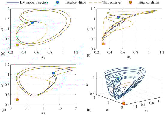
Figure 1.
Comparison between the system (1) and Thau observer estimation in the absence of perturbations, with and . This comparison ensures the Thau observer is correctly implemented and performs as expected under given conditions. In (a), the phase planes vs. and vs. are depicted. In (b), the phase planes vs. and vs. are shown. In (c), the phase planes vs. and vs. are illustrated. Finally, in (d), the chaotic behavior is demonstrated.
Perturbations in the system, such as carbohydrate intake, have been extensively studied in the literature [36]. These perturbations are incorporated to simulate realistic scenarios in diabetic patients, where external factors significantly affect the dynamics of glucose and insulin. In this study, a nonlinear observer is used to estimate the system’s states under these conditions by adjusting the population density by a finite factor at specific time intervals. The observer’s estimation accuracy is demonstrated in Figure 2, which compares the system’s actual states with those estimated by the Thau observer. The perturbations introduced in the initial stage are shown in Figure 3, which illustrates how the observer minimizes the estimation error and confirms its stability and robustness under various initial conditions or disturbances. Additionally, Figure 4 displays the error dynamics for each state variable, showing that all errors asymptotically converge to zero within a few seconds, even in the presence of perturbations.
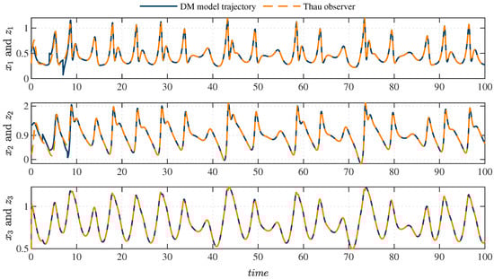
Figure 2.
Comparison between the system (1) and the Thau observer. Solid lines indicate actual state trajectories, while dashed lines indicate estimated state trajectories from the observer. Perturbations are introduced prior to ; nevertheless, the observer’s trajectories consistently track the system’s patterns.
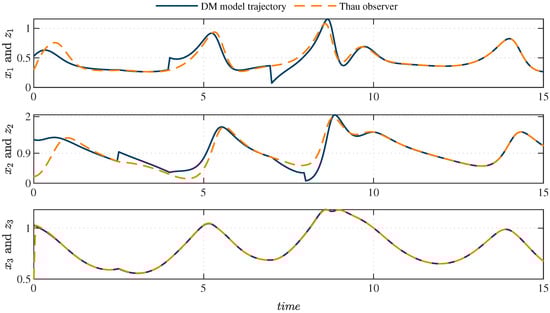
Figure 3.
Comparison between the system (1) and the Thau observer. Perturbations are applied to the insulin population density, with values of and at and , respectively. Similarly, perturbations of and are applied to the glucose population density at and , respectively.
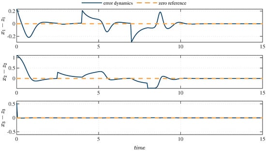
Figure 4.
Error dynamics. Accurate estimation enhances control efficiency, robustness to disturbances, and overall system reliability, making error minimization essential for effective observer performance. As presented in this figure, at 10.5 s, the estimated error can be considered almost zero for , and follows the dynamics of (1). Similarly, at 0.6 s, the state also aligns with the system’s dynamics.
The simulations were performed using the ode45 function in MATLAB® R2023b (The MathWorks, Inc., Natick, MA, USA), with a maximum step size of [37]. This solver, which utilizes a fourth- and fifth-order Runge–Kutta algorithm, was employed to validate the derived conditions mathematically. In this research, direct comparisons with real-world measurements are not initially conducted, as the primary focus is to analyze the biological dynamic behavior of this type of model over time through mathematical modeling. Future work will compare these results with real-world conditions documented in the literature.
6. Discussion
Designing a Thau observer for model (1) focuses on nonlinear DM1 systems, enabling the management of complex nonlinear behaviors and leading to more accurate trajectory tracking in nonlinear models [38], as shown in Figure 1 and Figure 2. The dimensionless parameters in Table 1 exhibit chaotic behavior if and only if parameters and are less than or equal to . Other values of those parameters must be studied and analyzed for deeper biological implications. For example, in [39], computational and mathematical modeling approaches for drug development are discussed as advantageous due to their fast predictive capability and cost-effectiveness features. In future research, we will exploit the feasibility of implementing a comparative analysis considering our results with the Digital Twins predictions [40] to explore deeper biological implications. In addition, we will study the design of a nonlinear controller based on the designed observer, contributing to the approach of the implementation of new technology [41]. The LCIS method remains a key mathematical strategy for analyzing nonlinear ODE models with biological implications [24]. Therefore, the importance of nonlinear control theory applied in biomathematics can significantly enhance results. The Thau observer for the nonlinear DM model that considers -cell dynamics allows accurate estimation of insulin levels, even under impaired -cell functionality. It integrates the nonlinear interactions between glucose and insulin while reducing reliance on invasive measurements. The observer provides real-time insights into -cell contributions, improving personalized diabetes management and treatment strategies. For instance, in Figure 3, the observer effectively manages uncertainties and disturbances in the system, ensuring reliable insulin level predictions. In Figure 4, the performance of the Thau observer is critical for ensuring accurate state estimation, system stability, and precise trajectory tracking. Significant errors can lead to unreliable state feedback, degraded control performance, and deviations from desired behavior.
7. Conclusions
This paper presents a Thau observer for a Diabetes Mellitus model that describes the dynamic interaction among insulin, glucose, and -cells. The observer can estimate insulin levels by measuring the glucose and population of -cells. However, designing a Thau observer is not easy; this type of observer requires certain conditions that must be satisfied, such as the Lipschitz constant and the stability matrix . Therefore, there are established conditions for the free feedback matrix k such that all eigenvalues of the stability matrix defined by have a negative real part. Next, LCIS analysis is applied to determine the sets containing the dynamical behaviors of each state variable, defined by (14) considering the dimensionless parameters described in Table 1, to guarantee the stability condition established by inequality (17), needed to ensure the observer’s asymptotic stability. Furthermore, the observer’s performance and asymptotic stability are verified through MATLAB® simulations. Future work will focus on closed-loop control analysis and mathematical validation of the entire system, along with its implementation on a digital platform to develop a Digital Twin system. Both the conceptual Digital Twin and the closed-loop control system will enable the exploration of complex scenarios that would be dangerous or infeasible in real-life experiments due to validated treatment protocols. In addition, this approach will allow the study of perturbed cases influenced by factors such as caloric intake, exercise routines, and sleep patterns, facilitating the design of personalized treatment protocols. By integrating patient-specific data and real-time monitoring, the Digital Twin system has the potential to serve as an advanced simulation tool for predicting glucose–insulin dynamics under various physiological and pathological conditions. This will provide clinicians with a deeper understanding of the metabolic response of individuals, allowing for more precise treatment adjustments. Beyond individual treatment optimization, the implementation of a Digital Twin system could contribute to broader diabetes research by simulating large-scale population dynamics and testing novel therapeutic strategies before clinical trials. This would reduce the risks and costs associated with experimental treatments while improving the reliability of medical interventions. Ultimately, this research aims to improve the management of diabetes by offering a robust and patient-specific approach that minimizes the risks associated with hyperglycemia and hypoglycemia.
Author Contributions
Formal analysis and investigation, D.G.; software and validation, T.C.G.; writing—review and editing, P.J.C. All authors have read and agreed to the published version of the manuscript.
Funding
This research received funding from the Tecnológico Nacional de México/Instituto Tecnológico de Tijuana through the titled projects: ESTUDIO DE LA DIABETES MELLITUS TIPO 1 COMO UNA ENFERMEDAD MULTIFACTORIAL with ID 20136.24-P, and SISTEMA AUTÓNOMO DE REGULACIÓN DE INSULINA Y EXPERIMENTACIÓN IN-SILICO PARA TRATAMIENTOS DE LA DIABETES MELLITUS TIPO 1 with ID 23154.25-P.
Data Availability Statement
The detailed data supporting the findings of this article are available from the authors upon request. All original contributions presented in this study are included in the article. For further inquiries, please contact the corresponding authors.
Conflicts of Interest
The authors declare no conflicts of interest.
References
- Saeedi, P.; Petersohn, I.; Salpea, P.; Malanda, B.; Karuranga, S.; Unwin, N.; Colagiuri, S.; Guariguata, L.; Motala, A.A.; Ogurtsova, K.; et al. Global and regional diabetes prevalence estimates for 2019 and projections for 2030 and 2045: Results from the International Diabetes Federation Diabetes Atlas, 9th edition. Diabetes Res. Clin. Pract. 2019, 157, 107843. [Google Scholar] [CrossRef] [PubMed]
- Febrian, M.E.; Ferdinan, F.X.; Sendani, G.P.; Suryanigrum, K.M.; Yunanda, R. Diabetes prediction using supervised machine learning. Procedia Comput. Sci. 2023, 216, 21–30. [Google Scholar] [CrossRef]
- Rooney, M.R.; Fang, M.; Ogurtsova, K.; Ozkan, B.; Echouffo-Tcheugui, J.B.; Boyko, E.J.; Magliano, D.J.; Selvin, E. Global prevalence of prediabetes. Diabetes Care 2023, 46, 1388–1394. [Google Scholar] [CrossRef] [PubMed]
- Antar, S.A.; Ashour, N.A.; Sharaky, M.; Khattab, M.; Ashour, N.A.; Zaid, R.T.; Roh, E.J.; Elkamhawy, A.; Al-Karmalawy, A.A. Diabetes mellitus: Classification, mediators, and complications; A gate to identify potential targets for the development of new effective treatments. Biomed. Pharmacother. 2023, 168, 115734. [Google Scholar] [CrossRef]
- Shaw, J.; Sicree, R.; Zimmet, P. Global estimates of the prevalence of diabetes for 2010 and 2030. Diabetes Res. Clin. Pract. 2010, 87, 4–14. [Google Scholar] [CrossRef]
- Vallis, M.; Ryan, H.; Berard, L.; Cosson, E.; Kristensen, F.B.; Levrat-Guillen, F.; Naiditch, N.; Rabasa-Lhoret, R.; Polonsky, W. How continuous glucose monitoring can motivate self-management: Can motivation follow behaviour? Can. J. Diabetes 2023, 47, 435–444. [Google Scholar] [CrossRef] [PubMed]
- Shi, M.; Zhou, J.; Cai, M. Multiple Physiological and Behavioural Parameters Identification for Dietary Monitoring Using Wearable Sensors: A Study Protocol. medRxiv 2024. [Google Scholar] [CrossRef]
- Lakshmanan, M. Nonlinear dynamics: Challenges and perspectives. Pramana 2005, 64, 617–632. [Google Scholar] [CrossRef]
- Aliffi, G.E.; Nastasi, G.; Romano, V.; Pitocco, D.; Rizzi, A.; Moore, E.J.; De Gaetano, A. A system of ODEs for representing trends of CGM signals. J. Math. Ind. 2024, 14, 23. [Google Scholar] [CrossRef]
- Savatorova, V. Exploring parameter sensitivity analysis in mathematical modeling with ordinary differential equations. CODEE J. 2023, 16, 4. [Google Scholar] [CrossRef]
- Bortz, D.M.; Messenger, D.A.; Dukic, V. Direct estimation of parameters in ODE models using WENDy: Weak-form estimation of nonlinear dynamics. Bull. Math. Biol. 2023, 85, 110. [Google Scholar] [CrossRef]
- Little, R.R.; Rohlfing, C.L.; Sacks, D.B. Status of hemoglobin A1c measurement and goals for improvement: From chaos to order for improving diabetes care. Clin. Chem. 2011, 57, 205–214. [Google Scholar] [CrossRef]
- Wu, J.; Li, C.; Chen, W.; Lin, C.; Chen, T. Application of Van der Pol oscillator screening for peripheral arterial disease in patients with diabetes mellitus. J. Biomed. Sci. Eng. 2013, 6, 1143. [Google Scholar] [CrossRef]
- Liu, S.; Song, R.; Lu, X. Research on Blood Glucose Nonlinear Controller Based on Backstepping Adaptive Control Algorithm. In Proceedings of the 2024 IEEE 13th Data Driven Control and Learning Systems Conference (DDCLS), Kaifeng, China, 17–19 May 2024; pp. 472–477. [Google Scholar] [CrossRef]
- Shabestari, P.S.; Panahi, S.; Hatef, B.; Jafari, S.; Sprott, J.C. A new chaotic model for glucose-insulin regulatory system. Chaos Solitons Fractals 2018, 112, 44–51. [Google Scholar] [CrossRef]
- Singh, P.P.; Singh, K.M.; Roy, B.K. Chaos control in biological system using recursive backstepping sliding mode control. Eur. Phys. J. Spec. Top. 2018, 227, 731–746. [Google Scholar] [CrossRef]
- Saoussane, M.; Mohammed, T.; Mesaoud, C. Adaptive controller based an extended model of glucose-insulin-glucagon system for type 1 diabetes. Int. J. Model. Simul. 2023, 43, 282–293. [Google Scholar] [CrossRef]
- Mosquera-Lopez, C.; Jacobs, P.G. Digital twins and artificial intelligence in metabolic disease research. Trends Endocrinol. Metab. 2024, 35, 549–557. [Google Scholar] [CrossRef]
- Ackerman, E.; Rosevear, J.W.; McGuckin, W.F. A mathematical model of the glucose-tolerance test. Phys. Med. Biol. 1964, 9, 203. [Google Scholar] [CrossRef]
- Dalla Man, C.; Breton, M.D.; Cobelli, C. Physical activity into the meal glucose—Insulin model of type 1 diabetes: In silico studies. J. Diabetes Sci. Technol. 2009, 3, 56–67. [Google Scholar] [CrossRef]
- Vano, J.; Wildenberg, J.; Anderson, M.; Noel, J.; Sprott, J. Chaos in low-dimensional Lotka Volterra models of competition. Nonlinearity 2006, 19, 2391–2404. [Google Scholar] [CrossRef]
- Krishchenko, A.P. Estimations of domains with cycles. Comput. Math. Appl. 1997, 34, 2–4. [Google Scholar] [CrossRef]
- Krishchenko, A.P. Localization of invariant compact sets of dynamical systems. Differ. Equ. 2005, 41, 1669–1676. [Google Scholar] [CrossRef]
- Starkov, K.E.; Krishchenko, A.P. On the Dynamics of Immune-Tumor Conjugates in a Four-Dimensional Tumor Model. Mathematics 2024, 12, 843. [Google Scholar] [CrossRef]
- Krishchenko, A.P.; Starkov, K.E. Localization of compact invariant sets of the Lorenz system. Phys. Lett. A 2006, 353, 383–388. [Google Scholar] [CrossRef]
- Clermont, G.; Bartels, J.; Kumar, R.; Constantine, G.; Vodovotz, Y.; Chow, C. In silico design of clinical trials: A method coming of age. Crit. Care Med. 2004, 32, 2061–2070. [Google Scholar] [CrossRef] [PubMed]
- Thau, F.E. Observing the state of non-linear dynamic systems. Int. J. Control 1973, 17, 471–479. [Google Scholar] [CrossRef]
- Besancon, G. Nonlinear Observers and Applications; Lecture notes in control and information sciences; Springer: Berlin/Heidelberg, Germany, 2007. [Google Scholar] [CrossRef]
- Bernard, O.; Sallet, G.; Sciandra, A. Nonlinear Observers for a Class of Biological Systems: Application to Validation of a Phytoplanktonic Growth Model. IEEE Trans. Autom. Control 1998, 43, 1056–1065. [Google Scholar] [CrossRef]
- Lillacci, G.; Khammash, M. Parameter Estimation and Model Selection in Computational Biology. PLoS Comput. Biol. 2010, 6, e1000696. [Google Scholar] [CrossRef]
- Aguilar-López, R.; Alvarado-Santos, E.; Thalasso, F.; López-Pérez, P.A. Monitoring Ethanol Fermentation in Real Time by a Robust State Observer for Uncertainties. Chem. Eng. Technol. 2024, 47, 779–790. [Google Scholar] [CrossRef]
- Bhatter, S.; Jangid, K.; Shyamsunder; Purohit, S.D. Determining glucose supply in blood using the incomplete I-function. Partial. Differ. Equ. Appl. Math. 2024, 10, 100729. [Google Scholar] [CrossRef]
- Hulhoven, X.; Wouwer, A.V.; Bogaerts, P. Hybrid extended Luenberger-asymptotic observer for bioprocess state estimation. Chem. Eng. Sci. 2006, 61, 7151–7160. [Google Scholar] [CrossRef]
- Vaidyanathan, S. Nonlinear observer design for Lotka-Volterra systems. In Proceedings of the 2010 IEEE International Conference on Computational Intelligence and Computing Research, Coimbatore, India, 28–29 December 2010; pp. 1–5. [Google Scholar] [CrossRef]
- Starkov, K.E.; Coria, L.N.; Aguilar, L.T. On synchronization of chaotic systems based on the Thau observer design. Commun. Nonlinear Sci. Numer. Simulat. 2012, 17, 17–25. [Google Scholar] [CrossRef]
- Olay-Blanco, A.; Rodriguez-Linan, A.; Quiroz, G. Parameter and State Estimation of a Mathematical Model of Carbohydrate Intake. IFAC-PapersOnLine 2018, 51, 73–78. [Google Scholar] [CrossRef]
- Xue, D.; Pan, F. Ordinary Differential Equation Solutions. In MATLAB® and Simulink® in Action: Programming, Scientific Computing and Simulation; Springer: Berlin/Heidelberg, Germany, 2024; pp. 283–321. [Google Scholar]
- Gamboa, D.; Coria, L.N.; Cárdenas Valdez, J.R.; Ramírez Villalobos, R.; Valle Trujillo, P.A. Implementación en hardware de un observador no lineal para un modelo matemático de Diabetes Mellitus Tipo 1 (DM1). Comput. Sist. 2019, 23, 1475–1486. [Google Scholar] [CrossRef]
- Hasan, M.R.; Alsaiari, A.A.; Fakhurji, B.Z.; Molla, M.H.R.; Asseri, A.H.; Sumon, M.A.A.; Park, M.N.; Ahammad, F.; Kim, B. Application of mathematical modeling and computational tools in the modern drug design and development process. Molecules 2022, 27, 4169. [Google Scholar] [CrossRef]
- Cappon, G.; Facchinetti, A. Digital Twins in Type 1 Diabetes: A Systematic Review. J. Diabetes Sci. Technol. 2024. [Google Scholar] [CrossRef]
- Chan, P.Z.; Jin, E.; Jansson, M.; Chew, H.S.J. AI-Based Noninvasive Blood Glucose Monitoring: Scoping Review. J. Med. Internet Res. 2024, 26, e58892. [Google Scholar] [CrossRef]
Disclaimer/Publisher’s Note: The statements, opinions and data contained in all publications are solely those of the individual author(s) and contributor(s) and not of MDPI and/or the editor(s). MDPI and/or the editor(s) disclaim responsibility for any injury to people or property resulting from any ideas, methods, instructions or products referred to in the content. |
© 2025 by the authors. Licensee MDPI, Basel, Switzerland. This article is an open access article distributed under the terms and conditions of the Creative Commons Attribution (CC BY) license (https://creativecommons.org/licenses/by/4.0/).