Bitcoin versus S&P 500 Index: Return and Risk Analysis

Abstract

The S&P 500 Index is considered the most popular trading instrument in financial markets. With the rise of cryptocurrencies over the past few years, Bitcoin has grown in popularity and adoption. This study analyzes the daily return distribution of Bitcoin and the S&P 500 Index and assesses their tail probabilities using two financial risk measures. As a methodology, we use Bitcoin and S&P 500 Index daily return data to fit the seven-parameter General Tempered Stable (GTS) distribution using the advanced fast fractional Fourier transform (FRFT) scheme developed by combining the fast fractional Fourier transform algorithm and the 12-point composite Newton–Cotes rule. The findings show that peakedness is the main characteristic of the S&P 500 Index return distribution, whereas heavy-tailedness is the main characteristic of Bitcoin return distribution. The GTS distribution shows that $80.05\%$ of S&P 500 returns are within $-1.06\%$ and $1.23\%$ against only $40.32\%$ of Bitcoin returns. At a risk level ($\alpha$), the severity of the loss ($AVa{R}_{\alpha }\left(X\right)$) on the left side of the distribution is larger than the severity of the profit ($AVa{R}_{1-\alpha }\left(X\right)$) on the right side of the distribution. Compared to the S&P 500 Index, Bitcoin has $39.73\%$ more prevalence to produce high daily returns (more than $1.23\%$ or less than $-1.06\%$). The severity analysis shows that, at $\alpha$ risk level, the average value-at-risk ($AVaR\left(X\right)$) of Bitcoin returns at one significant figure is four times larger than that of the S&P 500 Index returns at the same risk.

1. Introduction

Cryptocurrency is a cryptographically secured digital asset, sometimes known as a crypto asset [1]. Bitcoin was the first cryptocurrency, created in 2009 by Satoshi Nakamoto. The idea behind Bitcoin was to create a peer-to-peer electronic payment system that allows online payments to be sent directly from one party to another without going through a financial institution [2]. Bitcoin was established to replace financial institutions with payment networks based on the blockchain or distributed ledger technology. Since its inception, Bitcoin has grown in popularity and adoption and is viewed as a viable legal tender in some countries. Its rising popularity has attracted growing interest and questions in economics and finance literature regarding the usage of Bitcoin as currency and the dynamics of Bitcoin prices.

The economic appraisal of Bitcoin as a currency has been conducted in many studies [3,4,5,6,7]. Like other traditional fiat currencies (Dollar, Euro, Yen, etc.), whether Bitcoin may be considered as a currency depends on its ability to fulfill three basic functions: a medium of exchange, a store of value, and a unit of account. As a medium of exchange, Bitcoin can be used to pay someone for something or to extinguish debt or financial obligations. However, Bitcoin bears exchange rate risk (BTC/USD) [3,4] and is not widely accepted in its current state. Furthermore, only five of the top 500 online merchants took Bitcoin in 2016 [1]. As a store of value, Bitcoin will be worth the same as it is today. This function is also rejected in the literature [3,4,6,7] as Bitcoin is unstable and has excess volatility. As a unit of count, Bitcoin can be used to compare the value of two items or to count up the total value of assets. The extreme volatility [8] of Bitcoin makes it difficult or impossible to derive the true value of a specific good in Bitcoin. Some studies [6,8] show that the statistical properties of Bitcoin are uncorrelated with traditional asset classes such as stocks, bonds, and commodities; the transaction analysis of Bitcoin accounts shows that Bitcoins are mainly used as an investment tool and not as a currency. A similar study [3] shows that the volatility of Bitcoin prices is extreme and almost ten times higher than the volatility of major exchange rates (US/Euro and US/Yen) and concludes that Bitcoin cannot function as a medium of exchange, but can be used as a risk-diversified tool.

The formation and dynamics of Bitcoin prices are important aspects studied in the literature [9,10,11,12]. Several factors affecting Bitcoin prices have been identified in the literature review. These include the market forces of Bitcoin supply and demand, Bitcoin attractiveness for investors, and global macroeconomic and financial development. The empirical results [9] show that the market forces of Bitcoin supply and demand greatly impact Bitcoin price, confirming the major role played by the standard economic model of currency in explaining Bitcoin price formation. However, the same study [9] shows that the global macro-financial development (captured by the Dow Jones Index, exchange rate, and oil price) does not significantly impact Bitcoin price. The relationship between Bitcoin price and attractiveness has also been studied [10,11,12]. The attractiveness variables are the number of Google searches that used the terms Bitcoin, Bitcoin crash, and crisis. The findings [12] show that a Bitcoin price increase is usually preceded by an increase in the worldwide interest in Bitcoin; similarly, a fallen Bitcoin price follows an increase in market mistrust over a collapse of Bitcoin. In addition, it was shown [11] that the coronavirus fear sentiment, captured by hourly Google search queries on coronavirus-related words, negatively impacted Bitcoin price (negative Bitcoin returns and high trading volume).

The discussion herein shows that Bitcoin is mainly used as an investment tool, not a currency. The main determinants of Bitcoin price are the market forces of Bitcoin supply and demand and Bitcoin’s attractiveness for investors and users. We will analyze and assess the daily return distribution of Bitcoin and the S&P 500 Index and compare their tail probabilities through two financial risk measures: the value-at-risk (VaR(X)) and the average value-at-risk (AVaR(X)). The findings will provide another perspective in understanding the distribution of the return and volatility of Bitcoin. As a methodology, we use Bitcoin and S&P 500 Index daily return data over the 2010–2023 period to fit the General Tempered Stable (GTS) distribution to the underlying data return distribution. The rationale behind the choice of the GTS distribution is the self-decomposable law [13,14,15], that is the limiting distribution of a sequence of normalized sums of independent but not necessarily identically distributed random variables. In addition, The GTS distribution is a seven-parameter family of infinitely divisible distribution, which covers several well-known distribution subclasses like Variance Gamma distributions [16,17,18,19,20], bilateral Gamma distributions [21,22], and Carr–Geman–Madan–Yor (CGMY) distributions [23]. The main disadvantage of the GTS distribution is the lack of the closed form of the density, cumulative functions, and their derivatives. We use a computational algorithm referred to as the advanced fast fractional Fourier transform (FRFT), which is the composite of a fast FRFT of a 12-long weighted sequence and a fast FRFT of an N-long sequence [24].

The rest of the paper is organized as follows: Section 2 provides the trend and the volatility of Bitcoin and S&P 500 Index daily price data. Section 3 briefly presents the GTS distribution’s theoretical framework. Section 4 develops the advanced fast FRFT scheme. Section 5 shows the results of the GTS parameter estimation from daily return data. Section 6 analyses the probability density functions and some key statistics. Section 7 develops the methodology and computes the VaR(X) and AVaR(X).

2. Bitcoin and S&P 500: Overview & Trends

The S&P 500 Index, also known as the Standard & Poor’s 500 composite Stock Price Index, is a stock index that tracks the share prices of 500 of the largest public companies with stocks listed on the New York Stock Exchange (NYSE) and the Nasdaq in the United States. It was introduced in 1957 and is often treated as a proxy for describing the overall health of the stock market, or even the U.S. economy. The S&P 500 Index data were extracted from Yahoo Finance. The historical prices, adjusted for splits and dividends, span from 4 January 2010 to 16 June 2023. Bitcoin (BTC) price was extracted from CoinMarketCap and spanned from 28 April 2013 to 22 June 2023. Both asset prices are denominated in US dollars, the trading currency.

2.1. Bitcoin’s Path Compared with the S&P 500 Index’s Path

Bitcoin’s price fluctuations primarily stem from investors and traders. Investors use Bitcoin to store value, generate wealth, and hedge against inflation, whereas traders use it to bet against its price changes. Bitcoin’s historical price used in Figure 1a started on 28 April, 2013, when Bitcoin was trading at USD 134. By December 2013, the price had spiked to USD 1151 for the first time and then fallen to USD 698 three days later. In 2017, Bitcoin’s price hovered around USD 1000 until it broke at USD 2000 after mid-May and then skyrocketed to USD 19,497.40 on 16 December 2017 (first high peak in Figure 1a).

Figure 1. Daily price.

The increasing demand for Bitcoin has triggered the development of cryptocurrencies to compete with Bitcoin. In 2020, the COVID-19 pandemic resulted in massive disruption in the global economy. Government policies, combined with investor and trader responses, accelerated the dynamic of Bitcoin’s price. Bitcoin price started at USD 7200 in early 2020; on 30 November 2020, Bitcoin was trading for USD 19,625, and the price reached around USD 29,000 at the end of December 2020. Bitcoin price increased by $14\%$ in January 2021 and reached USD 33,114. By mid-April, Bitcoin prices reached a higher peak of USD 63,503 on 13 April 2021 (second high peak in Figure 1a) before starting a decreasing process to reach USD 29,807. On 20 November 2021, Bitcoin achieved the highest value of USD 65,995. In 2022, Bitcoin’s price declined gradually, with prices reaching USD 19,784 at the end of June before falling further to USD 16,547 at the end of December 2022. The trend changed in early 2023. Bitcoin price increased gradually and reached the value of USD 30,027 on 21 June 2023.

In contrast to Bitcoin price, Figure 1b shows that the S&P 500 Index smooths out price fluctuations. The S&P 500 Index historical price used in Figure 1b started on 4 January 2010, when the S&P 500 Index was worth USD 1132. From 2010 to 2019, the U.S. economy was characterized by stable economic growth and low interest rates, which helped to keep equity prices on the rise. The S&P 500 Index has steadily increased and almost tripled the index value from USD 1132 to USD 3230 on 31 December 2019. In early 2020, many countries issued quarantines in which businesses were ordered to shut down due to the global spread of coronavirus (COVID-19). The negative impact of such a policy on the economy sent the S&P 500 Index into a tailspin, as shown in Figure 1b. In fact, on 19 February 2020, the S&P 500 Index closed at USD 3386, which was the highest value at that time; by 23 March 2020, the index plummeted to USD 2237, losing $34\%$ of its value. The S&P 500 Index recovered the loss and continued a positive trend into 2021, reaching a peak of USD 4726 on 12 January 2022. The index started a decreasing process and fell at a lower value of USD 3577 on 12 October 2022, before increasing slightly to USD 4409 on 16 June 2023.

2.2. Bitcoin and S&P 500 Index Volatility over Time

The volatility of Bitcoin and the stock market index (S&P 500) are produced and analyzed. The realized volatility measures the magnitude of the daily price movements of some underlying variable, regardless of direction, over a specific period. The realized volatility formula is provided in (1), with T = month for the short term and T = year for the long term. Let the number of observations be m, and the daily observed price be $S_j$ on the day $t_j$ with $j=1,\dots ,m$. We have the following equations:

$$\begin{array}{c}\hfill y_j=log(S_j/S_{j-1})j=2,\dots ,m{\sigma }_k^2=\frac{252}{T}\sum _{j=0}^T{y}_{k-j}^{2}k=T,\dots ,m.\end{array}$$

(1)

The volatility represents both risk and opportunity for financial investments. Figure 2a shows that Bitcoin is a highly volatile asset, and the volatility persists both in the short and long runs. The highly volatile security quickly hits new highs and lows and has rapid growths and sharp falls. In contrast, the S&P 500 Index is a low-volatility asset. It has relatively stable price dynamics in the long run, as shown in Figure 2b. According to statistics used in Figure 2, on average, Bitcoin is almost five times more volatile than the S&P 500 Index in the short run and four times more volatile in the long run.

Figure 2. Realized volatility.

3. Generalized Tempered Stable (GTS) Process: Overview

The Lévy measure of the Generalized Tempered Stable (GTS) distribution ($V\left(dx\right)$) is defined (4) as a product of a tempering function ($q\left(x\right)$) (2) and a Lévy measure of the $\alpha$-stable distribution ($V_{stable}\left(dx\right)$) (3).

$$\begin{array}{cc}\hfill q\left(x\right)& =e^{-{\lambda }_{+}x}{\mathbf{1}}_{x>0}+e^{-{\lambda }_{-}\left|x\right|}{\mathbf{1}}_{x<0}\hfill \end{array}$$

(2)

$$\begin{array}{cc}\hfill V_{stable}\left(dx\right)& =\left(\frac{{\alpha }_{+}}{x^{1+{\beta }_{+}}}{\mathbf{1}}_{x>0}+\frac{{\alpha }_{-}}{{\left|x\right|}^{1+{\beta }_{-}}}{\mathbf{1}}_{x<0}\right)dx\hfill \end{array}$$

(3)

$$\begin{array}{cc}\hfill V\left(dx\right)=q\left(x\right)V_{stable}\left(dx\right)& =\left(\frac{{\alpha }_{+}{e}^{-{\lambda }_{+}x}}{x^{1+{\beta }_{+}}}{\mathbf{1}}_{x>0}+\frac{{\alpha }_{-}{e}^{-{\lambda }_{-}\left|x\right|}}{{\left|x\right|}^{1+{\beta }_{-}}}{\mathbf{1}}_{x<0}\right)dx\hfill \end{array}$$

(4)

where $0\le {\beta }_{+}\le 1$, $0\le {\beta }_{-}\le 1$, ${\alpha }_{+}\ge 0$, ${\alpha }_{-}\ge 0$, ${\lambda }_{+}\ge 0$ and ${\lambda }_{-}\ge 0$.

The six parameters that appear have important interpretations. ${\beta }_{+}$ and ${\beta }_{-}$ are the indexes of stability bounded below by 0 and above by 2 [25]. They capture the peakedness of the distribution similarly to the $\beta$-stable distribution, but the distribution tails are tempered. If $\beta$ increases (decreases), then the peakedness decreases (increases). ${\alpha }_{+}$ and ${\alpha }_{-}$ are the scale parameters, also called the process intensity [26]; they determine the arrival rate of jumps for a given size. ${\lambda }_{+}$ and ${\lambda }_{-}$ control the decay rate on the positive and negative tails. Additionally, ${\lambda }_{+}$ and ${\lambda }_{-}$ are also skewness parameters. If ${\lambda }_{+}>{\lambda }_{-}$ (${\lambda }_{+}<{\lambda }_{-}$), then the distribution is skewed to the left (right), and if ${\lambda }_{+}={\lambda }_{-}$, then it is symmetric [27,28]. $\alpha$ and $\lambda$ are related to the degree of peakedness and thickness of the distribution. If $\alpha$ increases (decreases), the peakedness and the thickness decrease (increase). Similarly, If $\lambda$ increases (decreases), then the peakedness increases (decreases) and the thickness decreases (increases) [29].

The GTS distribution can be denoted by $X\sim GTS({\beta }_{+},{\beta }_{-},{\alpha }_{+},{\alpha }_{-},{\lambda }_{+},{\lambda }_{-})$ and $X=X_{+}-X_{-}$ with $X_{+}\ge 0$, $X_{-}\ge 0$. $X_{+}\sim TS({\beta }_{+},{\alpha }_{+},{\lambda }_{+})$ and $X_{-}\sim TS({\beta }_{-},{\alpha }_{-},{\lambda }_{-})$.

The activity process of the GTS distribution can be studied from the integral (5) of the Lévy measure (4). As shown in (5), if ${\beta }_{+}<0$, TS(${\beta }_{+}$, ${\alpha }_{+}$,${\lambda }_{+}$) is of finite activity process and can be written as a compound Poisson. We have a similar pattern when ${\beta }_{-}<0$. The interesting case is when $0\le {\beta }_{+}$. As shown in (5), if $0\le {\beta }_{+}$, TS(${\beta }_{+}$, ${\alpha }_{+}$,${\lambda }_{+}$) is of infinite activity process with infinite jumps in any given time interval. We have a similar pattern when $0\le {\beta }_{-}$:

$$\begin{array}{c}\hfill {\int }_{-\infty }^{+\infty }V\left(dx\right)=\left\{\begin{array}{cc}+\infty \hfill & \mathrm{if}{\beta }_{+}\ge 0\vee {\beta }_{-}\ge 0\hfill \\ {\alpha }_{+}{{\lambda }_{+}}^{{\beta }_{+}}\Gamma (-{\beta }_{+},0)+{\alpha }_{-}{{\lambda }_{-}}^{{\beta }_{-}}\Gamma (-{\beta }_{-},0)\hfill & \mathrm{if}{\beta }_{+}<0\wedge {\beta }_{-}<0\hfill \end{array}\right.,\end{array}$$

(5)

where $\Gamma (s,x)={\int }_x^{+\infty }{y}^{s-1}{e}^{-y}dy$ is the upper incomplete gamma function.

In addition to the infinite activities process, we can study the variation or smoothness of the process through the following integral:

$$\begin{array}{cc}\hfill & {\int }_{-\infty }^{+\infty }min(1,|x\left|\right)V\left(dx\right)={\int }_{-\infty }^{-1}V\left(dx\right)+{\int }_{-1}^0\left|x\right|V\left(dx\right)+{\int }_1^{+\infty }V\left(dx\right)+{\int }_0^1\left|x\right|V\left(dx\right)\hfill \\ \hfill & ={\alpha }_{-}{\lambda }_{-}^{{\beta }_{-}}\left(\Gamma (-{\beta }_{-},{\lambda }_{-})+{\lambda }_{-}^{-1}\gamma (1-{\beta }_{-},{\lambda }_{-})\right)+{\alpha }_{+}{\lambda }_{+}^{{\beta }_{+}}\left(\Gamma (-{\beta }_{+},{\lambda }_{+})+{\lambda }_{+}^{-1}\gamma (1-{\beta }_{+},{\lambda }_{+})\right),\hfill \end{array}$$

where $\gamma (s,x)={\int }_0^x{y}^{s-1}{e}^{-y}dy$ is the lower incomplete gamma function.

We have

$$\begin{array}{c}\hfill {\int }_{-\infty }^{+\infty }min(1,|x\left|\right)V\left(dx\right)<+\infty \mathrm{if}0\le {\beta }_{-}<1\&0\le {\beta }_{+}\le 1\end{array}$$

(6)

when $0\le {\beta }_{+}<1$ and $0\le {\beta }_{-}<1$. As shown in (6), GTS (${\beta }_{+}$, ${\beta }_{-}$, ${\alpha }_{+}$, ${\alpha }_{-}$, ${\lambda }_{+}$, ${\lambda }_{-}$) is a finite variance process, which is contrary to the Brownian motion process.

By adding the location parameter, the GTS distribution becomes GTS($\mu$, ${\beta }_{+}$, ${\beta }_{-}$, ${\alpha }_{+}$, ${\alpha }_{-}$, ${\lambda }_{+}$, ${\lambda }_{-}$), and we have:

$$\begin{array}{c}\hfill Y=\mu +X=\mu +X_{+}-X_{-}Y\sim GTS(\mu ,{\beta }_{+},{\beta }_{-},{\alpha }_{+},{\alpha }_{-},{\lambda }_{+},{\lambda }_{-}).\end{array}$$

(7)

Theorem 1.

Consider a variable $Y\sim GTS(\mu ,{\beta }_{+},{\beta }_{-},{\alpha }_{+},{\alpha }_{-},{\lambda }_{+},{\lambda }_{-})$; the characteristic exponent can be written as

$$\begin{array}{c}\hfill \Psi \left(\xi \right)=\mu \xi i+{\alpha }_{+}\Gamma (-{\beta }_{+})\left({({\lambda }_{+}-i\xi )}^{{\beta }_{+}}-{{\lambda }_{+}}^{{\beta }_{+}}\right)+{\alpha }_{-}\Gamma (-{\beta }_{-})\left({({\lambda }_{-}+i\xi )}^{{\beta }_{-}}-{{\lambda }_{-}}^{{\beta }_{-}}\right).\end{array}$$

(8)

See [30] for Theorem 1 proof.

Theorem 2.

(Cumulants ${\kappa }_k$) Consider a variable $Y\sim GTS(\mu ,{\beta }_{+},{\beta }_{-},{\alpha }_{+},{\alpha }_{-},{\lambda }_{+},{\lambda }_{-})$. The cumulants ${\kappa }_k$ of the GTS distribution are defined as follows:

$$\begin{array}{cc}\hfill {\kappa }_1& =\mu +{\alpha }_{+}\frac{\Gamma (1-{\beta }_{+})}{{\lambda }_{+}^{1-{\beta }_{+}}}-{\alpha }_{-}\frac{\Gamma (1-{\beta }_{-})}{{\lambda }_{-}^{1-{\beta }_{-}}}\hfill \\ \hfill {\kappa }_k& ={\alpha }_{+}\frac{\Gamma (k-{\beta }_{+})}{{\lambda }_{+}^{k-{\beta }_{+}}}+{(-1)}^k{\alpha }_{-}\frac{\Gamma (k-{\beta }_{-})}{{\lambda }_{-}^{k-{\beta }_{-}}}\hfill \end{array}.$$

(9)

See [30] for Theorem 2 proof.

From the characteristic exponent in (8), the Fourier transform ($F\left(f\right)$) and the density function (f) of the GTS process Y can be written as follows:

$$\begin{array}{c}\hfill \mathcal{F}\left[f\right]\left(\xi \right)=e^{\Psi (-\xi )}f\left(y\right)=\frac{1}{2\pi }{\int }_{-\infty }^{+\infty }{e}^{iyx}\mathcal{F}\left[f\right]\left(x\right)dx.\end{array}$$

(10)

Given the parameters $V=(\mu ,{\beta }_{+},{\beta }_{-},{\alpha }_{+},{\alpha }_{-},{\lambda }_{+},{\lambda }_{-})$, the first and second order derivatives (11) can be derived from Equation (10):

$$\begin{array}{cc}\hfill \frac{df\left(y\right)}{d{V}_j}=\frac{1}{2\pi }{\int }_{-\infty }^{+\infty }{e}^{iyx}\frac{d\mathcal{F}\left[f\right]\left(x\right)}{d{V}_j}dx\frac{d^{2}f\left(y\right)}{d{V}_{k}d{V}_j}=& \frac{1}{2\pi }{\int }_{-\infty }^{+\infty }{e}^{iyx}\frac{d^2\mathcal{F}\left[f\right]\left(x\right)}{d{V}_{k}d{V}_j}dx.\hfill \end{array}$$

(11)

4. Methodology: Review of Advanced Fast FRFT Based Scheme

4.1. Fast Fourier Transform and Fractional Fourier Transform

The conventional fast Fourier transform (FFT) algorithm is widely used to compute discrete convolutions, discrete Fourier transform (DFT) of sparse sequences, and to perform high-resolution trigonometric interpolation [31]. The discrete Fourier transform (DFT) are based on $n^{th}$ roots of unity $e^{-\frac{2\pi i}{n}}$. The generalization of DFT is the fractional Fourier transform, which is based on fractional roots of unity $e^{-2\pi i\alpha }$, where $\alpha$ is an arbitrary complex number.

The fractional Fourier transform is defined on m-long sequence ($x_1$, $x_2$, …, $x_m$) as follows:

$$G_{k+s}(x,\delta )=\sum _{j=0}^{m-1}{x}_j{e}^{-2\pi ij(k+s)\delta }0\le k<m\&0\le s\le 1$$

(12)

Let us have $2j(k+s)=j^2+{(k+s)}^2-{(k-j+s)}^2$; Equation (12) becomes

$$\begin{array}{cc}\hfill G_{k+s}(x,\delta )& =\sum _{j=0}^{m-1}{x}_j{e}^{-\pi i(j^2+{(k+s)}^2-{(k-j+s)}^2)\delta }\hfill \\ \hfill & =e^{-\pi i{(k+s)}^2}\sum _{j=0}^{m-1}{x}_j{e}^{-\pi i{j}^2\delta }{e}^{\pi i{(k-j+s)}^2\delta }\hfill \\ \hfill & =e^{-\pi i{(k+s)}^2}\sum _{j=0}^{m-1}{y}_j{z}_{k-j}{y}_j=x_j{e}^{-\pi i{j}^2\delta }\&z_j=e^{\pi i{(j+s)}^2\delta }.\hfill \end{array}$$

(13)

The expression ${\sum }_{j=0}^{m-1}{y}_j{z}_{k-j}$ is a discrete convolution. However, we need a circular convolution (i.e., $z_{k-j}=z_{k-j+m}$) to evaluate $G_{k+s}(x,\delta )$. The conversion from discrete convolution to discrete circular convolution is possible by extending the sequences y and z to length $2m$, defined as follows:

$$\begin{array}{ccccc}\hfill y_j& =e^{-2\pi i{j}^2\delta }\hfill & \hfill z_j& =e^{-2\pi i{(j+s)}^2\delta }\hfill & \hfill 0\le k<m\\ \hfill y_j& =0\hfill & \hfill z_j& =e^{-2\pi i{(j+s-2m)}^2\delta }\hfill & \hfill m\le k<2m\end{array}.$$

(14)

Taking into account (14), (13) becomes

$$G_{k+s}(x,\delta )=e^{-\pi i{(k+s)}^2}\sum _{j=0}^{2m-1}{y}_j{z}_{k-j}=e^{-\pi i{(k+s)}^2}{DFT}_k^{-1}\left[{DFT}_j\left(y\right){DFT}_j\left(z\right)\right].$$

(15)

This procedure is referred to in the literature [31] as the fast fractional Fourier transform algorithm, with a total computational cost of $20mLo{g}_2\left(m\right)+44m$ operations.

4.2. Fast Fractional Fourier Transform Algorithm and Direct Integration Methods

The fast fractional Fourier transform (FRFT) is commonly used to evaluate the integrals in (10). We assume that $\mathcal{F}\left[f\right]\left(y\right)$ is zero outside the interval $[-\frac{a}{2},\frac{a}{2}]$; $\beta =\frac{a}{m}$ is the step size of the m input values of $\mathcal{F}\left[f\right]\left(y\right)$, defined by $y_j=(j-\frac{m}{2})\beta$ for $0\le j<m$. Similarly, $\gamma$ is the step size of the m output values of $f\left(t\right)$, defined by $x_k=(k-\frac{m}{2})\gamma$ for $0\le k<m$. By choosing the step size $\beta$ on the input side and the step size $\gamma$ on the output side, we fix the FRFT parameter $\delta =\frac{\beta \gamma }{2\pi }$ and yield the density function estimations $\widehat{f}$ (10) at $x_k$:

$$\begin{array}{c}\hfill \widehat{f}\left(x_{k+s}\right)=\frac{\gamma }{2\pi }{e}^{-\pi i(k+s-\frac{n}{2})n\delta }{G}_{k+s}\left(\mathcal{F}\left[f\right]\left(y_j\right)e^{-\pi ijn\delta }\right),-\delta )0\le s<1.\end{array}$$

(16)

The numerical integration of functions, also called a Direct Integration Method, is another method to evaluate the inverse Fourier integrals in (10). One of the sophisticated procedures is the Newton–Cotes rule, where the interval is approximated by some interpolating polynomials, usually in Lagrange form.

We assume $m=Qn$; $\beta =\frac{a}{m}$ is the step size of the m input values $\mathcal{F}\left[f\right]\left(y\right)$, defined by $y_{j+Qp}=(Qp+j-\frac{m}{2})\beta$ for $0\le p<n$ and $0\le j<Q$. Similarly, the output values of $f\left(x\right)$ are defined by $x_{Ql+k+s}=(Ql+k+s-\frac{m}{2})\gamma$ for $0\le l<n$, $0\le f<Q$ and $0\le s\le 1$:

$$\begin{array}{c}\hfill \widehat{f}\left(x_{Ql+k+s}\right)=\beta \sum _{p=0}^{n-1}\sum _{j=0}^Q{W}_j{e}^{\left(i{y}_{j+Qp}{x}_{k+Ql+s}\right)}\mathcal{F}\left[f\right]\left(y_{j+Qp}\right).\end{array}$$

(17)

See [32,33,34] for weight value ${\left\{W_j\right\}}_{0\le j\le Q}$ estimations and more details.

The composite Newton–Cotes rule with $Q=12$ is implemented to provide great accuracy. The error analysis [32] shows that the global error is $O\left(h^{15}\right)$.

4.3. Advanced Fast Fractional Fourier Transform (FRFT) Algorithm

The advanced fast FRFT algorithm combines the fast FRFT algorithm (16) and the 12-point composite Newton–Cotes rule (17) to evaluate the inverse Fourier integrals.

We assume that $\mathcal{F}\left[f\right]\left(x\right)$ is zero outside the interval $[-\frac{a}{2},\frac{a}{2}]$, $Q=12$, $m=Qn$, and $\beta =\frac{a}{m}$ is the step size of the m input values $\mathcal{F}\left[f\right]\left(y\right)$, defined by $y_{j+Qp}=(Qp+j-\frac{m}{2})\beta$ for $0\le p<n$ and $0\le j<Q$. Similarly, the output values of $f\left(x\right)$ is defined on $x_{Ql+f+s}=(Ql+f+s-\frac{m}{2})\gamma$ for $0\le l<n$, $0\le k<Q$, and $0\le s\le 1$.

$$\begin{array}{cc}\hfill f\left(x_{Ql+f+s}\right)& =\frac{1}{2\pi }{\int }_{\infty }^{+\infty }{e}^{iy{x}_{Ql+k+s}}\mathcal{F}\left[f\right]\left(y\right)dy\approx \frac{1}{2\pi }{\int }_{-a/2}^{a/2}{e}^{iy{x}_{Ql+k+s}}\mathcal{F}\left[f\right]\left(y\right)dy\hfill \\ \hfill & \approx \frac{1}{2\pi }\sum _{p=0}^{n-1}{\int }_{y_{Qp}}^{y_{Qp+Q}}{e}^{iy{x}_{Ql+k+s}}\mathcal{F}\left[f\right]\left(y\right)dy(\mathrm{composite}\mathrm{rule})\hfill \end{array}$$

(18)

Based on the Lagrange interpolating integration over [$x_{Qp}$, $x_{Qp+Q}$] [32,33], we have the following expression:

$${\int }_{x_{Qp}}^{x_{Qp+Q}}{e}^{iy{x}_{Ql+k+s}}\mathcal{F}\left[f\right]\left(x\right)dx\approx \beta \sum _{j=0}^Q{w}_j{e}^{iy{x}_{Ql+k+s}}\mathcal{F}\left[f\right]\left(x_{j+Qp}\right).$$

(19)

We consider $\widehat{f}\left(x_{Ql+k+s}\right)$, the approximation of $f\left(x_{Ql+k+s}\right)$. The expression (18) becomes

$$\begin{array}{cc}\hfill \widehat{f}\left(x_{Ql+k+s}\right)& =\frac{\beta }{2\pi }\sum _{p=0}^{n-1}\sum _{j=0}^Q{w}_j\mathcal{F}\left[f\right]\left(y_{j+Qp}\right)e^{i{x}_{Ql+k+s}{y}_{j+Qp}}\hfill \\ \hfill & =\frac{\beta }{2\pi }\sum _{j=0}^Q{w}_j\sum _{p=0}^{n-1}\mathcal{F}\left[f\right]\left(y_{j+Qp}\right)e^{2\pi i\delta (Ql+k+s-\frac{m}{2})(Qp+j-\frac{m}{2})}\beta \gamma =2\pi \delta \hfill \\ \hfill & =\frac{\beta }{2\pi }{e}^{-\pi i\delta m(Ql+k+s-\frac{m}{2})}\sum _{j=0}^Q{w}_j{G}_l+\frac{f+s}{Q}({\xi }_p,\delta Q^2)e^{2\pi i\delta (Ql-\frac{m}{2})j}{e}^{2\pi i\delta (k+s)j}\hfill \end{array}.$$

The expression $\widehat{f}\left(x_{Ql+k+s}\right)$ is a composite of two fast FRFTs [24] ($G_{k+s}$ and $G_{l+\frac{k+s}{Q}}$) and we have:

$$\begin{array}{c}\hfill \widehat{f}\left(x_{Ql+k+s}\right)=\frac{\beta }{2\pi }{e}^{-\pi i\delta m(Ql+k+s-\frac{m}{2})}{G}_{k+s}(w_j{G}_{l+\frac{k+s}{Q}}(y_p,-\delta Q^2)e^{2\pi i\delta (Ql-\frac{m}{2})j},-\delta ).\end{array}$$

(20)

The algorithm necessary to implement $\widehat{f}\left(x_{Ql+k+s}\right)$ (20) is referred to as the advanced fast FRFT scheme. See [24] for more details on the composite of fast FRFT.

5. Fitting General Tempered Stable Distribution Results

5.1. Review of the Maximum Likelihood Method

From a probability density function $f(x,V)$ with parameter V of size $p=7$ and the sample data X of size m, we definite the likelihood function and its derivatives as follows:

$$\begin{array}{cccc}\hfill L(x,V)& =\prod _{j=1}^{m}f(x_j,V)\hfill & \hfill l(x,V)& =\sum _{j=1}^{m}log\left(f(x_j,V)\right)\hfill \end{array}$$

(21)

$$\begin{array}{cc}\hfill \frac{dl(x,V)}{d{V}_j}& =\sum _{i=1}^m\frac{\frac{df(x_i,V)}{d{V}_j}}{f(x_i,V)}\hfill \\ \hfill \frac{d^{2}l(x,V)}{d{V}_{k}d{V}_j}& =\sum _{i=1}^m\left(\frac{\frac{d^{2}f(x_i,V)}{d{V}_{k}d{V}_j}}{f(x_i,V)}-\frac{\frac{df(x_i,V)}{d{V}_k}}{f(x_i,V)}\frac{\frac{df(x_i,V)}{d{V}_j}}{f(x_i,V)}\right).\hfill \end{array}$$

(22)

To perform the maximum of the likelihood function (21), the quantities $\frac{df(x,V)}{d{V}_j}$ and $\frac{d^{2}f(x,V)}{d{V}_{k}d{V}_j}$ in (22) are the first and second order derivatives of the probability density and should be computed with high accuracy.

The quantities $\frac{d^{2}l(x,V)}{d{V}_{k}d{V}_j}$ are critical in computing the Hessian matrix and the Fisher information matrix.

Given the parameter $V=(\mu ,{\beta }_{+},{\beta }_{-},{\alpha }_{+},{\alpha }_{-},{\lambda }_{+},{\lambda }_{-})$ and the sample data set X, we derive from (22) the following vector and matrix (23):

$$\begin{array}{c}\hfill I^{\prime }(X,V)={\left(\frac{dl(x,V)}{d{V}_j}\right)}_{1\le j\le p}{I}^{″}(X,V)={\left(\frac{d^{2}l(x,V)}{d{V}_{k}d{V}_j}\right)}_{\begin{array}{c}1\le k\le p\\ 1\le j\le p\end{array}}.\end{array}$$

(23)

The advanced fast FRFT scheme developed previously is used to compute the likelihood function (21) and its derivatives (23) in the optimization process.

The local solution $V^0$ should meet the following requirements:

$$\begin{array}{c}\hfill I^{\prime }(x,V^0)=0U^T{\mathbf{I}}^{″}(\mathbf{X},{\mathbf{V}}^{\mathbf{0}})U\le 0\forall U\in {\mathbb{R}}^p.\end{array}$$

(24)

The inequality in (24) is met when $I^{″}(x,V^0)$ is a negative semi-definite matrix.

The Newton–Raphson iteration algorithm provides the numerical solution (25):

$$\begin{array}{c}\hfill V^{n+1}=V^n-{\left(I^{″}(x,V^n)\right)}^{-1}{I}^{\prime }(x,V^n).\end{array}$$

(25)

See [35] for details on maximum likelihood and Newton–Raphson iteration procedure.

5.2. GTS Parameter Estimation from S&P 500 Index

The results of the GTS parameter estimation from S&P 500 return data are reported in Table 1. As expected, the stability indexes (${\beta }_{-}$,${\beta }_{+}$), the process intensities (${\alpha }_{-}$,${\alpha }_{+}$), and the decay rate (${\lambda }_{-}$,${\lambda }_{+}$) are all positive. The results show that $0\le {\beta }_{+}\le 1$ and $0\le {\beta }_{-}\le 1$, which means that S&P 500 return is an infinite activity process (5) and has a finite variance process (6).

Table 1. FRFT maximum likelihood GTS parameter estimation.

Model	$\mathit{\mu }$	${\mathit{\beta }}_{+}$	${\mathit{\beta }}_{-}$	${\mathit{\alpha }}_{+}$	${\mathit{\alpha }}_{-}$	${\mathit{\lambda }}_{+}$	${\mathit{\lambda }}_{-}$
GTS	−0.693477	0.682290	0.242579	0.458582	0.414443	0.822222	0.727607

As shown in Table 1, we have ${\alpha }_{-}$≤${\alpha }_{+}$, and the positive jumps are more prevalent than the negative jumps. The arrival rate might explain the slowly increasing S&P 500 daily price in Figure 1b. In addition, the S&P 500 return is a slightly left-skewed distribution as ${\lambda }_{-}$≤${\lambda }_{+}$. Based on $\alpha$ and $\lambda$, the tail distribution is thicker on the negative side of the S&P 500 return distribution ($X_{-}$) than on the positive side of the distribution.

The Newton–Raphson iteration algorithm (25) was implemented, and the results are reported in Table 2. Each row has eleven columns made of the iteration number, the seven parameters $\mu$, ${\beta }_{+}$, ${\beta }_{-}$, ${\alpha }_{+}$, ${\alpha }_{-}$, ${\lambda }_{+}$, ${\lambda }_{-}$, and three statistical indicators: the log-likelihood ($Log\left(ML\right)$), the norm of the partial derivatives ($\left|\right|\frac{dLog\left(ML\right)}{dV}\left|\right|$), and the maximum value of the eigenvalues ($MaxEigenValue$). The statistical indicators aim at checking if the two necessary and sufficient conditions described in Equation (24) are all met. $Log\left(ML\right)$ displays the value of the Naperian logarithm of the likelihood function $L(x,V)$, as described in (21); $\left|\right|\frac{dLog\left(ML\right)}{dV}\left|\right|$ displays the value of the norm of the first derivatives ($\frac{dl(x,V)}{d{V}_j}$) described in Equation (22); and $MaxEigenValue$ displays the maximum value of the seven eigenvalues generated by the Hessian Matrix ($\frac{d^{2}l(x,V)}{d{V}_{k}d{V}_j}$), as described in Equation (23).

Table 2. GTS parameter estimations from S&P 500 Index.

Iterations	$\mathit{\mu }$	${\mathit{\beta }}_{+}$	${\mathit{\beta }}_{-}$	${\mathit{\alpha }}_{+}$	${\mathit{\alpha }}_{-}$	${\mathit{\lambda }}_{+}$	${\mathit{\lambda }}_{-}$	$\mathit{Log}\left(\mathit{ML}\right)$	$\left|\right|\frac{\mathit{dLog}\left(\mathit{ML}\right)}{\mathit{dV}}\left|\right|$	Max Eigen Value
1	−0.5266543	0.67666185	0.43662658	0.43109407	0.32587754	0.85012595	0.60145985	−4664.7647	289.206866	48.3287566
2	−0.5459715	0.67059496	0.42415971	0.44989796	0.34810329	0.80921924	0.60289955	−4660.2156	35.9853332	−6.0431046
3	−0.7108484	0.66676659	0.20613817	0.46963149	0.41246296	0.8368645	0.73679498	−4663.5777	1082.00304	449.252496
4	−0.6704327	0.66891111	0.11250993	0.46528242	0.50028087	0.83422813	0.86330646	−4660.5268	135.684998	15.1103621
5	−0.739816	0.66779246	0.09097181	0.48302677	0.45922815	0.85551132	0.81320574	−4660.0208	45.7082317	10.8419307
6	−0.6517205	0.65580459	0.19673172	0.47996977	0.42743878	0.85248358	0.75350741	−4659.833	46.3329967	11.8534517
7	−0.8136505	0.71997129	0.21558026	0.44023152	0.41952419	0.79423596	0.74025892	−4662.4815	1187.98211	166.006596
8	−0.7805857	0.70635344	0.22952102	0.44666893	0.4166063	0.80360771	0.7334486	−4659.7758	85.6584355	−3.4305336
9	−0.7543747	0.69912144	0.23468747	0.45029318	0.41542774	0.80935861	0.73077041	−4659.1944	1.07446211	−0.7993855
10	−0.7533784	0.69885561	0.23480071	0.45042677	0.41541378	0.80956671	0.73072468	−4659.1943	1.03706137	−0.8136858
11	−0.752414	0.69859801	0.2349108	0.45055614	0.41540021	0.8097682	0.73068024	−4659.1942	1.00184387	−0.8273569
12	−0.7514794	0.69834808	0.23501796	0.45068156	0.41538701	0.80996353	0.73063702	−4659.1942	0.96860649	−0.8404525
13	−0.7496917	0.69786927	0.23522417	0.4509216	0.41536164	0.81033731	0.73055392	−4659.194	0.90739267	−0.8650984
14	−0.7471903	0.69719768	0.23551545	0.45125776	0.41532584	0.81086063	0.73043671	−4659.1938	0.82669598	−0.8987475
15	−0.7463993	0.69698491	0.23560822	0.45136413	0.41531445	0.8110262	0.73039942	−4659.1937	0.80232744	−0.9091961
16	−0.7456279	0.69677723	0.23569899	0.45146791	0.41530331	0.8111877	0.73036294	−4659.1937	0.77907591	−0.9193009
17	−0.7434222	0.69618233	0.23596025	0.45176484	0.41527126	0.81164974	0.73025805	−4659.1935	0.71530396	−0.9477492
18	−0.7427203	0.69599272	0.2360439	0.45185938	0.41526101	0.81179683	0.73022449	−4659.1934	0.69583386	−0.9566667
19	−0.7376152	0.69460887	0.23665992	0.45254797	0.41518555	0.81286777	0.72997772	−4659.193	0.56549166	−1.0197019
20	−0.7353516	0.69399264	0.23693733	0.45285383	0.41515159	0.81334323	0.72986678	−4659.1929	0.51375646	−1.0466686
21	−0.7342715	0.69369811	0.23707047	0.45299987	0.41513529	0.81357023	0.72981356	−4659.1928	0.47702329	−1.0633442
22	−0.727748	0.69191195	0.23788938	0.45388257	0.41503509	0.81494168	0.72948683	−4659.1924	0.30254549	−1.1564316
23	−0.7269375	0.69168915	0.23799284	0.45399234	0.41502243	0.81511217	0.72944561	−4659.1924	0.28659447	−1.1671214
24	−0.7261524	0.69147312	0.23809343	0.45409871	0.41501011	0.81527736	0.72940554	−4659.1923	0.27235218	−1.177299
25	−0.7074205	0.68625723	0.24059125	0.45665159	0.41470173	0.81923664	0.72841073	−4659.1916	0.15127988	−1.3705213
26	−0.7028887	0.68497607	0.24122265	0.45727561	0.4146222	0.82020261	0.72815815	−4659.1915	0.12096032	−1.4033087
27	−0.6987925	0.68381109	0.24180316	0.45784257	0.4145479	0.82107955	0.72792474	−4659.1914	0.07862954	−1.4283679
28	−0.6934505	0.68228736	0.24256739	0.45858391	0.41444901	0.82222574	0.72761631	−4659.1914	0.75324649	−1.6442249
29	−0.6934765	0.68229002	0.24257963	0.45858236	0.41444404	0.82222285	0.72760762	−4659.1914	9.93 × 10−6	−1.4542674
30	−0.6934774	0.68229032	0.24257975	0.45858219	0.41444396	0.8222226	0.7276075	−4659.1914	7.4193 × 10−8	−1.4542632

As shown in Table 2, the log-likelihood ($Log\left(ML\right)$) value starts at $-4664.7647$ and increases to a limit of $-4659.1914$; the $\left|\right|\frac{dLog\left(ML\right)}{dV}\left|\right|$ value starts at $289.206866$ and decreases to 0; and the maximum value of the eigenvalues ($MaxEigenValue$) starts at $48.3287566$ and converges to $-1.4542632$, which is negative. The Hessian matrix in (23) is a negative semi-definite matrix at a converged solution. Therefore, both conditions in (24) are met, and we have a locally optimal solution.

5.3. GTS Parameter Estimation: Bitcoin

The results of the GTS parameter estimation from Bitcoin returns are reported in Table 3. As expected, the stability indexes (${\beta }_{-}$, ${\beta }_{+}$), the process intensities (${\alpha }_{-}$, ${\alpha }_{+}$), and the decay rate (${\lambda }_{-}$, ${\lambda }_{+}$) are all positive. The results show that $0\le {\beta }_{+}\le 1$ and $0\le {\beta }_{-}\le 1$, which means Bitcoin return is an infinite activity process (5), with an infinite number of jumps in any given time interval, and has a finite variance process (6).

Table 3. FRFT maximum likelihood GTS parameter estimation.

Model	$\mathit{\mu }$	${\mathit{\beta }}_{+}$	${\mathit{\beta }}_{-}$	${\mathit{\alpha }}_{+}$	${\mathit{\alpha }}_{-}$	${\mathit{\lambda }}_{+}$	${\mathit{\lambda }}_{-}$
GTS	−0.736924	0.461378	0.267178	0.810017	0.517347	0.215628	0.191937

As shown in Table 3, we have ${\alpha }_{-}$≤${\alpha }_{+}$, and the positive jumps are significantly more prevalent than the negative jumps. The higher arrival rate of the positive jumps might explain the high empirical rate of Bitcoin daily price in Figure 1b. In addition, Bitcoin return is a left-skewed distribution as ${\lambda }_{-}$ ≤ ${\lambda }_{+}$. The estimation results of process intensity ($\alpha$) and the decay rate ($\lambda$) show that the Bitcoin tail distribution is thicker on the negative side.

The Newton–Raphson iteration algorithm (25) was implemented, and the results of the iteration process are reported in Table 4. Table 2 and Table 4 have similar structures. As shown in Table 4, the log-likelihood ($Log\left(ML\right)$) value starts at $-10036.656$ and increases to a limit of $-9751.2193$; the $\left|\right|\frac{dLog\left(ML\right)}{dV}\left|\right|$ value starts at $3188.1469$ and decreases to almost 0; and the maximum value of the eigenvalues ($MaxEigenValue$) starts at $2854.2231$ and converges to $-0.000436$, which is negative. The Hessian matrix in (23) is a negative semi-definite matrix at a converged solution. Therefore, both conditions in (24) are met, and we have a locally optimal solution.

Table 4. GTS parameter estimation from Bitcoin returns.

Iterations	$\mathit{\mu }$	${\mathit{\beta }}_{+}$	${\mathit{\beta }}_{-}$	${\mathit{\alpha }}_{+}$	${\mathit{\alpha }}_{-}$	${\mathit{\lambda }}_{+}$	${\mathit{\lambda }}_{-}$	$\mathit{Log}\left(\mathit{ML}\right)$	$\left|\right|\frac{\mathit{dLog}\left(\mathit{ML}\right)}{\mathit{dV}}\left|\right|$	Max Eigen Value
1	−0.5973	0.3837	0.4206	1.872	0.694	0.5333	0.219	−10036.656	3188.1469	2854.2231
2	−1.2052311	0.35850753	0.44451399	2.00512495	0.62313779	0.53840744	0.20635235	−9912.1541	1971.95236	1518.15345
3	−1.624469	0.31755508	0.45798507	2.23748588	0.58475918	0.56388213	0.17998332	−9865.5242	952.027546	716.347539
4	−1.9959515	0.2615866	0.47359748	2.57864607	0.5494987	0.60990478	0.16377681	−9862.2551	440.489423	295.233361
5	−2.8340545	−0.0033236	0.55268657	4.51611949	0.47359381	0.87264266	0.130233	−9911.337	510.396179	60.6518499
6	−2.701598	0.07378625	0.54127007	3.76512451	0.47819392	0.7743675	0.13294829	−9896.0802	611.613266	117.692562
7	−1.4130144	0.37715064	0.48510637	1.50024644	0.5523787	0.39998447	0.15474644	−9804.2548	801.962681	307.039536
8	−1.049984	0.45100489	0.4741659	1.13318569	0.56070768	0.30817133	0.15667085	−9775.871	728.753228	295.768229
9	−0.8211241	0.50542632	0.46591368	0.90824445	0.54487666	0.23555274	0.1533588	−9756.7912	397.102674	133.652433
10	−0.7319208	0.53998085	0.44372538	0.81377008	0.54717214	0.19930192	0.15902826	−9752.0888	89.8942291	12.4808028
11	−1.2317854	0.58475806	0.23780021	0.81260395	0.49719481	0.18597445	0.19343462	−9751.3131	32.1533364	−2.5188051
12	−0.7150133	0.4721273	0.29761245	0.80521805	0.52356611	0.21204916	0.18644449	−9750.6869	5.52013773	0.11490414
13	−0.7271098	0.45992936	0.27054512	0.80932883	0.51829775	0.21585683	0.19139837	−9751.2179	1.13726334	0.19172007
14	−0.7750442	0.46778988	0.25646086	0.81245021	0.51411912	0.21450942	0.19360685	−9751.2252	1.00910053	−0.9423667
15	−0.7090246	0.45678856	0.27535855	0.80819689	0.51977265	0.21641582	0.19065445	−9751.2151	0.68576109	0.57268124
16	−0.7494266	0.46338031	0.26341052	0.81084098	0.51624184	0.21529106	0.19253194	−9751.2211	0.65747338	−0.2888343
17	−0.7429071	0.46233754	0.26537785	0.8104111	0.51681851	0.21546689	0.19222166	−9751.2201	0.65058847	−0.1361475
18	−0.7401206	0.46189156	0.2662183	0.81022749	0.51706495	0.21554213	0.19208913	−9751.2197	0.64914609	−0.0724136
19	−0.7369888	0.4613886	0.26715947	0.81002148	0.51734136	0.21562718	0.19194083	−9751.2193	0.64887078	−0.0018685
20	−0.7369633	0.4613845	0.26716714	0.8100198	0.51734361	0.21562787	0.19193962	−9751.2193	0.64887314	−0.0012986
21	−0.7369455	0.46138165	0.26717247	0.81001863	0.51734517	0.21562835	0.19193878	−9751.2193	0.64887482	−0.0009025
22	−0.7369332	0.46137967	0.26717617	0.81001782	0.51734626	0.21562869	0.1919382	−9751.2193	0.64887601	−0.0006273
23	−0.7369246	0.46137829	0.26717875	0.81001726	0.51734702	0.21562892	0.19193779	−9751.2193	0.64887685	−0.000436

See [30] for details on fitting GTS distribution with fast FRFT.

6. Analysis and Findings: Density Function and Key Statistics

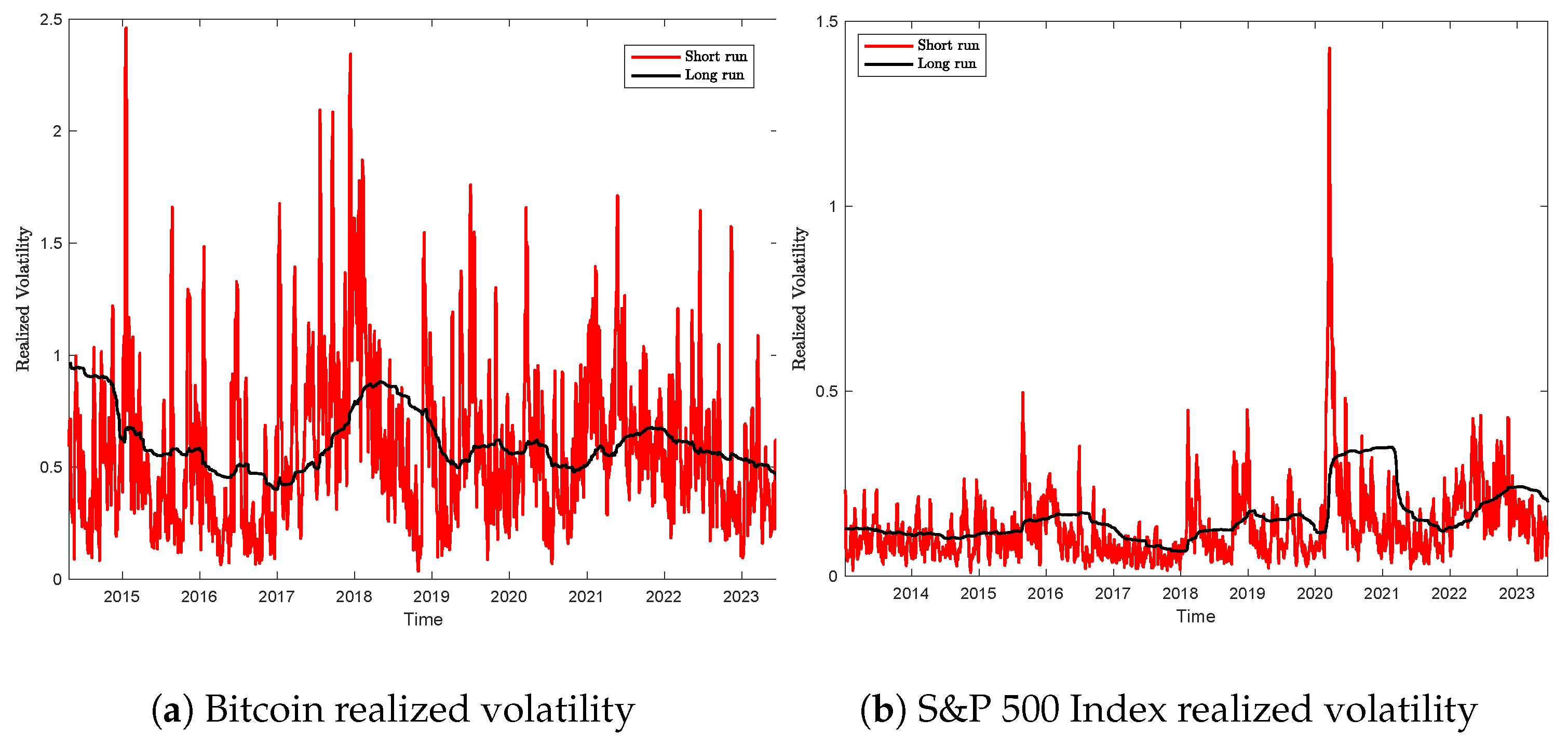
The theoretical statistics and the GTS probability density function are computed based on parameter estimations, and their values are analyzed. The theoretical statistics of Bitcoin and the S&P 500 Index are also compared to the empirical estimations.

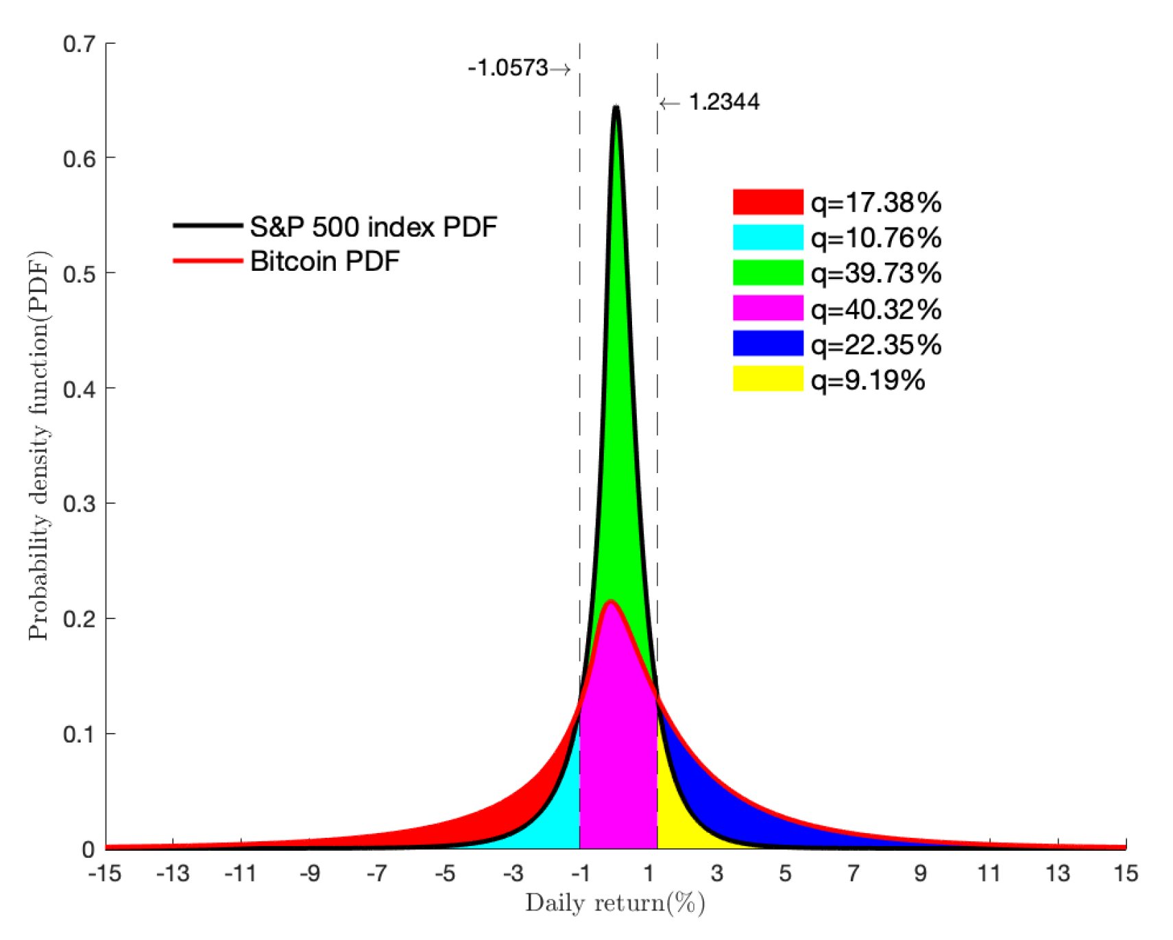
As illustrated in Figure 3, both GTS probability density functions exhibit tail events, which are much more prevalent than we would expect with a Normal distribution. The heavy-tailed distribution captures the huge price swings of Bitcoin and the S&P 500 Index. The theoretical kurtosis statistics are $8.92319$ for S&P 500 returns and $9.74633$ for Bitcoin returns, almost three times the kurtosis of the Normal distribution. Many studies have shown that kurtosis is not a measure of peakedness but rather a measure of tailedness [36,37,38]. The peakedness of the GTS probability density function is another characteristic, as shown in Figure 3. In contrast to the Normal distribution, there is a higher concentration of data values around the mean. The degree of concentration is much higher for S&P 500 returns in Figure 3b than the Bitcoin returns distribution in Figure 3a. Both GTS distributions in Figure 3 are referred to as leptokurtic distributions in the literature.

Figure 3. Probability density functions.

The probability density function of Bitcoin returns is presented in Figure 3a. The Normal probability density (red curve) with mean (${\kappa }_1=0.15\%$) and standard deviation ($\sigma =3.99\%$) is plotted alongside the GTS probability density (black curve). The Normal distribution shows that $35.15\%$ of Bitcoin returns (in purple) are within $-1.57\%$ and $2.07\%$, which is $19.63\%$ lower than the actual percentage of Bitcoin returns. According to statistics, approximately $20.72\%$ of Bitcoin returns (in cyan) are within $-9.53\%$ and $-1.57\%$; against $20.99\%$ within $2.07\%$ and $10.05\%$, on the right side (in yellow). As shown in Figure 3a, the Normal distribution overestimates the probability on both sides (in red and blue).

The probability density function of the S&P 500 Index returns is presented in Figure 3b. The Normal probability density (red curve) with mean (${\kappa }_1=0.04\%$) and standard ($\sigma =1.09\%$) deviations are plotted along with the GTS probability density (black curve). Similar to the previous analysis, the Normal distribution shows that $38.82\%$ of S&P 500 Index returns are concentrated within $-0.43\%$ and $0.68\%$; the percentage is $17.02\%$ lower than the actual percentage of the S&P 500 Index returns. According to statistics, approximately $21.31\%$ of S&P 500 Index returns (in cyan) are within $-2.56\%$ and $-0.43\%$; against $19.49\%$ of S&P 500 Index returns (in yellow), within $0.68\%$ and $2.85\%$. Like Bitcoin returns, the Normal distribution overestimates the probability of the S&P 500 Index returns on both sides (in red and blue).

The GTS probability density functions for S&P 500 Index returns and Bitcoin returns are compared in Figure 4. The heavy-tailedness is the main characteristic of Bitcoin returns, whereas peakedness characterizes the S&P 500 Index.

Figure 4. Bitcoin versus $S\&P$ 500 Index returns.

As shown in Figure 4, only $40.32\%$ of Bitcoin returns (in purple) are within $-1.06\%$ and $1.23\%$. Each tailed distribution of the Bitcoin return is heavier. Actually, $28.14\%$ of Bitcoin returns are less than $-1.06\%$, and $31.54\%$ are more than $1.23\%$. While there is a heavy concentration of the S&P 500 Index returns around the mean, with approximately $80.05\%$ of S&P 500 Index returns within $-1.06\%$ and $1.23\%$; only $10.76\%$ of S&P 500 Index returns (in cyan) are less than $-1.06\%$ and $9.19\%$ are more than $1.23\%$ (in yellow).

The cumulants ($k_k$) of the GTS distribution are stated in Theorem 2, and their formulas produce the theoretical values of the following indicators: means, standard deviation, skewness, and kurtosis. Empirical statistics from the sample data were also estimated, and the results are summarized in Table 5.

Table 5. Summary statistics.

	S&P 500		Bitcoin
Label	Empirical	Theoretical	Empirical	Theoretical
Sample size (m)	3386		3705
Mean (${\kappa }_1$)	0.0401%	0.0401%	0.1488%	0.1489%
Standard deviation ($\sigma =\sqrt{{\kappa }_2}$)	1.1192%	1.0947%	3.9784%	3.9866%
Coefficient of Variation (CV)	27.8892	27.2776	26.7329	26.7732
Skewness ($\frac{{\kappa }_3}{{\kappa }_2^{3/2}}$)	−0.7233	−0.5796	−0.3274	−0.3199
Kurtosis ($3+\frac{{\kappa }_4}{{\kappa }_2^2}$)	16.0464	8.9232	8.8850	9.7463
Max value	8.9683%		28.0520%
Min Value	−12.7652%		−26.6197%

As shown in Table 5, the empirical and theoretical mean (${\kappa }_1$), standard deviation ($\sigma$), and Coefficient of Variation (CV) are consistent for each asset. However, the S&P 500 Index estimation overestimates the kurtosis and skewness statistics. The plausible explanation is the impact of the outliers ($-12.7652\%$, $8.96883\%$).

7. Analysis and Findings: Value-at-Risk and Average Value-at-Risk

Value-at-risk (VaR(X)) and average value-at-risk (AVaR(X)) are widely used financial risk measures. The VaR(X) can be defined as the minimum level of loss or profit at a given confidence level. The estimations of the VaR(X) and AVaR(X) are compared to the empirical $\widehat{VaR}\left(X\right)$ and $\widehat{AVaR}\left(X\right)$.

Consider the sorted sample $x_1,x_2,\dots ,x_n$ corresponding to instant $t_1,t_2,\dots ,t_n$, then the empirical $\widehat{VaR}$ and $\widehat{AVaR}$ at tail probability ($\alpha$) are obtained by applying the following estimators [39,40]:

$${\widehat{VaR}}_{\alpha }=x_{(\lceil n\alpha \rceil )}{\widehat{AVaR}}_{\alpha }=\frac{1}{1-\alpha }\left[\frac{1}{n}\sum _{\lceil n\alpha \rceil +1}^n{x}_j+(\frac{\lceil n\alpha \rceil }{n}-\alpha )x_{(\lceil n\alpha \rceil )}\right],$$

(26)

where the notation $\lceil x\rceil$ stands for the smallest integer larger than x.

7.1. Analysis and Findings: Value-at-Risk ($Va{R}_{\alpha }\left(X\right)$)

Based on the characteristic exponent of the GTS distribution, we develop a methodology to compute the theoretical VaR(X). We assume the return distribution function is continuous. Formally, the VaR(X) at confidence level $(1-\alpha )$ or tail probability ($\alpha$) is the ${\alpha }^{th}$ quantile of the return distribution and has the following mathematical expression:

$$\begin{array}{c}\hfill Va{R}_{\alpha }\left(X\right)=inf\left\{x\right|p(X\le x)\ge \alpha \}=F^{-1}\left(x\right),\end{array}$$

(27)

where $0\le \alpha \le 1$ and $F^{-1}$ is the inverse of the cumulative distribution function.

The GTS($\mu$, ${\beta }_{+}$, ${\beta }_{-}$, ${\alpha }_{+}$, ${\alpha }_{-}$, ${\lambda }_{+}$, ${\lambda }_{-}$) density and cumulative functions do not have closed form, which makes it difficult to estimate the ${\alpha }^{th}$ quantile analytically. Therefore, we rely on the computational method based on the advanced fast FRFT developed previously.

Theorem 3.

Let a probability cumulative function $F\left(x\right)$ be at least four times continuously differentiable and let ${\left(F_j\right)}_{1\le j\le m}$ be a sample of $F\left(x\right)$ on a sequence of evenly spaced input values ${\left(x_j\right)}_{1\le j\le m}$, with $F\left(x_j\right)=F_j$. We also consider $x_{\alpha }$, a ${\alpha }^{th}$ quantile defined by $F\left(x_{\alpha }\right)=\alpha$, with $x_i<x_{\alpha }<x_{i+1}$ and $F_i<F\left(x_{\alpha }\right)<F_{i+1}$.

There exists a unique value, $y\in (0,1)$, and $b_0$, $b_1$, $b_2$, $b_3$, $b_4$ coefficients such that y is a solution of the polynomial equation of degree 4 (28).

$$b_0+b_{1}y+b_2{y}^2+b_3{y}^3+b_4{y}^4=0$$

(28)

The ${\alpha }^{th}$ quantile ($x_{\alpha }$) can be written as follows:

$$x_{\alpha }=x_i+y(x_{i+1}-x_i).$$

(29)

Proof. 

The Taylor series approximation can be applied to the four-times continuously differentiable function $F\left(x\right)$, and we have the following results:

$$\begin{array}{cc}\hfill F\left(x_{\alpha }\right)& =F_i+\frac{u}{1!}{F}_i^{\left(1\right)}+\frac{u^2}{2!}{F}_i^{\left(2\right)}+\frac{u^3}{3!}{F}_i^{\left(3\right)}+\frac{u^4}{4!}{F}_i^{\left(4\right)}+O\left(u^4\right)\hfill \\ \hfill u& =x_{\alpha }-x_i,\underset{u\to 0}{lim}O\left(u^4\right)=0\hfill \end{array},$$

(30)

where $F_i^{\left(1\right)}$, $F_i^{\left(2\right)}$, $F_i^{\left(3\right)}$, and $F_i^{\left(4\right)}$ are determined by the central difference representations [41] of $O\left({\Delta }^2\right)$ with $\Delta =x_{i+1}-x_i$.

$$\begin{array}{cc}\hfill a_1& =\Delta F_i^{\left(1\right)}=\frac{-F_{i-1}+F_{i+1}}{2}\hfill \\ \hfill a_2& ={\Delta }^2{F}_i^{\left(2\right)}=F_{i-1}-2F_i+F_{i+1}\hfill \\ \hfill a_3& ={\Delta }^3{F}_i^{\left(3\right)}=\frac{-F_{i-2}+2F_{i-1}-2F_{i+1}+F_{i+2}}{2}\hfill \\ \hfill a_4& ={\Delta }^4{F}_i^{\left(4\right)}=F_{i-2}-4F_{i-1}+6F_i-4F_{i+1}+F_{i+2}\hfill \end{array}$$

(31)

By removing the function $O\left({\Delta }^4\right)$ in (30), we have the polynomial equation as follows:

$$\begin{array}{c}\hfill -(\alpha -F_i)+a_1\frac{x_{\alpha }-x_i}{x_{i+1}-x_i}+\frac{a_2}{2!}{\left(\frac{x_{\alpha }-x_i}{x_{i+1}-x_i}\right)}^2+\frac{a_3}{3!}{\left(\frac{x_{\alpha }-x_i}{x_{i+1}-x_i}\right)}^3+\frac{a_4}{4!}{\left(\frac{x_{\alpha }-x_i}{x_{i+1}-x_i}\right)}^4=0\end{array}.$$

Let us take $y=\frac{x_{\alpha }-x_i}{x_{i+1}-x_i}$, $b_0=-(\alpha -F_i)$, $b_1=a_1$, $b_2=\frac{a_2}{2!}$, $b_3=\frac{a_3}{3!}$, $b_4=\frac{a_4}{4!}$.

The polynomial equation becomes:

$$b_0+b_{1}y+b_2{y}^2+b_3{y}^3+b_4{y}^4=0.$$

(32)

Let us have $f\left(y\right)=b_0+b_{1}y+b_2{y}^2+b_3{y}^3+b_4{y}^4$. $f\left(y\right)$ is a continuous function with $f\left(0\right)=b_0=-(\alpha -F_i)<0$ and $f\left(1\right)=b_0+b_1+b_2+b_3+b_4>0$. In fact, We have $F_i<\alpha <F_{i+1}$ and $\alpha =\lambda F_i+(1-\lambda )F_{i+1}$ with $0<\lambda <1$.

$$\begin{array}{cc}\hfill & f\left(1\right)=b_0+b_1+b_2+b_3+b_4\hfill \\ \hfill & =\frac{1}{4!}\left[(F_i-F_{i-2})-5(\alpha -F_i)+16(F_{i+1}-\alpha )+3(F_{i+2}-\alpha )\right]\hfill \\ \hfill & =\frac{1}{4!}\left[(F_{i-1}-F_{i-2})+(F_i-F_{i-1})+(24\lambda -5)(F_{i+1}-F_i)+3(F_{i+2}-F_{i+1})\right]\hfill \end{array}$$

(33)

We have $f\left(1\right)>0$ because the cumulative function $F\left(x\right)$ is an increasing function at an increasing rate followed by a decreasing rate. The mean-value theorem guarantees the existence of the solution $\left(y\right)$ over the interval (0,1). $f\left(y\right)$ is an increasing function over the interval $(0,1)$. Therefore, y is a unique value over $(0,1)$.

Given a root (y) of Equation (32) with $0<y<1$, we have the estimation of the ${\alpha }^{th}$ quantile as follows:

$$x_{\alpha }=x_i+y(x_{i+1}-x_i).$$

□

As shown in Figure 4 and Table 5, the GTS distribution generated from Bitcoin and S&P 500 Index returns are not symmetric. Therefore, for a given tail probability ($\alpha$), the $Va{R}_{\alpha }\left(X\right)$ is not expected to yield the same value as the $Va{R}_{1-\alpha }\left(X\right)$ for a confidence level ($1-\alpha$). For tail probability ($\alpha$) from $0.5\%$, $1\%$,…, $10\%$, the theoretical and empirical $Va{R}_{\alpha }\left(X\right)$ was computed and is summarized in Table A1 (Appendix A). For the corresponding confidence level ($1-\alpha$) from $90\%$,…,$99\%$, $99.5\%$, the theoretical and empirical ($Va{R}_{1-\alpha }\left(X\right)$) are summarized in Table 6. Both tables show that the empirical and theoretical $VaR\left(X\right)$ is consistent. As expected, Bitcoin’s theoretical and empirical $Va{R}_{1-\alpha }\left(X\right)$ are higher than that of the S&P 500 Index, which is consistent with the heavy-tailedness of Bitcoin returns. We have the same pattern in Table A1.

Table 6. Value-at-risk statistics for profit values.

${\mathit{VaR}}_{1-\mathit{\alpha }}\left(\mathit{X}\right)$	S&P 500 Index (%)		Bitcoin (%)
Confidence Level ($\mathbf{1}-\mathit{\alpha }$)	Empirical	Theoretical	Empirical	Theoretical
$90\%$	1.1819	1.1760	4.3173	4.2392
$91\%$	1.2638	1.2499	4.5631	4.5379
$92\%$	1.3311	1.3333	4.8620	4.8761
$93\%$	1.4050	1.4288	5.1729	5.2647
$94\%$	1.4770	1.5402	5.5775	5.7202
$95\%$	1.5939	1.6738	6.3628	6.2679
$96\%$	1.7231	1.8399	7.1021	6.9508
$97\%$	1.9259	2.0583	7.9802	7.8507
$98\%$	2.2504	2.3738	9.5034	9.1534
$99\%$	2.8115	2.9334	11.1161	11.4653
$99.5\%$	3.3713	3.5166	13.5660	13.8771

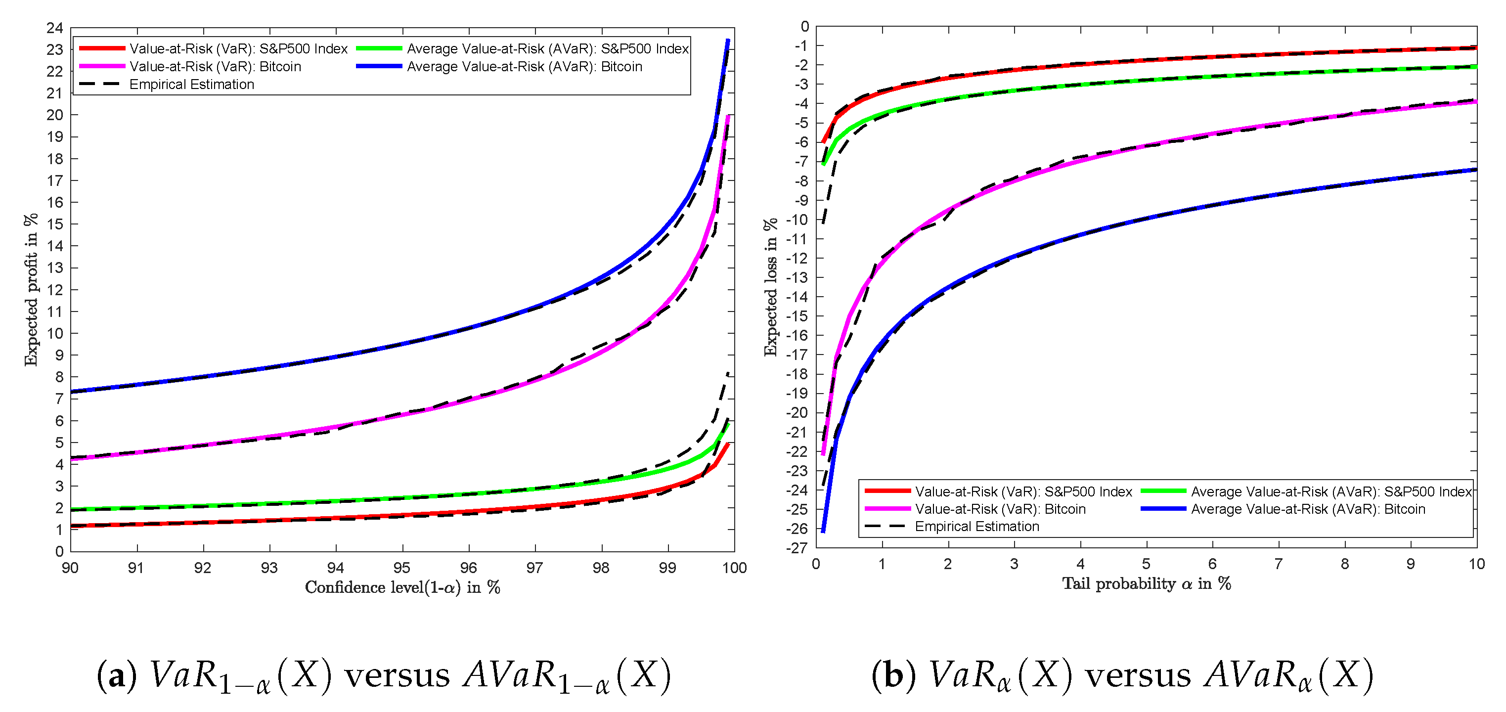
As shown in Table 6, the 95% $Va{R}_{1-\alpha }\left(X\right)$ of both the S&P 500 Index and Bitcoin are equal to $3.52\%$ and $13.88\%$, respectively. Bitcoin gains more than 13.88% of its present value with a probability of $5\%$, whereas the S&P 500 Index gains only $3.52\%$ with the same probability. As it is also illustrated in Figure 6, the $Va{R}_{1-\alpha }\left(X\right)$ increases at an increasing rate in Figure 6a, and $Va{R}_{\alpha }\left(X\right)$ increases at a decreasing rate in Figure 6b. There is also a discrepancy between the $Va{R}_{\alpha }\left(X\right)$ of Bitcoin and the S&P 500 Index. VaR(X) does not provide any information about the magnitude of the losses or profits larger than the VaR(X) level. This is a disadvantage of the VaR(X) indicator [40].

7.2. Analysis and Findings: Average Value-at-Risk ($AVa{R}_{\alpha }\left(X\right)$)

The average value-at-risk ($AVa{R}_{\alpha }\left(X\right)$) at tail probability $\alpha$ is defined as the average of the value-at-risks that are larger than the VaR(X) at tail probability $\alpha$. The mathematical expression can be written as follows:

$$AVa{R}_{\alpha }\left(X\right)=\frac{1}{\alpha }{\int }_0^{\alpha }Va{R}_y\left(X\right)dy.$$

(34)

The GTS distribution is a continuous variable (X), $Va{R}_{\alpha }\left(X\right)=F_X^{-1}\left(\alpha \right)$ in (27) and the integral in (34) becomes

$$\begin{array}{c}\hfill {\int }_0^{\alpha }Va{R}_y\left(X\right)dy={\int }_0^{\alpha }{F}_X^{-1}\left(y\right)dy={\int }_0^{F_X^{-1}\left(\alpha \right)}\theta d{F}_X\left(\theta \right)=E\left[X{1}_{\{X\le Va{R}_{\mathbf{\alpha }}\left(X\right)\}}\right].\end{array}$$

(35)

The average value-at-risk (34) becomes

$$\begin{array}{cc}\hfill AVa{R}_{\alpha }\left(X\right)& =\frac{1}{\alpha }E\left[X{1}_{\{X\le Va{R}_{\mathbf{\alpha }}\left(X\right)\}}\right]\hfill \\ \hfill & =\frac{1}{\alpha }E\left[Va{R}_{\alpha }\left(X\right)1_{\{X\le Va{R}_{\mathbf{\alpha }}\left(X\right)\}}+{\left(X-Va{R}_{\mathbf{\alpha }}\left(X\right)\right)}^{-}\right]\hfill \\ \hfill & =Va{R}_{\alpha }\left(X\right)+\frac{1}{\alpha }E\left[{\left(X-Va{R}_{\alpha }\left(X\right)\right)}^{-}\right]\hfill \end{array}.$$

(36)

For the confidence level $(1-\alpha )$, $AVa{R}_{1-\alpha }$ becomes

$$\begin{array}{cc}\hfill AVa{R}_{1-\alpha }\left(X\right)& =\frac{1}{1-\alpha }{\int }_0^{1-\alpha }Va{R}_{1-y}\left(X\right)dy=\frac{1}{1-\alpha }{\int }_{\alpha }^{1}Va{R}_y\left(X\right)dy\hfill \\ \hfill & =Va{R}_{1-\alpha }\left(X\right)+\frac{1}{1-\alpha }E\left[{\left(X-Va{R}_{1-\alpha }\left(X\right)\right)}^{+}\right]\hfill \end{array}.$$

(37)

We have the following expression on the loss ($\alpha \le \frac{1}{2}$) and the profit ($\alpha \ge \frac{1}{2}$) of the returns distribution:

$$\begin{array}{ccc}\hfill AVa{R}_{\alpha }\left(X\right)& =Va{R}_{\alpha }\left(X\right)+\frac{1}{\alpha }E\left[{\left(X-Va{R}_{\alpha }\left(X\right)\right)}^{-}\right],\hfill & \hfill \alpha <\frac{1}{2}\\ \hfill AVa{R}_{1-\alpha }\left(X\right)& =Va{R}_{1-\alpha }\left(X\right)+\frac{1}{1-\alpha }E\left[{\left(X-Va{R}_{1-\alpha }\left(X\right)\right)}^{+}\right],\hfill & \hfill \alpha >\frac{1}{2}\end{array}.$$

(38)

Theorem 4.

Let $k\in \mathbb{R}$. X is a GTS($\mu$,${\beta }_{+}$,${\beta }_{-}$,${\alpha }_{+}$,${\alpha }_{-}$,${\lambda }_{+}$,${\lambda }_{-}$) random variable with characteristic exponent function $\Psi \left(\xi \right)$.

There exists $q>0$ such that

$$\begin{array}{cc}\hfill E\left[{\left(X-k\right)}^{+}\right]& =\frac{1}{2\pi }{\int }_{-\infty +iq}^{+\infty +iq}\frac{-1}{z^2}{e}^{izk+\Psi (-z)}dz\hfill \\ \hfill E\left[{\left(X-k\right)}^{-}\right]& =\frac{1}{2\pi }{\int }_{-\infty -iq}^{+\infty -iq}\frac{1}{z^2}{e}^{izk+\Psi (-z)}dz\hfill \end{array}.$$

(39)

Proof. 

$g(X,k)={(X-k)}^{+}$ is the payoff of the call option, and the Fourier transform of g is derived as follows:

$$\begin{array}{cc}\hfill \mathcal{F}\left[g\right](y,k)& ={\int }_{-\infty }^{+\infty }{e}^{-iyx}g(x,k)dx={\int }_{-\infty }^{+\infty }{e}^{-iyx}{(x-k)}^{+}dx\hfill \\ \hfill & ={\int }_k^{+\infty }{e}^{-iyx}(x-k)dx\hfill \\ \hfill & ={\left[\frac{1+(x-k)iy}{y^2}{e}^{-iyx}\right]}_k^{+\infty }=-\frac{1}{y^2}{e}^{-iyk}\mathrm{for}\Im \left(y\right)<0\hfill \end{array},$$

(40)

where $\Im \left(y\right)$ is the imaginary of y.

Similarly, $g(X,k)={(X-k)}^{-}$ is the payoff of the put option, and the Fourier transform becomes

$$\mathcal{F}\left[g\right](y,k)={\left[\frac{1+(x-k)iy}{y^2}{e}^{-iyx}\right]}_{-\infty }^k=\frac{1}{y^2}{e}^{-iyk}\mathrm{for}\Im \left(y\right)>0.$$

(41)

The call payoff (39) can be recovered from the inverse of Fourier if there exists $q>0$ such that

$$\begin{array}{c}\hfill \check{g}(x,k)=\frac{1}{2\pi }{\int }_{-\infty +iq}^{+\infty +iq}{e}^{iyx}\mathcal{F}\left[g\right](y,k)dy=-\frac{1}{2\pi }{\int }_{-\infty +iq}^{+\infty +iq}\frac{1}{y^2}{e}^{iy(x-k)}dy.\end{array}$$

(42)

We have the following expression:

$$\begin{array}{cc}\hfill E\left[{\left(X-k\right)}^{+}\right]& ={\int }_{-\infty }^{+\infty }g(y,k)f\left(y\right)dy\hfill \\ \hfill & =\frac{1}{2\pi }{\int }_{-\infty }^{+\infty }{\int }_{-\infty }^{+\infty }{e}^{-iyz+\Psi \left(z\right)}g(y,k)dydzwhereg(y,k)={(y-k)}^{+}\hfill \\ \hfill & =\frac{1}{2\pi }{\int }_{-\infty }^{+\infty }{e}^{\Psi \left(z\right)}{\int }_{-\infty }^{+\infty }{e}^{-iyz}g(y,k)dydz\hfill \\ \hfill & =\frac{1}{2\pi }{\int }_{-\infty -iq}^{+\infty -iq}{e}^{\Psi \left(z\right)}\mathcal{F}\left[g\right](z,k)dz\mathrm{recall}(40)\hfill \\ \hfill & =-\frac{1}{2\pi }{\int }_{-\infty -iq}^{+\infty -iq}\frac{1}{z^2}{e}^{-izk+\Psi \left(z\right)}dz=\frac{1}{2\pi }{\int }_{-\infty +iq}^{+\infty +iq}\frac{-1}{z^2}{e}^{izk+\Psi (-z)}dz\hfill \end{array}$$

The same development holds for $E\left[{\left(X-k\right)}^{-}\right]$. □

The error function $ER(k,q)$ between the call payoff and the inverse Fourier (42) is defined as follows:

$$\begin{array}{c}\hfill ER(k,q)=\sqrt{\frac{1}{m}\sum _{j=1}^m{\left[{(x_j-k)}^{+}-\check{g}(x_j,k)\right]}^2}\mathrm{with}-M\le x_j\le M,M>0,\end{array}$$

(43)

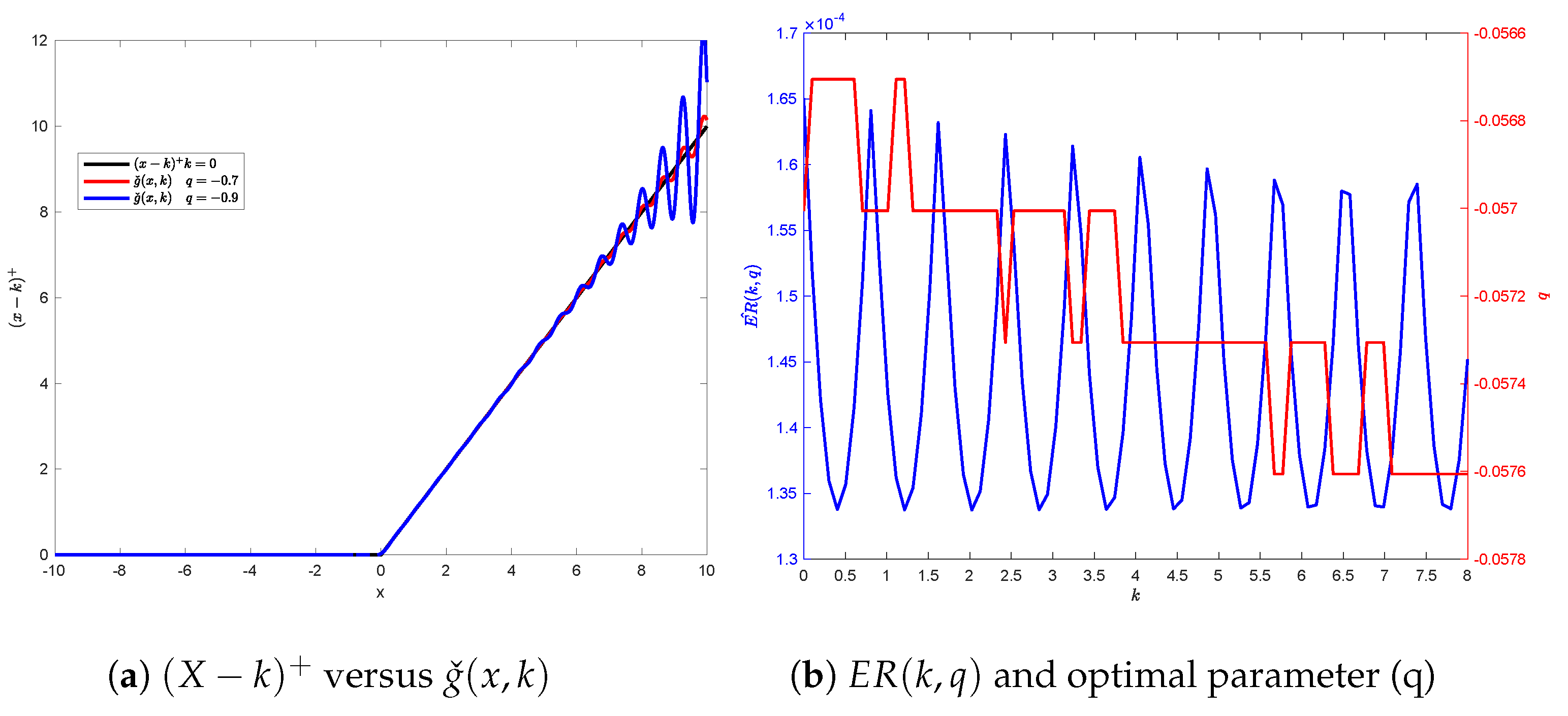
where k (strike price) and q (parameter) are the inputs of the function $ER(k,q)$; the parameter q is used to optimize the function $ER(k,q)$. Figure 5a shows how the accuracy of the inverse Fourier (42) depends on the parameter q.

Figure 5. Optimal parameter (q) and minimum error value ($ER(k,q)$).

Figure 5b displays the $ER(k,q)$ minimum value (in blue) as a function of the strike price (k). The corresponding optimal parameter (q) is graphed as a function of the strike price (k) in Figure 5b. The $ER(k,q)$ minimum value oscillates between $1.337\ast {10}^{-4}$ and $1.650\ast {10}^{-4}$, which is almost zero. The optimal parameter (q) decreases slowly from $-0.0576$ to $-0.0567$, as shown Figure 5b.

Corollary 1.

X is a GTS($\mu$,${\beta }_{+}$,${\beta }_{-}$,${\alpha }_{+}$,${\alpha }_{-}$,${\lambda }_{+}$,${\lambda }_{-}$) random variable with characteristic exponent function $\Psi \left(\xi \right)$.

There exists $q>0$, such that

$$\begin{array}{c}\hfill AVa{R}_{1-\alpha }\left(X\right)=Va{R}_{1-\alpha }\left(X\right)+\frac{1}{1-\alpha }\frac{1}{2\pi }{\int }_{-\infty +iq}^{+\infty +iq}\frac{-1}{z^2}{e}^{izVa{R}_{1-\alpha }\left(X\right)+\Psi (-z)}dz\\ \hfill AVa{R}_{\alpha }\left(X\right)=Va{R}_{\alpha }\left(X\right)+\frac{1}{\alpha }\frac{1}{2\pi }{\int }_{-\infty -iq}^{+\infty -iq}\frac{1}{z^2}{e}^{izVa{R}_{\alpha }\left(X\right)+\Psi (-z)}dz\end{array}.$$

(44)

Proof. 

Equation (38) leads to Equation (44) by substituting $k=Va{R}_{\alpha }\left(X\right)$ and applying Theorem (4). □

For tail probability ($\alpha$) from $0.5\%$, $1\%$,…, $10\%$, the theoretical and empirical average value-at-risk ($AVa{R}_{\alpha }\left(X\right)$) was computed and summarized in Table A2 (Appendix A). For the corresponding confidence Level ($1-\alpha$) from $90\%$,…, $99\%$, $99.5\%$, the theoretical and empirical $AVa{R}_{1-\alpha }\left(X\right)$ are summarized in Table 7. Both tables show consistent empirical and theoretical AVaR(X). As expected, Bitcoin’s theoretical and empirical $AVaR\left(X\right)$ are higher than that of the S&P 500 Index, which is consistent with the heavy-tailedness of Bitcoin.

Table 7. Average value-at-risk statistics for profit values.

${\mathit{AVaR}}_{1-\mathit{\alpha }}\left(\mathit{X}\right)$	S&P 500 (%)		Bitcoin (%)
Confidence Level ($\mathit{\alpha }$)	Empirical	Theoretical	Empirical	Theoretical
$90\%$	1.8976	1.9278	7.3077	7.3190
$91\%$	1.9730	2.0074	7.6273	7.6451
$92\%$	2.0584	2.0971	7.9916	8.0130
$93\%$	2.1585	2.1997	8.4150	8.4343
$94\%$	2.2790	2.3193	8.9274	8.9259
$95\%$	2.4304	2.4624	9.5154	9.5145
$96\%$	2.6269	2.6399	10.2239	10.2448
$97\%$	2.8887	2.8724	11.1451	11.2015
$98\%$	3.3001	3.2070	12.3666	12.5767
$99\%$	4.1403	3.7960	14.5488	14.9924
$99.5\%$	5.2054	4.4047	16.9509	17.4790

To generalize the computation performed in Table 7 and Table A2 and accounting for a large range of values, we consider the interval $[0,10]$ for tail probability ($\alpha$) in Figure 6b and the interval $[90,100]$ for confidence level ($1-\alpha$) in Figure 6a. As illustrated in Figure 6a, the $AVa{R}_{1-\alpha }\left(X\right)$ of Bitcoin and the S&P 500 Index increase at an increasing rate, which justified the concave nature of each curve.

Figure 6. Value-at-risk (VaR) versus Average value-at-risk (AVaR).

From Figure 6a, the $AVa{R}_{1-0.999}\left(X\right)=23.48\%$ for Bitcoin and $AVa{R}_{1-0.999}\left(X\right)=5.88\%$ for the S&P 500 Index, while for the tail probability ($\alpha$) in Figure 6b, the $AVa{R}_{0.001}\left(X\right)=-26.21\%$ for Bitcoin and $AVa{R}_{0.001}\left(X\right)=-7.18\%$ for the S&P 500 Index.

As shown in Figure 6, at a $\alpha$ risk level, the severity of the loss ($AVa{R}_{\alpha }\left(X\right)$) on the left side of the distribution is larger than the severity of the profit ($AVa{R}_{1-\alpha }\left(X\right)$) on the right side of the distribution. The left-skewed nature of the distribution provides some explanation.

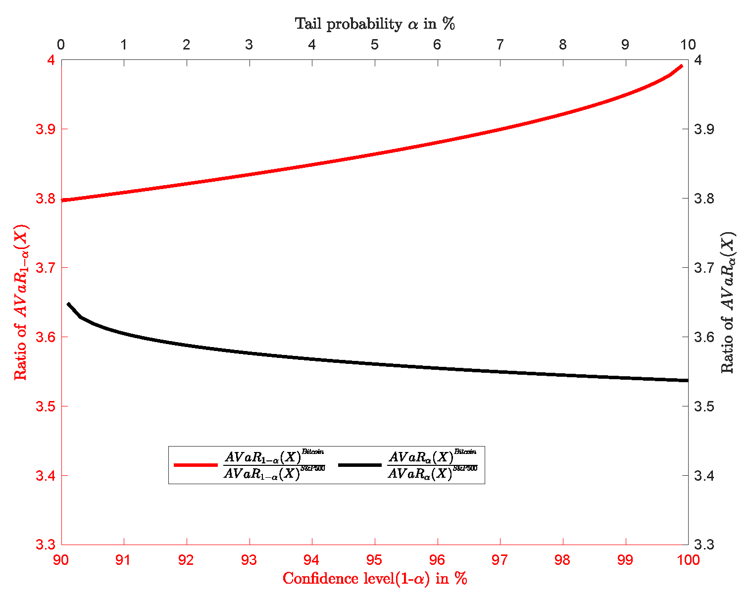
The magnitude of the discrepancy between the $AVa{R}_{\alpha }\left(X\right)$ of Bitcoin and S&P 500 Index can be evaluated by assessing the ratio of the $AVa{R}_{\alpha }\left(X\right)$ of Bitcoin to the $AVa{R}_{\alpha }\left(X\right)$ of the S&P 500 Index. The relationship is depicted in Figure 7.

Figure 7. $\frac{{{\mathit{AVaR}}_{\alpha }\left(X\right)}^{Bitcoin}}{{{\mathit{AVaR}}_{\alpha }\left(X\right)}^{S\&P500}}$.

The profits (in red) generated by the $AVa{R}_{1-\alpha }\left(X\right)$ of Bitcoin at one significant figure is four times larger than that of the S&P 500 Index. Similarly, the losses (in black) generated by the $AVa{R}_{\alpha }\left(X\right)$ of Bitcoin at one significant figure is four times larger than that of the S&P 500 Index, as shown in Figure 7.

8. Conclusions

The paper analyzes the daily return distributions of Bitcoin and the S&P 500 Index. It assesses their tail probabilities through the value-at-risk (VaR(X)) and the average value-at-risk (AVaR(X)). As a methodology, we use the historical prices for Bitcoin and the S&P 500 Index. Bitcoin price spans from 04 January 2010 to 16 June 2023, while the S&P 500 Index price spans from 28 April 2013 to 22 June 2023. Each historical data fits the seven-parameter General Tempered Stable (GTS) distribution to the underlying data return distribution. The advanced fast FRFT scheme is developed from the classic fast FRFT algorithm and the 12-point composite Newton–Cotes rule. The advanced fast FRFT scheme is used to perform the maximum likelihood estimation of seven parameters of the GTS distribution. It results from the GTS distribution fitting that the stability indexes, the process intensities, and the decay rate are all positive. Bitcoin and S&P 500 Index returns are infinite activity and finite variance processes. The parameter analysis shows that Bitcoin and S&P 500 Index returns are left-skewed distributions. The study of the probability density functions and some key statistics show that the tail events of Bitcoin and the S&P 500 Index are much more prevalent than we would expect from a Normal distribution. Both probability density functions are leptokurtic distributions. However, the heavy-tailedness is the main characteristic of the Bitcoin returns, whereas the peakedness is the main characteristic of the S&P 500 Index returns. The GTS distribution shows that $80.05\%$ of S&P 500 returns are within $-1.06\%$ and $1.23\%$, against only $40.32\%$ of Bitcoin returns. The value-at-risk and the average value-at-risk reveal significant differences in tail probability between Bitcoin and S&P 500 Index returns. At a risk level ($\alpha$), the severity of the loss ($AVa{R}_{\alpha }\left(X\right)$) on the left side of the distribution is larger than the severity of the profit ($AVa{R}_{1-\alpha }\left(X\right)$) on the right side of the distribution. Compared to the S&P 500 Index, Bitcoin has $39.73\%$ more prevalence to produce high daily returns (more than $1.23\%$ or less than $-1.06\%$). The severity analysis shows that at a risk level ($\alpha$), the average value-at-risk of Bitcoin returns at one significant figure is four times larger than that of the S&P 500 Index returns at the same risk.