Analytical Solutions of Systems of Linear Delay Differential Equations by the Laplace Transform: Featuring Limit Cycles

Abstract

In this paper we develop an approach for obtaining the solutions to systems of linear retarded and neutral delay differential equations. Our analytical approach is based on the Laplace transform, inverse Laplace transform and the Cauchy residue theorem. The obtained solutions have the form of infinite non-harmonic Fourier series. The main advantage of the proposed approach is the closed-form of the solutions, which are capable of accurately evaluating the solution at any time. Moreover, it allows one to study the asymptotic behavior of the solutions. A remarkable discovery, which to the best of our knowledge has never been presented in the literature, is that there are some particular linear systems of both retarded and neutral delay differential equations for which the solution asymptotically approaches a limit cycle. The well-known method of steps in many cases is unable to obtain the asymptotic behavior of the solution and would most likely fail to detect such cycles. Examples illustrating the Laplace transform method for linear systems of DDEs are presented and discussed. These examples are designed to facilitate a discussion on how the spectral properties of the matrices determine the manner in which one proceeds and how they impact the behavior of the solution. Comparisons with the exact solution provided by the method of steps are presented. Finally, we should mention that the solutions generated by the Laplace transform are, in most instances, extremely accurate even when the truncated series is limited to only a handful of terms and in many cases become more accurate as the independent variable increases.

1. Introduction

Time delays appear in many systems and applications. The main aspect to consider in these systems is that the output depends on inputs to the system at previous times [1]. Differential equations that contain time delay effects are called delay differential equations (DDEs). In these equations the derivative of the state variables depend on the state variables or even on the time derivatives at previous times. Applications of DDEs appear in many different fields such as applied mathematics, physics, epidemiology and engineering [2,3,4,5,6,7,8,9,10]. Retarded DDEs (RDDEs) are equations where the time delay only appears in the state variable. Neutral DDEs (NDDEs) are equations where the time delays appear in both the state variables and their time derivatives. Overall, DDEs have a higher degree of complexity than ordinary differential equations (ODEs). A system may become unstable due to the time delay, and periodic solutions may then develop [9,11]. In particular in this article we deal with systems of linear RDDEs and NDDEs. There are many applications of these systems to real world problems. For instance, systems of NDDEs arise when modeling circuits that include delayed elements [12]. More specifically, they include circuits related to transmission lines and partial element equivalent circuits [12]. Another area where linear DDEs arise is in micro electro mechanical systems (MEMS) [13].

The development of techniques for discovering analytical or numerical solutions of DDEs has been the subject of numerous investigations [5,14,15,16,17,18,19,20,21,22,23]. For instance, in [24], a numerical method based on finite differences was developed for solving linear first order NDDEs. In [25], the authors numerically solved linear fractional DDEs using the Chelyshkov matrix method. Another interesting work is presented in [26]. The authors developed a block multistep method to deal with the propagation of derivatives discontinuities in NDDEs. The numerical approach adapted the block multistep method with the Runge–Kutta Fehlberg variable step strategy to find the solution. A recent work developed a numerical methodology to solve non-autonomous linear DDEs [27]. The methodology is based on the use of a spectral discretization of the delayed part to transform the original problem into a matrix linear ODE and then is solved by numerical integrators based on the Magnus expansion.

The method of steps (MoS) is a traditional approach, which is frequently used to obtain the analytical solution of DDEs [9,28,29,30]. This approach produces a piecewise analytical solution that is exact. However, because of the expression swell phenomenon, the procedure of stages frequently fails to give the solution after several steps [28,31,32]. As a result, the MoS approach in most instances cannot predict how the solution will behave over a lengthy period of time. DDEs have also been solved using many different numerical methods [19,33,34].

Recently, a variety of linear DDEs have been solved using the Laplace transform (LT) [16,32,35,36]. For instance, in [36], the authors computed solutions that featured resonance for linear DDEs. Furthermore, in [29], the Laplace transform method (LTM) was employed by the authors to look at the stability of linear DDEs. In addition, in [37], the authors used the LT to establish the stabilities of fractional systems of first-order linear differential equations. For systems of DDEs several works have been developed to find the solutions [38,39,40,41,42]. For instance, in [38], the authors developed a mathematical approach for the analytical solution to systems of linear RDDEs using the matrix Lambert function. This approach uses matrix operations and the concept of the exponential of a matrix. However, this approach requires that the coefficient matrices commute. Moreover, as it has been pointed out in [43], this previous approach based on the exponential matrix has some flaws; therefore, it fails to provide an accurate solution. Later, in [41], the authors improved the previous approach based on the exponential of a matrix to solve systems of linear RDDEs, but for the general case where the coefficient matrices do not commute. This method uses the LT to obtain solutions in the form of an infinite series that includes the matrix Lambert function. On the other hand, in [42], the author developed a method based on Galerkin approximations to obtain numerical solutions of nonlinear NDDEs. In [39], the authors developed nonstandard finite difference schemes to obtain numerical solutions to linear systems of RDDEs, with matrices A and B that commute and that, in general, are not simultaneously diagonalizable. Interestingly, this requirement is similar to the one presented in [38] where the approach is analytical instead of numerical. Later on, the authors improved their approach to account for delay systems with non-commuting matrices [40]. Recently, there have been improvements in regard to methods of solving linear RDDEs [44,45,46,47]. For instance, in [44], the authors deal with linear differential systems with a single delay and multiple delays with linear parts given by non-permutable matrices. Some of these studies rely on the exponential matrix or approximations of it. In addition, some of these methods require one to have a piecewise solution in different intervals that depend on the time delays. These works have mainly focused on the existence and uniqueness of the solutions, even though they provide the procedure to compute the solutions.

In this paper, we study and develop a new approach for obtaining the analytical solutions to systems of linear RDDEs and NDDEs. The proposed analytical approach is based on the LT, inverse Laplace transform (ILT) and the Cauchy residue theorem. In some cases we can rely on the Lambert function to compute the poles, which are required for computing the ILT and therefore the solutions. These solutions have the form of an infinite non-harmonic Fourier series. The main advantage of the proposed approach is that the solutions have closed-forms, which are capable of accurately evaluating the solution at any time. In addition, the LT solution is not piecewise, unlike the MoS solution. Furthermore, the methodology enables one to study the asymptotic behavior of the solutions and find, for instance, limit cycles, which are not evident during the early transient dynamics. This is a feature of the richer dynamics that DDEs offer, and that cannot occur for analogous first order systems of linear ordinary differential equations. As a matter of fact, to the best of our knowledge, this has never been presented in the literature before. A key step in the LTM solution process, when it is applied to linear DDEs, is to evaluate the poles of the transformed equation, in the s-space. There are infinitely many poles and different methods can be used to find them [19,32,38,41]. The poles are then used to compute the ILT, by means of the Cauchy residue theorem [48,49]. The resulting solutions are then obtained in the form of an infinite non-harmonic Fourier series [32,50,51,52]. We present a variety of examples illustrating the methodology in order to facilitate a discussion on how the spectral properties affect the approach and the solutions.

The remainder of this paper proceeds as follows. In the next section, we recall some basic definitions for DDEs and the LTM that are necessary to develop the proposed methodology. We present the methodology for solving systems of linear RDDEs and NDDEs with the LTM with a general history. In Section 3, we present numerical results of the implementation of the proposed methodology to systems of linear RDDEs and NDDEs. We evaluate the reliability and accuracy of the solutions generated by the LT using the exact analytical solutions provided by the MoS. Section 4 is devoted to a summary and discussion of our conclusions.

2. Systems of Linear DDEs

In this paper, we are interested in solving the following general system of linear DDEs:

$$\begin{array}{ccc}{y}^{\prime }\left(t\right)=Ay\left(t\right)+By(t-\tau )+C{y}^{\prime }(t-\tau )& ,& t>0,\end{array}$$

(1)

along with the history function $y\left(t\right)=H\left(t\right)$, $t\in [-\tau ,0]$.

Here, $y\left(t\right),H\left(t\right)\in {\mathbb{R}}^n$ and $A,B$ and C are time-invariant $n\times n$ matrices where the delay $\tau$ is a positive constant. The existence and uniqueness of the solution of the linear system (1) has been proved [11,53]. This new approach is based on the LT and the ILT. We shall solve the linear DDE (1) for several different cases. Now, let us start by deriving the LT solution.

2.1. Solving Linear Systems of DDEs by the LTM

Let us denote $\mathcal{L}\left(y\left(t\right)\right)=Y\left(s\right)$. Then it follows that

$$\mathcal{L}\left(y(t-\tau )\right)=e^{-s\tau }Y\left(s\right)+e^{-s\tau }{\int }_{-\tau }^{0}y\left(v\right)e^{-sv}dv$$

(2)

and

$$\mathcal{L}\left(y^{\prime }(t-\tau )\right)=s{e}^{-s\tau }Y\left(s\right)+s{e}^{-s\tau }{\int }_{-\tau }^{0}y\left(v\right)e^{-sv}dv-y(-\tau ).$$

(3)

Then, applying the LT to (1), we obtain the matrix equation

$$Ys-y\left(0\right)=AY+(B+Cs)e^{-s\tau }Y+(B+Cs)e^{-s\tau }{\int }_{-\tau }^{0}y\left(v\right)e^{-sv}dv-Cy(-\tau ),$$

(4)

or

$$(sI-A-(B+Cs)e^{-s\tau })Y=H\left(0\right)+(B+Cs)e^{-s\tau }{\int }_{-\tau }^{0}H\left(v\right)e^{-sv}dv-CH(-\tau ).$$

(5)

The solution of the above equation can be expressed in the form

$$Y=D^{-1}{v}_h,$$

(6)

where

$$D=sI-A-(B+Cs)e^{-s\tau },$$

(7)

and

$$v_h=H\left(0\right)+(B+Cs)e^{-s\tau }{\int }_{-\tau }^{0}H\left(v\right)e^{-sv}dv-CH(-\tau ).$$

(8)

Equation (5) can also be solved via Cramer’s rule, in which case

$$Y_j=\frac{det\left(N_j\right)}{det\left(D\right)},$$

(9)

and $N_j$ is the matrix formed by replacing columnj in D with the vector $v_h.$ If all of the entries in the history vector $H\left(t\right)$ are bounded: $h_1<H\left(t\right)<$$h_2$, and integrable for $t\in (-\tau ,0)$, then it can be shown that any singularities resulting from the integral term in $v_h$ are removable [32]. In that case, all of the relevant poles are determined by the roots of the (characteristic) equation

$$D\left(s\right)=det(sI-A-(B+Cs)e^{-s\tau })=0.$$

(10)

A key step in the LTM solution process, when it is applied to linear DDEs, is to evaluate all of the poles of the transformed equation, in the s-domain. For instance, Maple software is capable of computing these poles, but it relies upon the user providing it with an accurate initial guess. This can be challenging for certain systems, particularly when two or more of the n (infinite) sequences of poles are clustered close together.

2.2. Computation of the Complex Poles

In order to gain some insight into the locus of the poles, we can divide (10) by $s^n$. The resulting approximated characteristic equation,

$$det(I-C{e}^{-s\tau })=0\mathrm{or}det(C-I{e}^{s\tau })=0,$$

(11)

can then be used to obtain estimates for the location of the poles (for $\left|s\right|$large, and $\mathfrak{Im}\left(s\right)>0$). These estimates can then be used as the initial guesses for determining the actual poles. For additional details, we refer the interested reader to previous works [36,54]. Observe that the second equation (above) is essentially an exact match with the eigenvalue equation for $C.$ Assuming that the matrix C is non-singular, with distinct eigenvalues one gets n (infinite) sequences of poles, with approximate locations given by

$$s_{j,k}=\frac{ln\left({\lambda }_j\right)+2k\pi i}{\tau }j\in \mathbb{N},k\in \mathbb{N},$$

(12)

in which ${\lambda }_j$ is the relevant eigenvalue.

Other possibilities exist such as a repeated eigenvalue. Oftentimes, if we have a repeated eigenvalue, then the complex poles will be clustered fairly close together. However, for n small, one can compute the respective sequences of poles (separately) by factoring $D\left(s\right)$. For example, for a $2\times 2$ system, $D\left(s\right)$ can be factored via the quadratic formula as $D\left(s\right)=(e^{-s\tau }-f_1\left(s\right))(e^{-s\tau }-f_2\left(s\right))$. After which, we can determine the relevant sequences of actual poles from the two respective factors. Interestingly, we do have one example (a NDDE featuring a limit cycle) in which the matrix C has a repeated eigenvalue. In this example, however, one can obtain exact formulas for all of the poles. We shall discuss this in further detail in Section 3.2.

There is also a case for which exact expressions for the poles can be found. If $CA+B=0$, then

$$det(sI-A-(B+Cs)e^{-s\tau })=det(sI-A-C(sI-A)e^{-s\tau })=det(sI-A)det(I-C{e}^{-s\tau })$$

(13)

and since this determinant must equal zero at the poles, it follows that

$$r_{j,k}=\frac{ln\left({\lambda }_j\right)+2k\pi i}{\tau },k\in \mathbb{N}$$

(14)

and

$$r_j={\mu }_j,$$

(15)

where the ${\lambda }_j$ and ${\mu }_j$ are the respective eigenvalues of C and A. Note that to distinguish the approximate locations where we use s, we shall switch to r when referencing the actual poles.

Remark 1.

All of these formulas are approximates (or exact expressions) for the locations of the complex poles above the real axis. We know that once we have computed the actual poles and their residues, the corresponding residues for the poles below the real axis are given by their conjugates. As a matter of preference (and efficiency) we account for this, when applying the Cauchy residue theorem by computing two times the real part of the residues above the real axis. It is also worth mentioning that Maple software can solve (10) directly, using the fsolve command with the complex option. A second option enables the user to specify a rectangle in the complex plane, in which the particular root lies. We used this option in conjunction with the formulas for the approximate pole locations, to compute the actual poles. In most of our examples, the relevant do-loop was able to achieve this for all $k\in [2,N]$, with N being the value at which the series solution is truncated.

2.3. Computation of Poles for RDDEs

For a RDDE ($C=0$)

$$\begin{array}{ccc}{y}^{\prime }\left(t\right)=Ay\left(t\right)+By(t-\tau )& ,& t>0,\end{array}$$

(16)

the analogous formulas for the approximate loci of the complex poles (for $\left|s\right|$ large, and $\mathfrak{Im}\left(s\right)>0$) can be obtained from the equation

$$det(Is{e}^{s\tau }-B)=0,$$

(17)

which is essentially an exact match with the eigenvalue equation for $B.$ Assuming the matrix B is non-singular and has distinct eigenvalues, it follows that one gets n (infinite) sequences of poles with approximate loci given by

$$s_{j,k}=\frac{W_k\left(\tau {\lambda }_j\right)}{\tau }j\in \mathbb{N},k\in \mathbb{N},$$

(18)

where $W_k$ denotes the Lambert function [19,55,56,57,58].

However, if the matrices A and B commute, we can obtain exact formulas for all of the poles. If we assume the eigenvalues of B are distinct, then A and B can be diagonalized using the same eigenvectors, in which case

$$\left|sI-A-B{e}^{-s\tau }\right|=\prod _{j=1}^n(s-{\mu }_j-{\lambda }_j{e}^{-s\tau }),$$

(19)

where ${\mu }_j$ and ${\lambda }_j$ are the respective corresponding eigenvalues of A and B.

Therefore, the complete sequence of poles is given by

$$r_{j,k}={\mu }_j+\frac{1}{\tau }{W}_k\left(\tau {\lambda }_j{e}^{-{\mu }_j\tau }\right),j=1,2,\dots ,n.$$

(20)

Let us restrict our brief discussion about the real poles to the case when the coefficient matrices are all $2\times 2.$ The exact number of real roots is determined by the matrix entries/parameters and $\tau$. For NDDEs, there can be at most six, because if all of the matrices were diagonal, then the characteristic equation would be

$$D\left(s\right)=(s-A_{11}-(B_{11}+C_{11}s)e^{-s\tau })(s-A_{22}-(B_{22}+C_{22}s)e^{-s\tau })=0.$$

(21)

And it is possible, although granted unlikely, for both of these factors to have three real roots. For RDDEs, however, there can be at most four. The real poles can be computed by plotting the graph of $D\left(s\right)$ for s real, then using the (approximate) points where the graph intersects the s-axis as the initial guesses for determining the actual poles.

Obviously, other methods can be used to find the poles. Regardless of the method, once the poles have been computed one can apply the Cauchy residue theorem to obtain the solution $y\left(t\right)$. If all of the poles are order one, the residues can be computed using L’Hopital’s rule. If this is how one decides to proceed, then, in conjunction with Cramer’s rule,

$$c_{j,k}={\left.\frac{det\left(N_j\right)}{D^{\prime }\left(s\right)}\right|}_{s=r_{j,k}}.$$

(22)

Thus, for a DDE with M real poles,

$$y_j\left(t\right)=\sum _{m=1}^M{c}_{j,m}{e}^{r_{j,m}t}+2\left[\mathfrak{Re}\sum _{k=1}^{\infty }{c}_{j,k}{e}^{r_{j,k}t}\right],j=1,2,\dots ,n.$$

(23)

where $c_{j,k}$ denotes the residue of the complex pole at $s=r_{j,k}$ and $c_{j,m}$ denotes the residue of the real pole at $s=r_{j,m}$.

We will see in the next section that the solutions generated by the LTM are reliable and valid over the entire time domain. On the other hand, the MoS can rarely produce a solution that is capable of evaluating $y\left(t\right)$ for t large.

3. Examples of Systems of Linear RDDEs and NDDEs

In this section, we present a variety of examples illustrating the implementation of the proposed methodology for obtaining solutions to the linear DDE (1). In particular, we consider examples of systems of first-order linear RDDEs and NDDEs. First, we consider two RDDEs for which we can use the Lambert function to compute the poles. We then consider three additional RDDEs for which the poles must be computed numerically. The fourth example features a system for which the solution approaches a limit cycle, and the final RDDE example involves a system with $3\times 3$ matrices. For NDDEs, we present two examples. First, we consider a system where the solution approaches an equilibrium point. We conclude with an example, for which the solution approaches a limit cycle. For all of the examples, we compute the errors by comparing the LT solution with the analytical solution that is obtained by the MoS.

3.1. Linear RDDEs

In this subsection, we deal with linear systems of the form $y^{\prime }\left(t\right)=Ay\left(t\right)+By(t-\tau )$. We first consider the simple case where the matrix $A=0$.

Example 1.

Consider the following linear system of RDDEs:

$$\begin{array}{cccc}\hfill y^{\prime }\left(t\right)& =\left[\begin{array}{cc}-1& 3\\ 1& -2\end{array}\right]y(t-\tau ),\hfill & & t>0,\hfill \\ \hfill y\left(t\right)& =H\left(t\right)=\left[\begin{array}{c}1\\ 1/2\end{array}\right],\hfill & & t\in [-\tau ,0].\hfill \end{array}$$

(24)

where $\tau =1$ and $y\in {\mathbb{R}}^2$. In this example, the characteristic equation is derived from the following matrix

$$sI-B{e}^{-s\tau }.$$

Taking the determinant of this matrix and setting it to zero, one obtains the characteristic equation

$$s^2+3s{e}^{-s}-e^{-2s}=\left(s-\left(-\frac{3}{2}+\frac{\sqrt{13}}{2}\right)e^{-s}\right)\left(s-\left(-\frac{3}{2}-\frac{\sqrt{13}}{2}\right)e^{-s}\right)=0.$$

In this case, we can obtain exact expressions for the two infinite sequences of poles in terms of the Lambert function. In particular,

$$r_{1,k}=W_k\left(-\frac{3}{2}+\frac{\sqrt{13}}{2}\right),$$

and

$$r_{2,k}=W_k\left(-\frac{3}{2}-\frac{\sqrt{13}}{2}\right).$$

Figure 1 depicts the solution given by the LTM. We also include the graph of the solution in the phase space. In this example the solution becomes unbounded due to the fact that at least one pole has a positive real part, i.e., $\mathfrak{Re}\left(r_{ik}\right)>0$. In Figure 2, we include the graph of the absolute errors. The LT solution is very accurate despite the fact that we only used 50 terms in this example. Notice that the error decreases with time.

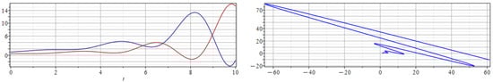
Figure 1. Solution of the linear system of RDDEs (24) over $t\in [0,10\tau ]$ using the LTM (left). The components of the solution are $y_1\left(t\right)$ (blue) and $y_2\left(t\right)$ (red). Solution in the phase space for $t\in [0,14]$ (right).

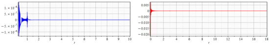
Figure 2. Absolute errors of the solution of the linear system of RDDEs (24) over $t\in [0,10\tau ]$ using LTM. Absolute error for $y_1\left(t\right)$ (left) and $y_2\left(t\right)$ (right).

Example 2.

Consider the following linear system of RDDEs:

$$\begin{array}{cccc}\hfill y^{\prime }\left(t\right)& =\left[\begin{array}{cc}-5& 0\\ 0& -5\end{array}\right]y\left(t\right)+\left[\begin{array}{cc}2& -1\\ -1& 2\end{array}\right]y(t-\tau ),\hfill & & t>0,\hfill \\ \hfill y\left(t\right)& =H\left(t\right)=\left[\begin{array}{c}1\\ 2\end{array}\right],\hfill & & t\in [-\tau ,0].\hfill \end{array}$$

(25)

where $\tau =3$.

In this example we consider a system for which the matrices A and B commute. Recall, that in Section 2 it was shown that when this is the case, we can obtain exact expressions for both sequences of poles, in terms of the Lambert function. Therefore, substituting the eigenvalues of A and B into (20), we find that

$$r_{1,k}=\frac{1}{3}{W}_k\left(9{\mathrm{e}}^{15}\right)-5,$$

and

$$r_{2,k}=\frac{1}{3}{W}_k\left(3{\mathrm{e}}^{15}\right)-5.$$

Figure 3 depicts the exact solution given by the LTM. We also include the graph of the solution in the phase space. The solution approaches the equilibrium point $(0,0)$. This is due to the fact that all the poles have negative real part, i.e., $\mathfrak{Re}\left(r_{j,k}\right)<0$. In Figure 4, we include the graph of the absolute errors. The LT solution is very accurate despite the fact that we only used 50 terms in this example. Notice that the error decreases with time.

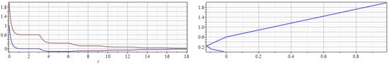
Figure 3. Solution of the linear system of RDDEs (25) over $t\in [0,10\tau ]$ using the LTM (left). The components of the solution are $y_1\left(t\right)$ (blue) and $y_2\left(t\right)$ (red). Solution in the phase space for $t\in [0,20]$ (right).

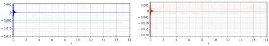
Figure 4. Absolute errors of the solution of the linear system of RDDEs (25) over $t\in [0,10\tau ]$ using LTM. For $y_1\left(t\right)$ on the (left) and $y_2\left(t\right)$ on the (right).

Example 3.

Consider the following linear system of RDDEs:

$$\begin{array}{cccc}\hfill y^{\prime }\left(t\right)& =\left[\begin{array}{cc}-1& -2\\ -1& -2\end{array}\right]y\left(t\right)+\left[\begin{array}{cc}-3/2& 0\\ -2& -1\end{array}\right]y(t-2),\hfill & & t>0,\hfill \\ \hfill y\left(t\right)& =H\left(t\right)=\left[\begin{array}{c}2-t/2\\ 2t+3\end{array}\right],\hfill & & t\in [-2,0].\hfill \end{array}$$

(26)

In this example we consider a system where the matrices A and B do not commute. Recall, as mentioned in Section 2, that when this is the case, we cannot obtain exact expressions for both sequences of poles. We can, however, use the formulas given by (18) to obtain estimates for the locus of the two infinite sequences of poles in terms of the Lambert function. These approximates are given by

$$s_{1,k}={\displaystyle \frac{1}{2}}{W}_k\left(-2\right),$$

and

$$s_{2,k}={\displaystyle \frac{1}{2}}{W}_k\left(-3\right).$$

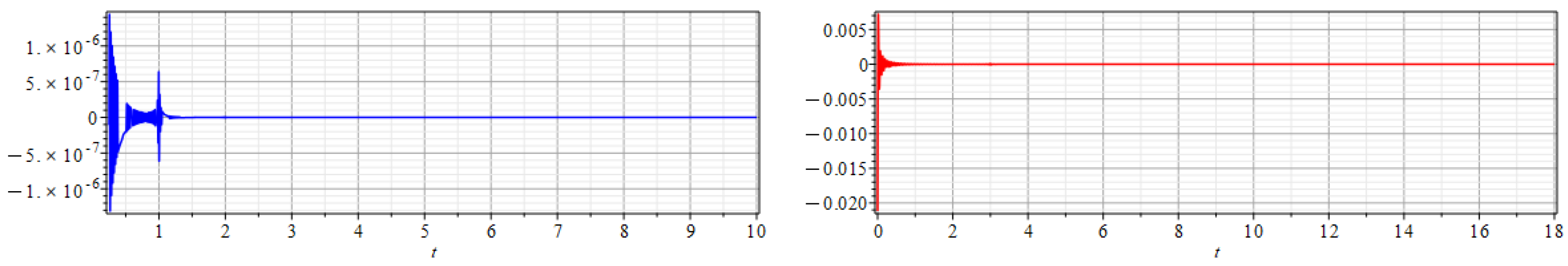
Figure 5 depicts a contour plot (in the complex plane) of the magnitude of $D\left(s\right)$, in which the actual poles lie within the closed blue curves. The sequence of red dots indicate the approximate locations of the poles given by (18). Figure 6 depicts the exact solution given by the LT solution. We also include the graph of the solution in the phase space. The solution approaches an equilibrium point. In Figure 7, we include the graph of the absolute errors. Even though we truncated the series in this example at $N=20$, the LT solution is highly precise.

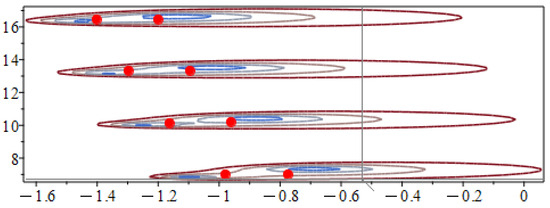
Figure 5. Sequence of poles in the complex plane for the linear system of RDDEs (26).

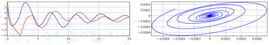
Figure 6. Solution of the linear system of RDDEs (26) over $t\in [0,10\tau ]$ using the LTM (left). The components of the solution are $y_1\left(t\right)$ (blue) and $y_2\left(t\right)$ (red). Solution in the phase space for $t\in [90,200]$ (right).

Figure 7. Absolute errors of the solution of the linear system of RDDEs (26) over $t\in [0,10]$ using LTM. For $y_1\left(t\right)$ on the (left) and $y_2\left(t\right)$ on the (right).

Example 4.

Consider the following linear system of RDDEs:

$$\begin{array}{cccc}\hfill y^{\prime }\left(t\right)& =\left[\begin{array}{cc}-3& w_1\\ 0& w_2\end{array}\right]y\left(t\right)+\left[\begin{array}{cc}0& -\pi \\ \pi & 0\end{array}\right]y(t-\tau ),\hfill & & t>0,\hfill \\ \hfill y\left(t\right)& =H\left(t\right)=\left[\begin{array}{c}8\\ 0\end{array}\right],\hfill & & t\in [-\tau ,0].\hfill \end{array}$$

(27)

where $w_1=\frac{17{\pi }^2+324\pi \sqrt{3}-324}{18\pi \sqrt{3}+324},w_2=-\frac{\pi \left(37\pi -18\sqrt{3}\right)}{6\pi \sqrt{3}+108}$ and $\tau =1$.

In this example we consider a system in which the solution asymptotically approaches a limit cycle. As was the case in the previous example, the matrices A and B do not commute. Therefore, we rely on numerical methods to compute the poles, using (18) to provide the initial guesses. The eigenvalues of B are given by $\lambda =\pm i\pi$; therefore, the approximated locations of the complex poles for $\left|s\right|$ large and $\mathfrak{Im}\left(s\right)>0$ are given by

$$s_{1,k}=\frac{W_k\left(i\pi \tau \right)}{\tau }\mathrm{and}{s}_{2,k}=\frac{W_k(-i\pi \tau )}{\tau },k\in \mathbb{N}.$$

However, there is an additional complex pole at (exactly) $r=i\pi /6$. This fact is relevant in producing the limit cycle, since what plays the most crucial role in the asymptotic behavior is the real part of the poles. If they are all negative, the solution will decay. In this example, the design of the matrices A and B leads to a solution in which both $y_1$ and $y_2$ are of the form

$$y_j\left(t\right)=a_{j,1}sin\left(\frac{\pi }{6}t\right)+a_{j,2}cos\left(\frac{\pi }{6}t\right)+2\left[\mathfrak{Re}\sum _{k=1}^{\infty }{c}_{j,k}{e}^{r_{j,k}t}\right],j=1,2,$$

(28)

where the real parts of all of the complex poles in the sum are negative.

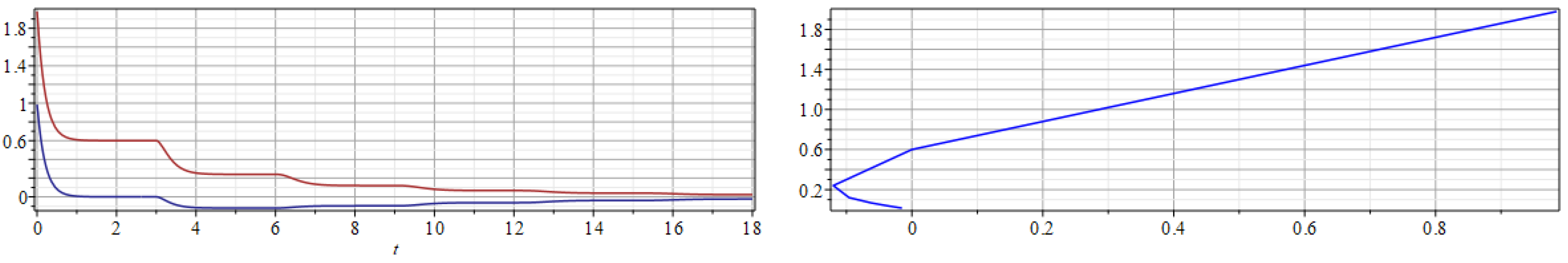
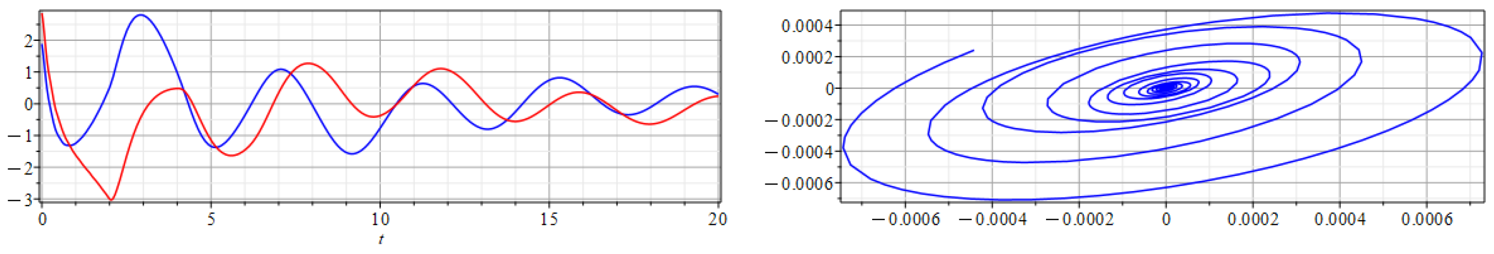
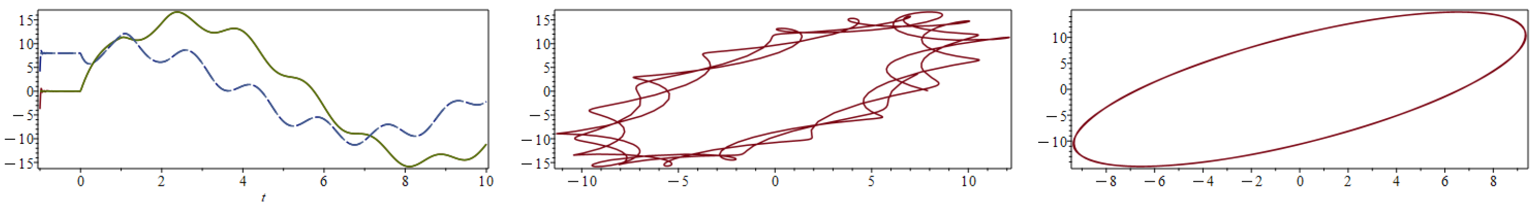
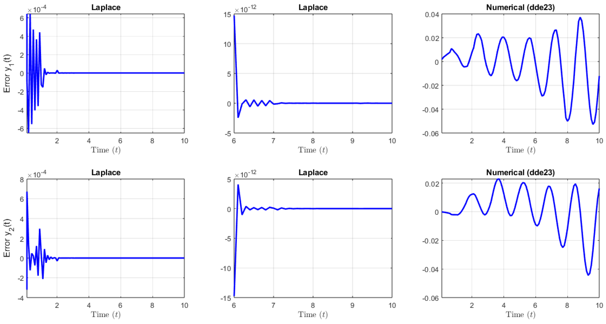
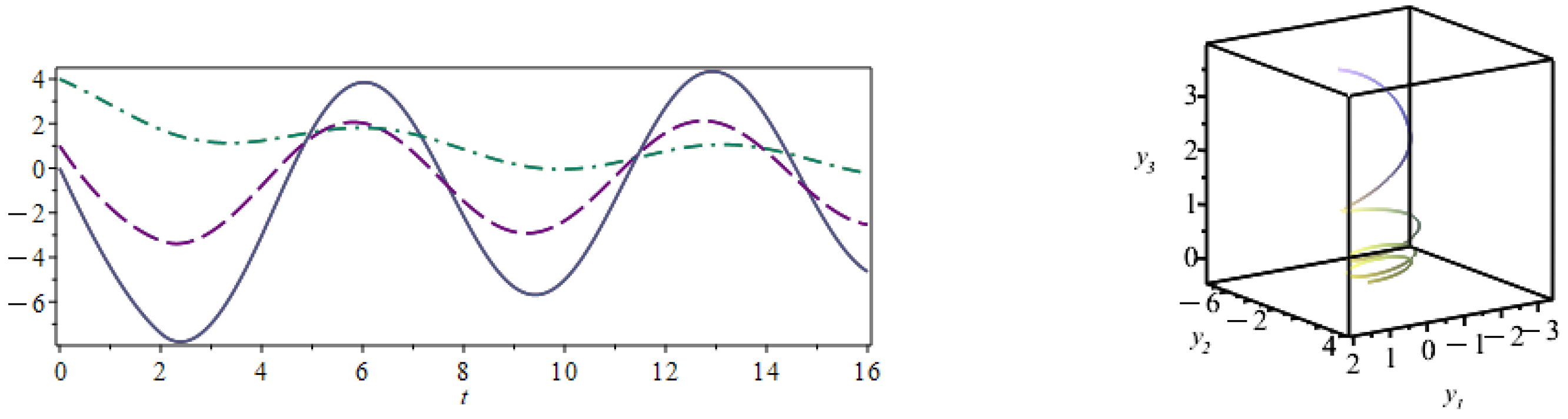
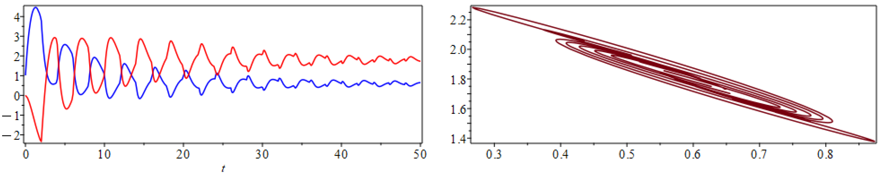
Figure 8 depicts the exact solution given by the MoS and the LT solution. We also include the graphs of the LT solution in the phase space for different time intervals. The solution approaches a limit cycle (an ellipse), but certainly not in an obvious way. Observe that in Figure 8 (plot in the middle), where the t-range has passed well beyond that of the MoS solution, that there is still no compelling evidence to suggest that the solution will eventually stabilize. As a matter of fact the behavior of the solution seems chaotic. This is because the first term in the sum decays very slowly and therefore continues to perturb the limit cycle until around $t=500$, after which $\left|2\left[\mathfrak{Re}{\displaystyle \sum _{k=1}^{\infty }}{c}_{j,k}{e}^{r_{j,k}t}\right]\right|<1.0\times {10}^{-6}$.

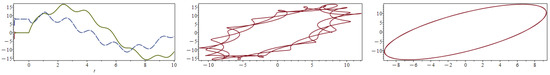
Figure 8. Solution of the linear system of RDDEs (27) over $t\in [0,12]$ using both the MoS and the LTM (left). The components of the solution are $y_1\left(t\right)$ (dashed-blue) and $y_2\left(t\right)$ (solid red). Solution (LT) in the phase space for $t\in [0,36]$ (middle) and for large t (right).

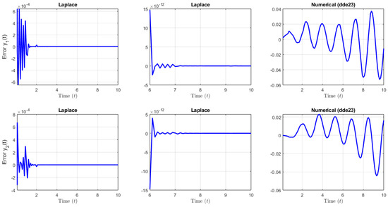
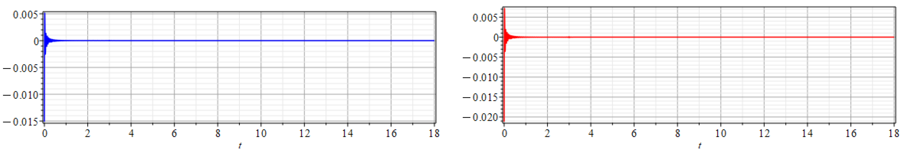
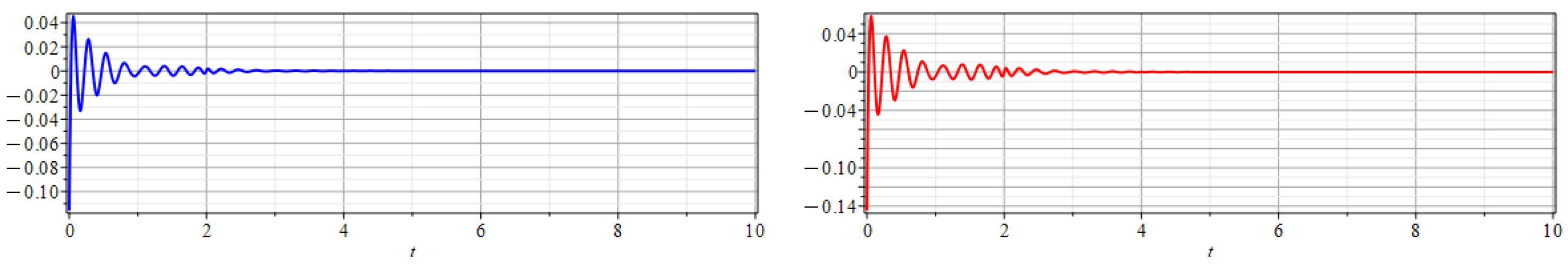
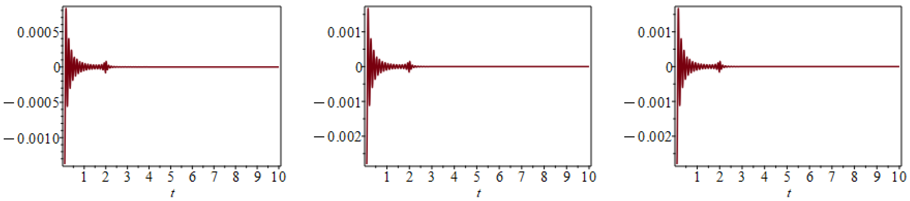
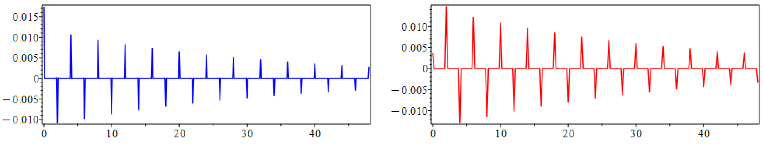
This is a remarkable aspect of some particular linear systems of RDDEs, since this type of dynamic behavior is not achievable for analogous (in this case, first-order $2\times 2$) linear ODE systems. On the left hand-side of Figure 9, we include the graph of the absolute errors of each of the components of the LT solution. The LT solution becomes increasingly more accurate as t increases. For example, the maximum error for $t>6$ is approximately ${10}^{-11}$. On the other hand, on the right-hand side of Figure 9, it can be seen that the error of the numerical solution produced by the dde23 built-in Matlab function increases and that it is much larger than the one generated by the analytical LT solution. Similar results have been found for other types of linear DDEs [32,59]. It is important to remark that the truncated LT solution was produced with only 15 terms, and can be evaluated at any time t.

Figure 9. Errors of the truncated LT solution (15 terms) of the linear system of RDDEs (27) over $t\in [0,10]$ (left-hand side) and over $t\in [6,10]$ (middle). Errors of the numerical solution (dde23) of the linear system of RDDEs (27) over $t\in [0,10]$ (right-hand side).

Example 5.

In this example we present a system in which the matrices A, $B\in {\mathbb{R}}^{3\times 3}$.

$$\begin{array}{cccc}\hfill y^{\prime }\left(t\right)& ={\displaystyle \frac{11}{100}}\left[\begin{array}{ccc}-2& -1& 0\\ -1& -2& 0\\ 1& 0& -2\end{array}\right]y\left(t\right)-{\displaystyle \frac{1}{5}}\left[\begin{array}{ccc}0& 2& 3\\ 0& 4& 5\\ 1& 0& 0\end{array}\right]y(t-2),\hfill & & t>0,\hfill \\ \hfill y\left(t\right)& =H\left(t\right)=\left[\begin{array}{c}1-2t-t^2\\ -2t^2-4t\\ 4+t^2\end{array}\right],\hfill & & t\in [-2,0].\hfill \end{array}$$

(29)

Here, the matrices A and B do not commute. Consequently, we again rely on (18) to obtain the approximates for the locus of the three infinite sequences of poles. These approximates are given by

$$s_{j,k}=\frac{W_k\left(\tau {\lambda }_j\right)}{\tau },j=1..3,k\in \mathbb{N}$$

in which the three eigenvalues of B are $1/5$ and $-1/2$$\pm \sqrt{17}/10$. As is the case with most of our examples, these approximates are sufficiently close to the actual complex poles so that one can compute them all in a single do-loop.

Remark 2.

It is, however, worth emphasizing that from a practical standpoint, one must truncate the LT series solution. In this example, we used $N=15$; hence, the do-loop only computed 45 of the actual poles.

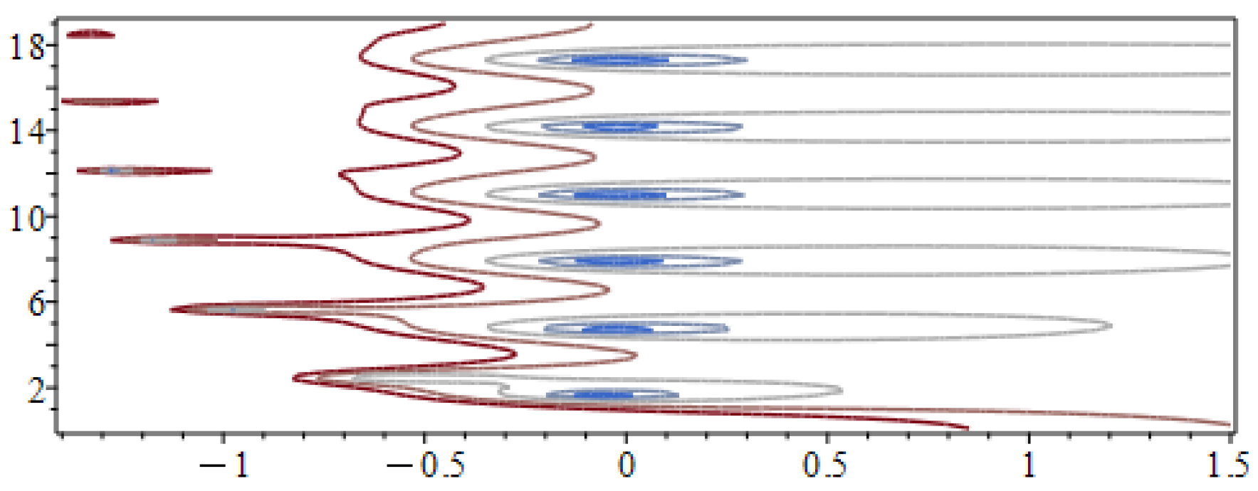
Figure 10 clearly depicts the locus of the three sequences of poles in the complex plane. Figure 11 depicts the exact solution given by the MoS and the LT solution. We also include the graphs of the LT solution in the phase space. In Figure 12, we include the graph of the absolute errors of each of the components of the solution. The LT solution is relatively accurate despite the fact that we only used 15 terms in this example. Notice that the error decreases with time.

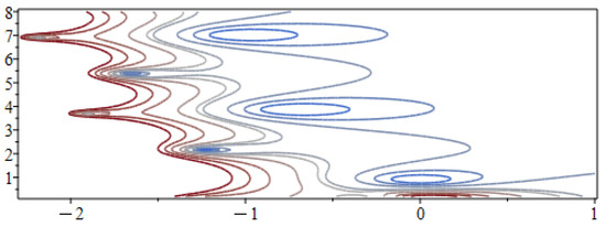
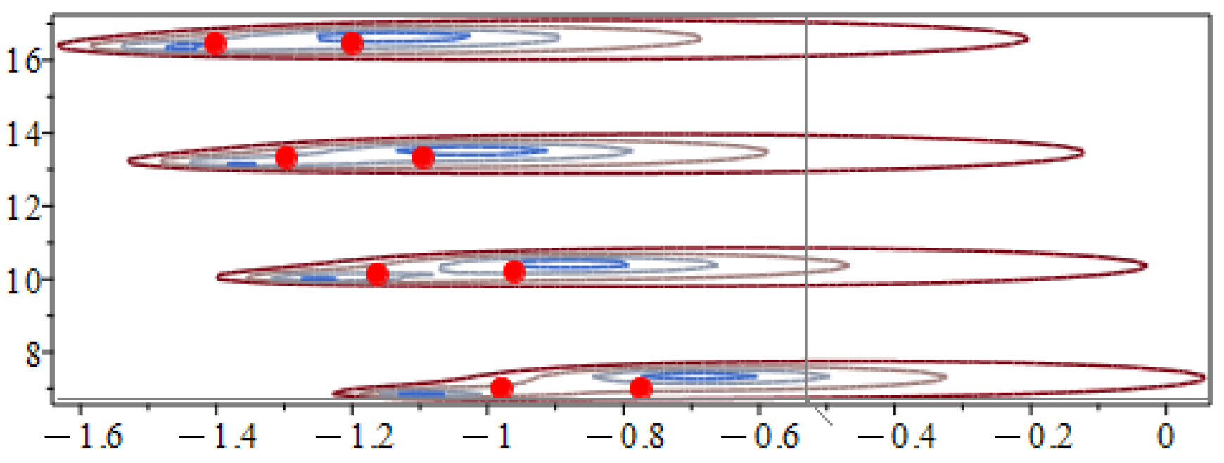
Figure 10. Sequence of poles in the complex plane for the linear system of RDDEs (29).

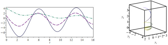
Figure 11. Solution of the linear system of RDDEs (29) over $t\in [0,16]$ using the MoS and the LTM (left). The components of the solution are $y_1\left(t\right)$ (dashed), $y_2\left(t\right)$ (solid) and $y_3\left(t\right)$ (dashed-point). Solution (LT) in the phase space for $t\in [0,25]$ (right).

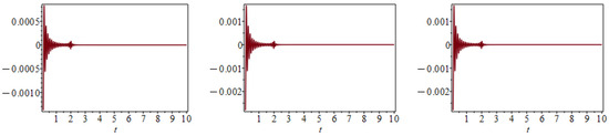
Figure 12. Absolute errors of the solution of the linear system of RDDEs (29) over $t\in [0,10]$ using LTM. For $y_1\left(t\right)$ on the (left), $y_2\left(t\right)$ on the (middle) and $y_3\left(t\right)$ on the (right).

3.2. Linear NDDE Examples

In this subsection, we deal exclusively with examples of systems of first-order linear NDDEs. As mentioned before, oftentimes for the NDDEs, we need to rely on numerical methods to compute the poles or roots of the characteristic equation. The linear systems have the following form $y^{\prime }\left(t\right)=Ay\left(t\right)+By(t-\tau )+C{y}^{\prime }(t-\tau )$.

Example 6.

Consider this first linear system of NDDEs:

$$\begin{array}{cccc}\hfill y^{\prime }\left(t\right)& =-\frac{1}{6}\left[\begin{array}{cc}5& 1\\ 2& 8/3\end{array}\right]y\left(t\right)+\frac{1}{3}\left[\begin{array}{cc}1& 1\\ 2& 1\end{array}\right]y(t-\tau )+\frac{2}{9}\left[\begin{array}{cc}-3& 1\\ 4& -1\end{array}\right]y^{\prime }(t-\tau ),\hfill & & t>0,\hfill \\ \hfill y\left(t\right)& =H\left(t\right)=\left[\begin{array}{c}{(\tau /2-t)}^2\\ -(\tau +t)t\end{array}\right],\hfill & & t\in [-\tau ,0].\hfill \end{array}$$

(30)

where $\tau =2$. In this example, the matrices in (30) do not satisfy the condition $CA+B=0$. Hence, the required complex poles must be computed numerically. Recall, that for a NDDE the approximate placements of these poles for $\left|s\right|$ large and $\mathfrak{Im}\left(s\right)>0$ are given by (12). Therefore, substituting the eigenvalues of C into (12) provides one with the sequences of initial guesses

$$s_{1,k}=\frac{ln(-4/9+2\sqrt{5}/9)+2k\pi i}{\tau },s_{2,k}=\frac{ln(-4/9-2\sqrt{5}/9)+2k\pi i}{\tau },k\in \mathbb{N}.$$

(31)

Remark 3.

The eigenvalue ${\lambda }_2=$$-4/9$$-2\sqrt{5}/9$ is negative. When this is the case, it is advisable, for some softwares, to use the equivalent initial guess $s_{2,k}=\frac{ln\left(\left|{\lambda }_2\right|\right)+(2k-1)\pi i}{\tau }$.

All of the complex poles have negative real parts, and there are three real poles: two with negative real parts ($s=r_{-1},r_{-2}$,) and the other at exactly $s=r=0$. Therefore, the solution assumes the form

$$y_j\left(t\right)=a_{j,0}+a_{j,1}{e}^{r_{-1}t}+a_{j,2}{e}^{r_{-2}t}+2\left[\mathfrak{Re}\sum _{k=1}^{\infty }{c}_{j,k}{e}^{r_{j,k}t}\right]j=1,2,$$

(32)

with the coefficients being given by (22). Hence, the solution approaches a stable equilibrium point at $(a_{1,0},a_{2,0})=(46/77,138/77)$ as $t\to \infty .$

Figure 13 depicts the location of the sequence of poles in the complex plane. Notice that there are two clear sequences of poles. Figure 14 depicts the solution given by the LT solution. It includes the plot in the phase space. The solution approaches a stable equilibrium point. In Figure 15, we include the graph of the absolute errors. The LT solution is relatively accurate despite the fact that we only used 50 terms. Notice that the error decreases with time.

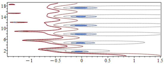
Figure 13. Sequence of poles in the complex plane for the linear system of NDDEs (30).

Figure 14. Solution of the linear system of NDDEs (30) over $t\in [0,50]$ using the LTM (left). The components of the solution are $y_1\left(t\right)$ (blue) and $y_2\left(t\right)$ (red). Solution in the phase space for $t\in [30,50]$ (right).

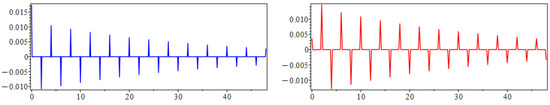
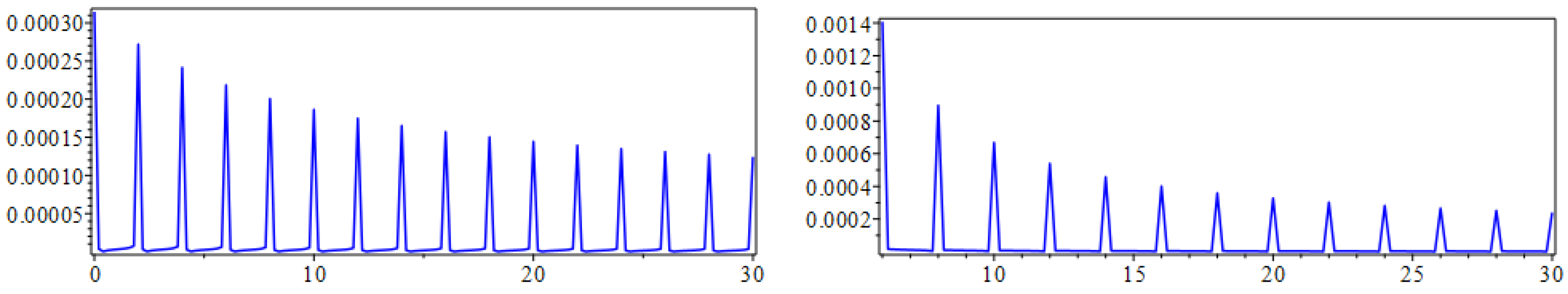
Figure 15. Absolute errors of the solution of the linear system of NDDEs (30) over $t\in [0,50]$ using LTM. For $y_1\left(t\right)$ on the (left) and $y_2\left(t\right)$ on the (right).

Example 7.

Consider the following linear system of NDDEs:

$$\begin{array}{cc}\hfill y^{\prime }\left(t\right)=& \left[\begin{array}{cc}\frac{1}{24}+\frac{ln\left(\frac{29}{30}\right)}{6}& -\frac{1}{40}+\frac{ln\left(\frac{29}{30}\right)}{2}\\ -\frac{1}{72}+\frac{5ln\left(\frac{29}{30}\right)}{18}& \frac{1}{120}+\frac{5ln\left(\frac{29}{30}\right)}{6}\end{array}\right]y\left(t\right)+\left[\begin{array}{cc}-\frac{1}{24}-\frac{ln\left(\frac{29}{30}\right)}{6}& \frac{1}{40}-\frac{ln\left(\frac{29}{30}\right)}{2}\\ \frac{1}{72}-\frac{5ln\left(\frac{29}{30}\right)}{18}& -\frac{1}{120}-\frac{5ln\left(\frac{29}{30}\right)}{6}\end{array}\right]y(t-2)\hfill \\ \hfill & +\left[\begin{array}{cc}1& 0\\ 0& 1\end{array}\right]y^{\prime }(t-2),t>0,\hfill \\ \hfill & y\left(t\right)=H\left(t\right)=\left[\begin{array}{c}5-{(t+1)}^{2}sin\left(3\pi t\right)-\frac{1}{5}(t^2-1)-\frac{2}{5}{\left(\frac{29}{30}\right)}^t\\ \\ -\frac{5}{3}+\frac{1}{3}{(t+1)}^{2}sin\left(3\pi t\right)-\frac{1}{3}(t^2-1)-\frac{2}{3}{\left(\frac{29}{30}\right)}^t\end{array}\right],t\in [-2,0].\hfill \end{array}$$

(33)

In this final example, we present a system where the solution asymptotically approaches a limit cycle. The matrices in this NDDE satisfy the condition $CA+B=0.$ Recall, from Section 2, that this enables one to acquire exact expressions for all of the poles, using the factorization

$$D=sI-A-(B+Cs)e^{-s\tau }=(sI-A)(I-C{e}^{-s\tau }).$$

(34)

From which, it follows that

$$det\left(D\right)=(s-1/20)(s-ln(29/30)){(1-e^{-s\tau })}^2.$$

(35)

The complex poles (for $\mathfrak{Im}\left(r_k\right)>0$) are determined by the ${(1-e^{-s\tau })}^2$ factor, and are therefore given by

$$r_{j,k}=\frac{ln\left({\lambda }_j\right)+2k\pi i}{\tau }=\frac{2k\pi i}{\tau }j,k\in \mathbb{N}.$$

(36)

Remark 4.

The matrix C has a repeated eigenvalue, $\lambda =1$ (with multiplicity 2). And there are four real poles, at $r=1/20,r=ln(29/30)$ and $r=0$ (with multiplicity 2). Dealing with an infinite sequence of complex poles of order 2 typically requires one to incorporate the appropriate modifications, when applying the Cauchy residue theorem to compute the ILT [36]. Fortunately, it is not necessary to do so for this particular system. Observe that the matrix D can be (further) factored as

$$D=(1-e^{-s\tau })(sI-A).$$

(37)

And as a result, both of the numerators (determinants) in (9) include a common factor of $1-e^{-s\tau }$. It can also be shown, however, that there is an additional common factor of $(s-1/20)$. Therefore, when simplified, one finds that

$$Y_j=\frac{det\left(N_j\right)}{det\left(D\right)}=\frac{(1-e^{-s\tau })(s-1/20)R_j\left(s\right)}{(s-1/20)(s-ln(29/30)){(1-e^{-s\tau })}^2},$$

(38)

where $R_j\left(s\right)$ denotes the remaining terms, once the common factors are removed, and where $R_j(ln(29/30))\ne 0.$ From which, it is now evident that what we have is a removable singularity at $r=1/20$, two real poles, both of order one, at $r_{-1}=ln(29/30)$ and $r_0=0,$ along with an infinite sequence of order one complex poles (above the real axis) at $r_{j,k}=\frac{2k\pi i}{\tau }$.

Therefore, the solution assumes the form

$$y_j\left(t\right)=a_{j,0}+a_{j,1}{\left(\frac{29}{30}\right)}^t+2\left[\mathfrak{Re}\sum _{k=1}^{\infty }{c}_{j,k}{e}^{\frac{2k\pi i}{\tau }t}\right]j=1,2,$$

(39)

with the coefficients being given by (37). For example, $c_{j,k}=\frac{1}{2}\frac{R_j\left(\frac{2k\pi i}{\tau }\right)}{(\frac{2k\pi i}{\tau }-ln(29/30))}$.

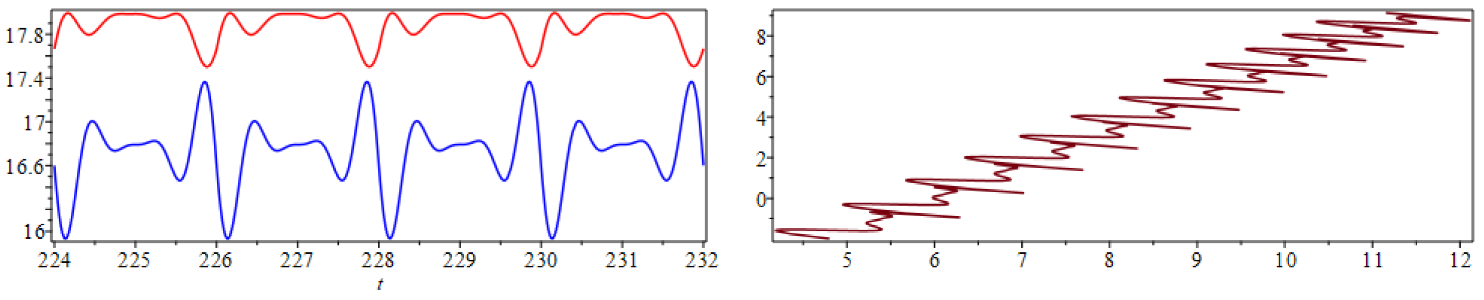
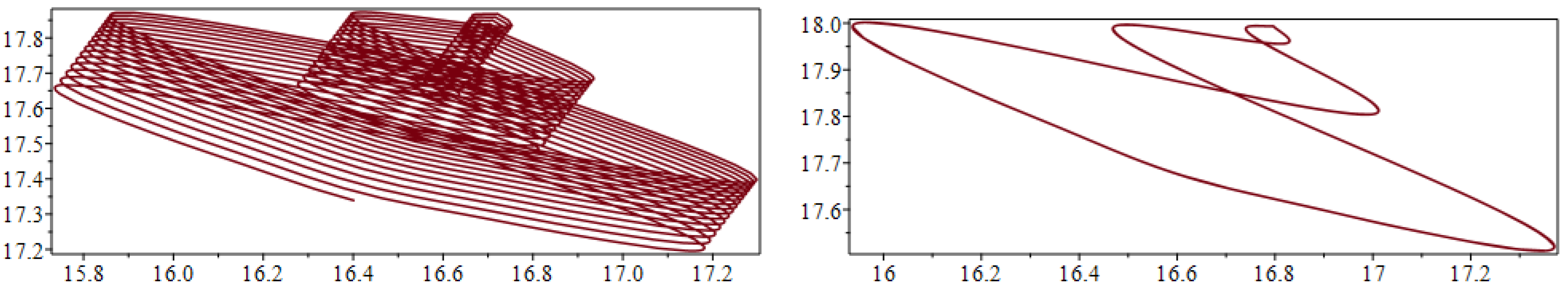
Notice, by virtue of the fact that all of the complex poles have zero real part, that the series component of the solution is a regular harmonic Fourier series. Hence, as $t\to \infty ,$ both $y_1\left(t\right)$ and $y_2\left(t\right)$ oscillate steadily with a frequency of $\tau =2$. This can be seen clearly on the left-hand side of Figure 16 where the solution given by the LT solution is displayed. Figure 16 and Figure 17 also include plots in the phase space. Observe that on the right-hand side of Figure 16 where the t-range is small, but has surpassed that of the MoS solution, there is scant evidence to suggest that the solution will eventually stabilize. However, it appears that for $t=120$ to 150, the LT solution eventually stabilizes to the limit cycle, as observed on the right-hand side of Figure 17. In Figure 18, we include the graph of the relative errors. The LT solution is relatively accurate despite the fact that we only used 50 terms. In this particular example the error does not asymptotically approach zero but it has a lower bound. This bound appears due to the fact that the functions $y_1\left(t\right)$ and $y_2\left(t\right)$ asymptotically approach a periodic steady state. The correct LT solution must therefore do likewise, which explains why the sum in (39) is a regular Fourier series. As a consequence, as $t\to \infty$, the truncated LT solution exhibits the same type behavior as, e.g., the regular Fourier cosine series for a saw tooth function, where the absolute error is also periodic, with spikes at each of the endpoints. Note that the errors can be reduced by increasing the number of terms in the series.

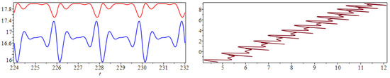
Figure 16. Solution of the linear system of NDDEs (33) over $t\in [224,232]$ using the LTM (left). The components of the solution are $y_1\left(t\right)$ (blue) and $y_2\left(t\right)$ (red). Solution in the phase space for $t\in [0,24]$ (right).

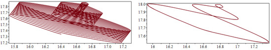
Figure 17. Solution of the linear system of NDDEs (33) in the phase space for $t\in [120,150]$ (left) and $t\in [329,339]$ (right).

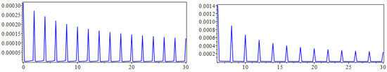
Figure 18. Relative errors of the solution of the linear system of NDDEs (33) over $t\in [0,30]$ using LTM. For $y_1\left(t\right)$ on the (left) and $y_2\left(t\right)$ on the (right).

4. Conclusions

In this work, we developed and implemented a new approach for obtaining analytical solutions of systems of linear RDDEs and NDDEs. The proposed analytical approach is based on the LT, ILT and Cauchy’s residue theorem. We discovered that there are a variety of situations that can arise depending on the spectral properties of the matrices and whether the system involves an RDDE or NDDE. For RDDEs the method for finding the poles is dictated by the commutative property of the matrices A and B. The obtained solutions have the particular form of an infinite non-harmonic Fourier series. One of the main advantages of the proposed approach is the closed-form of the solutions, which are accurate and easy to evaluate at any time. In addition, it allows one to study the asymptotic behavior of the solutions. Thus, the proposed approach provides a practical solution for the user community. Another remarkable result is that for some linear systems of both retarded and neutral delay differential equations, the location of the poles, can lead to solutions which approach asymptotically to a limit cycle. This is an interesting aspect since this type of dynamic behavior is not achievable for autonomous systems of linear ODEs. We provided several examples illustrating the methodology. The examples were designed to facilitate a discussion on how the spectral properties of the matrices determine and affect the procedure for computing the solution. These examples show the variability and richness of the behavior of the solutions of DDEs. Finally, we made comparisons between the LTM and the MoS solutions in order to show the reliability of the proposed approach, even when the truncated series is limited to only a handful of terms. Future works or open problems are related to dealing with repeated poles and discontinuous input functions in linear systems of DDEs. This would require careful attention when applying the ILT and the use of the Cauchy residue theorem.

References

- Deb, A.; Roychoudhury, S.; Sarkar, G. Analysis and Identification of Time-Invariant Systems, Time-Varying Systems, and Multi-Delay Systems Using Orthogonal Hybrid Functions: Theory and Algorithms with MATLAB®; Springer: Berlin/Heidelberg, Germany, 2016; Volume 46. [Google Scholar]
- Aljahdaly, N.H.; El-Tantawy, S. On the multistage differential transformation method for analyzing damping Duffing oscillator and its applications to plasma physics. Mathematics 2021, 9, 432. [Google Scholar] [CrossRef]
- Alfifi, H.Y. Feedback control for a diffusive and delayed Brusselator model: Semi-analytical solutions. Symmetry 2021, 13, 725. [Google Scholar] [CrossRef]
- Arino, J.; Van Den Driessche, P. Time delays in epidemic models. In Delay Differential Equations and Applications; Springer: Dordrecht, The Netherlands, 2006; pp. 539–578. [Google Scholar]
- Ebaid, A.; Al-Enazi, A.; Albalawi, B.Z.; Aljoufi, M.D. Accurate approximate solution of Ambartsumian delay differential equation via decomposition method. Math. Comput. Appl. 2019, 24, 7. [Google Scholar] [CrossRef]
- Halanay, A.; Safta, C.A. A critical case for stability of equilibria of delay differential equations and the study of a model for an electrohydraulic servomechanism. Syst. Control Lett. 2020, 142, 104722. [Google Scholar] [CrossRef]
- Nelson, P.W.; Murray, J.D.; Perelson, A.S. A model of HIV-1 pathogenesis that includes an intracellular delay. Math. Biosci. 2000, 163, 201–215. [Google Scholar] [CrossRef] [PubMed]
- Ruschel, S.; Pereira, T.; Yanchuk, S.; Young, L.S. An SIQ delay differential equations model for disease control via isolation. J. Math. Biol. 2019, 79, 249–279. [Google Scholar] [CrossRef] [PubMed]
- Smith, H.L. An Introduction to Delay Differential Equations with Applications to the Life Sciences; Springer: New York, NY, USA, 2011; Volume 57. [Google Scholar]
- van den Berg, R.; Lefeber, E.; Rooda, K. Modeling and control of a manufacturing flow line using partial differential equations. IEEE Trans. Control. Syst. Technol. 2007, 16, 130–136. [Google Scholar] [CrossRef]
- Diekmann, O.; Van Gils, S.A.; Verduyn Lunel, S.M.; Walther, H.O. Delay Equations: Functional-, Complex-, and Nonlinear Analysis; Springer Science & Business Media: Berlin/Heidelberg, Germany, 2012; Volume 110. [Google Scholar]
- Bellen, A.; Guglielmi, N.; Ruehli, A.E. Methods for linear systems of circuit delay differential equations of neutral type. IEEE Trans. Circuits Syst. Fundam. Theory Appl. 1999, 46, 212–215. [Google Scholar] [CrossRef]
- Ospanov, A. Delay Differential Equations and Their Application to Micro Electro Mechanical Systems. Master’s Thesis, VCU University, Richmond, VA, USA, 2018. [Google Scholar]
- Bellour, A.; Bousselsal, M.; Laib, H. Numerical Solution of Second-Order Linear Delay Differential and Integro-Differential Equations by Using Taylor Collocation Method. Int. J. Comput. Methods 2020, 17, 1950070. [Google Scholar] [CrossRef]
- Chamekh, M.; Elzaki, T.M.; Brik, N. Semi-analytical solution for some proportional delay differential equations. SN Appl. Sci. 2019, 1, 148. [Google Scholar] [CrossRef]
- Cimen, E.; Uncu, S. On the solution of the delay differential equation via Laplace transform. Commun. Math. Appl. 2020, 11, 379–387. [Google Scholar]
- Eftekhari, S.A. A differential quadrature procedure with regularization of the Dirac-delta function for numerical solution of moving load problem. Lat. Am. J. Solids Struct. 2015, 12, 1241–1265. [Google Scholar] [CrossRef]
- Jaaffar, N.T.; Abdul Majid, Z.; Senu, N. Numerical Approach for Solving Delay Differential Equations with Boundary Conditions. Mathematics 2020, 8, 1073. [Google Scholar] [CrossRef]
- Jamilla, C.; Mendoza, R.; Mező, I. Solutions of neutral delay differential equations using a generalized Lambert W function. Appl. Math. Comput. 2020, 382, 125334. [Google Scholar] [CrossRef]
- Jamilla, C.U.; Mendoza, R.G.; Mendoza, V.M.P. Explicit solution of a Lotka-Sharpe-McKendrick system involving neutral delay differential equations using the r-Lambert W function. Math. Biosci. Eng. 2020, 17, 5686–5708. [Google Scholar] [CrossRef]
- Mayorga, C.J.; Castro, M.Á.; Sirvent, A.; Rodríguez, F. On the Construction of Exact Numerical Schemes for Linear Delay Models. Mathematics 2023, 11, 1836. [Google Scholar] [CrossRef]
- Shampine, L.F.; Thompson, S. Solving ddes in matlab. Appl. Numer. Math. 2001, 37, 441–458. [Google Scholar] [CrossRef]
- Shampine, L.F.; Thompson, S. Numerical solution of delay differential equations. In Delay Differential Equations; Springer: Boston, MA, USA, 2009; pp. 1–27. [Google Scholar]
- Cimen, E.; Ekinci, Y. Numerical method for a neutral delay differential problem. Int. J. Math. Comput. Sci. 2017, 1, 1–11. [Google Scholar]
- Izadi, M.; Yüzbaşı, Ş.; Adel, W. A new Chelyshkov matrix method to solve linear and nonlinear fractional delay differential equations with error analysis. Math. Sci. 2023, 17, 267–284. [Google Scholar] [CrossRef]
- Aziz, N.H.A.; Laham, M.F.; Majid, Z.A. Numerical Approaches of Block Multistep Method for Propagation of Derivatives Discontinuities in Neutral Delay Differential Equations. Alex. Eng. J. 2023, 75, 577–588. [Google Scholar] [CrossRef]
- Arnal, A.; Casas, F.; Chiralt, C. Magnus integrators for linear and quasilinear delay differential equations. J. Comput. Appl. Math. 2023, 431, 115273. [Google Scholar] [CrossRef]
- Bauer, R.J.; Mo, G.; Krzyzanski, W. Solving delay differential equations in S-ADAPT by method of steps. Comput. Methods Programs Biomed. 2013, 111, 715–734. [Google Scholar] [CrossRef] [PubMed]
- Kalmár-Nagy, T. Stability analysis of delay-differential equations by the method of steps and inverse Laplace transform. Differ. Equ. Dyn. Syst. 2009, 17, 185–200. [Google Scholar] [CrossRef]
- Kaslik, E.; Sivasundaram, S. Analytical and numerical methods for the stability analysis of linear fractional delay differential equations. J. Comput. Appl. Math. 2012, 236, 4027–4041. [Google Scholar] [CrossRef]
- Heffernan, J.M.; Corless, R.M. Solving some delay differential equations with computer algebra. Math. Sci. 2006, 31, 21–34. [Google Scholar]
- Kerr, G.; González-Parra, G. Accuracy of the Laplace transform method for linear neutral delay differential equations. Math. Comput. Simul. 2022, 197, 308–326. [Google Scholar] [CrossRef]
- Bellen, A.; Guglielmi, N.; Zennaro, M. Numerical stability of nonlinear delay differential equations of neutral type. J. Comput. Appl. Math. 2000, 125, 251–263. [Google Scholar] [CrossRef]
- Enright, W.; Hayashi, H. Convergence analysis of the solution of retarded and neutral delay differential equations by continuous numerical methods. SIAM J. Numer. Anal. 1998, 35, 572–585. [Google Scholar] [CrossRef]
- Diwaker; Chakraborty, A. Exact solution of time-dependent Schrodinger equation for two state problem in Laplace domain. Chem. Phys. Lett. 2015, 638, 133–136. [Google Scholar] [CrossRef]
- Sherman, M.; Kerr, G.; González-Parra, G. Analytic solutions of linear neutral and non-neutral delay differential equations using the Laplace transform method: Featuring higher order poles and resonance. J. Eng. Math. 2023, 140, 12. [Google Scholar] [CrossRef]
- Sayyari, Y.; Dehghanian, M.; Park, C. Some stabilities of system of differential equations using Laplace transform. J. Appl. Math. Comput. 2023, 69, 3113–3129. [Google Scholar] [CrossRef]
- Asl, F.M.; Ulsoy, A.G. Analysis of a system of linear delay differential equations. J. Dyn. Syst. Meas. Control 2003, 125, 215–223. [Google Scholar] [CrossRef]
- Castro, M.Á.; García, M.A.; Martín, J.A.; Rodríguez, F. Exact and nonstandard finite difference schemes for coupled linear delay differential systems. Mathematics 2019, 7, 1038. [Google Scholar] [CrossRef]
- Castro, M.Á.; Sirvent, A.; Rodríguez, F. Nonstandard finite difference schemes for general linear delay differential systems. Math. Methods Appl. Sci. 2021, 44, 3985–3999. [Google Scholar] [CrossRef]
- Yi, S.; Ulsoy, A.G.; Nelson, P.W. Solution of systems of linear delay differential equations via Laplace transformation. In Proceedings of the 45th IEEE Conference on Decision and Control, San Diego, CA, USA, 13–15 December 2006; IEEE: Piscataway, NJ, USA, 2006; pp. 2535–2540. [Google Scholar]
- Vyasarayani, C. Galerkin approximations for neutral delay differential equations. J. Comput. Nonlinear Dyn. 2013, 8, 021014. [Google Scholar] [CrossRef]
- Zafer, N. Discussion: “Analysis of a System of Linear Delay Differential Equations” (Asl, F.M., and Ulsoy, A.G., 2003, ASME J. Dyn. Syst., Meas., Control, 125, pp. 215–223). J. Dyn. Syst. Meas. Control. 2007, 129, 121–122. [Google Scholar] [CrossRef]
- Elshenhab, A.M.; Wang, X.T. Representation of solutions of linear differential systems with pure delay and multiple delays with linear parts given by non-permutable matrices. Appl. Math. Comput. 2021, 410, 126443. [Google Scholar] [CrossRef]
- Medved’, M.; Pospíšil, M. Representation of solutions of systems of linear differential equations with multiple delays and linear parts given by nonpermutable matrices. J. Math. Sci. 2018, 228, 276–289. [Google Scholar] [CrossRef]
- Pospíšil, M. Representation and stability of solutions of systems of functional differential equations with multiple delays. Electron. J. Qual. Theory Differ. Equ. 2012, 2012, 1–30. [Google Scholar] [CrossRef]
- Pospíšil, M. Representation of solutions of systems of linear differential equations with multiple delays and nonpermutable variable coefficients. Math. Model. Anal. 2020, 25, 303–322. [Google Scholar] [CrossRef]
- Brown, J.W.; Churchill, R.V. Fourier Series and Boundary Value Problems; McGraw-Hill Book Company: New York, NY, USA, 2009. [Google Scholar]
- Conway, J.B. Functions of One Complex Variable II; Springer Science & Business Media: Berlin/Heidelberg, Germany, 2012; Volume 159. [Google Scholar]
- Sedletskii, A.M. On the summability and convergence of non-harmonic Fourier series. Izv. Math. 2000, 64, 583. [Google Scholar] [CrossRef]
- Young, R.M. An Introduction to Non-Harmonic Fourier Series, Revised Edition, 93; Elsevier: Amsterdam, The Netherlands, 2001. [Google Scholar]
- Russell, D.L. Nonharmonic Fourier series in the control theory of distributed parameter systems. J. Math. Anal. Appl. 1967, 18, 542–560. [Google Scholar] [CrossRef]
- Hale, J.K.; Verduyn Lunel, S.M. Introduction to Functional Differential Equations; Springer Science & Business Media: Berlin/Heidelberg, Germany, 2013; Volume 99. [Google Scholar]
- Kerr, G.; González-Parra, G.; Sherman, M. A new method based on the Laplace transform and Fourier series for solving linear neutral delay differential equations. Appl. Math. Comput. 2022, 420, 126914. [Google Scholar] [CrossRef]
- Brito, P.B.; Fabião, M.F.; St. Aubyn, A.G. The Lambert function on the solution of a delay differential equation. Numer. Funct. Anal. Optim. 2011, 32, 1116–1126. [Google Scholar] [CrossRef]
- Corless, R.M.; Gonnet, G.H.; Hare, D.E.; Jeffrey, D.J.; Knuth, D.E. On the LambertW function. Adv. Comput. Math. 1996, 5, 329–359. [Google Scholar] [CrossRef]
- Lambert, J.H. Observationes variae in mathesin puram. Acta Helv. 1758, 3, 128–168. [Google Scholar]
- Scott, T.C.; Mann, R.; Martinez, R.E. General relativity and quantum mechanics: Towards a generalization of the Lambert W function A Generalization of the Lambert W Function. Appl. Algebra Eng. Commun. Comput. (AAECC) 2006, 17, 41–47. [Google Scholar] [CrossRef]
- Sherman, M.; Kerr, G.; González-Parra, G. Comparison of Symbolic Computations for Solving Linear Delay Differential Equations Using the Laplace Transform Method. Math. Comput. Appl. 2022, 27, 81. [Google Scholar] [CrossRef]
Disclaimer/Publisher’s Note: The statements, opinions and data contained in all publications are solely those of the individual author(s) and contributor(s) and not of MDPI and/or the editor(s). MDPI and/or the editor(s) disclaim responsibility for any injury to people or property resulting from any ideas, methods, instructions or products referred to in the content. |
© 2024 by the authors. Licensee MDPI, Basel, Switzerland. This article is an open access article distributed under the terms and conditions of the Creative Commons Attribution (CC BY) license (https://creativecommons.org/licenses/by/4.0/).