Explicit Integrating Factor Runge–Kutta Method for the Extended Fisher–Kolmogorov Equation

Abstract

The extended Fisher–Kolmogorov (EFK) equation is an important model for phase transitions and bistable phenomena. This paper presents some fast explicit numerical schemes based on the integrating factor Runge–Kutta method and the Fourier spectral method to solve the EFK equation. The discrete global convergence of these new schemes is analyzed rigorously. Three numerical examples are presented to verify the theoretical analysis and the efficiency of the proposed schemes.

1. Introduction

The Fisher–Kolmogorov (FK) equation was first proposed by Fisher [1] and Kolmogorov [2] in 1937 to describe the interaction between the spread and adaptation of biological populations. By adding a stabilizing fourth-order derivative term to the FK equation, Collent [3] and Saarloos [4] proposed the extended FK (EFK) equation, which is a very important mathematical and physical model and has been widely used in many physics and engineering applications. In this paper, we consider the following EFK model with periodic boundary conditions:

$$\left\{\begin{array}{c}\begin{array}{cc}{\partial }_{t}v=-\kappa {\Delta }^{2}v+\Delta v+g\left(v\right),\hfill & \hfill (\mathit{x},t)\in \Omega \times (0,T],\\ v(\mathit{x},0)=v_0\left(\mathit{x}\right),\hfill & \hfill \mathit{x}\in \Omega ,\end{array}\hfill \end{array}\right.$$

(1)

where $\Omega \in {[a,b]}^d,(d=1,2)$ is a bounded area and $\kappa$ is a positive constant. The function $g\left(v\right)=-G^{\prime }\left(v\right)$ and $G\left(v\right)=\frac{1}{4}{(v^2-1)}^2$ is a double-well potential. When $\kappa =0$ in (1), the EFK model reduces to the classical FK model. We assume that the function $g\left(v\right)$ exhibits Lipschitz continuity with respect to $\Omega$, where the Lipschitz constant L is defined as follows

$$\underset{v\in \mathbf{R}}{max}\left|g^{\prime }\left(v\right)\right|\le L.$$

The EFK model (1) can be viewed as an $L^2$ gradient flow associated with the following energy

$$E\left(v\right)={\int }_{\Omega }\left(\frac{\kappa }{2}{|\Delta v|}^2+\frac{1}{2}{|\nabla v|}^2+G\left(v\right)\right)dx,$$

which is diminishing in time, i.e., $\frac{d}{dt}E\left(v\right)\le 0$.

All the above properties are determined by the inherent nature of the physical model. Thus, in order to avoid non-physical effects in the simulations over a long period of time, it is highly desirable to design a structure-preserving numerical scheme. There have been some excellent results in numerical research on the EFK model, such as the spline configuration method [5], nonlinear/linear finite difference schemes [6], and the local boundary integral method [7]. However, these works do not consider the physical properties of the EFK model. Recently, Sun et al. [8,9] proposed two convex splitting variable step BDF2/BDF3 schemes for the EFK model, and the proposed schemes preserve the modified discrete energy dissipation law.

The development of high-precision numerical schemes for PDEs of gradient-flow-type has attracted much attention. In this direction, it is worth mentioning the integrating factor Runge–Kutta (IFRK) method [10]. The IFRK method has demonstrated remarkable advantages for equations with stiff linear terms. The exponential function in this method provides the exact solution of the linear part, so the stiffness does not restrict the step size and the solution to the nonlinear part may be approximated explicitly. As a result, the IFRK method is often explicit [11,12]. In recent years, the IFRK method has attracted widespread attention for solving partial differential equations. Ju et al. [13] proposed the MBP-preserving IFRK method for semilinear parabolic equations. Li et al. [14] proposed a class of unconditional MBP-preserving IFRK schemes for the conservative Allen–Cahn equation. Zhang et al. [15,16] developed a class of high-order structure-preserving IFRK methods for the Allen–Cahn equation. Then, they further [17] proposed and analyzed a series of temporal up to fourth-order unconditionally structure-preserving single-step methods to solve the Allen–Cahn equation, and introduced parametric IFRK (pIFRK) schemes which can be used to construct higher-order parametric single-step methods. To the authors’ best knowledge, there are very few works in the literature on high-precision numerical methods for the EFK model. The objective of this paper is to develop a class of efficient, high-order-accurate schemes for the EFK model based on the explicit IFRK method coupled with non-decreasing abscissas (eIFRK+) [13,18].

The rest of the article is arranged as follows: In Section 2, a class of eIFRK+ schemes is proposed for solving the EFK model, and the corresponding theoretical analysis is given in Section 3. Numerical experiments are presented to test the performance of the proposed numerical schemes in Section 4, and some concluding remarks are given in Section 5.

2. eIFRK+ Fourier-Spectral Schemes for EFK Model

Define a periodic spatial grid ${\cap }_h=\left\{(x_i,y_j)=\left(a+ih,a+jh\right),0\le i,j\le N-1)\right\}$ with $h=\frac{b-a}{N}$ (N is even). All of the 2D periodic grid functions defined on ${\cap }_h$ are denoted by ${\mathcal{M}}_h$.

The discrete Fourier transform $\tilde{\varphi }=Q\varphi$ and the corresponding inverse transform $\varphi =Q^{-1}\tilde{\varphi }$ are defined by [19]

$$\begin{array}{cc}\hfill {\tilde{\varphi }}_{pq}& =\frac{h^2}{{(b-a)}^2}{\displaystyle \sum _{i=0}^{N-1}}{\displaystyle \sum _{j=0}^{N-1}}{\varphi }_{ij}exp\left(-\mathrm{i}\frac{2p\pi (x_i-a)}{b-a}-\mathrm{i}\frac{2q\pi (y_j-a)}{b-a}\right),\hfill \\ \hfill & p,q=0,\pm 1,\pm 2,\cdots ,\frac{N}{2},\hfill \end{array}$$

(2)

$$\begin{array}{cc}\hfill {\varphi }_{ij}& ={\displaystyle \sum _{p=-N/2}^{N/2}}{\displaystyle \sum _{q=-N/2}^{N/2}}{\tilde{\varphi }}_{pq}\left(t\right)exp\left(\mathrm{i}\frac{2p\pi (x_i-a)}{b-a}+\mathrm{i}\frac{2q\pi (y_j-a)}{b-a}\right),\hfill \\ \hfill & {\tilde{\varphi }}_{-\frac{N}{2},q}={\tilde{\varphi }}_{\frac{N}{2},q},{\tilde{\varphi }}_{p,-\frac{N}{2}}={\tilde{\varphi }}_{p,\frac{N}{2}},\hfill \end{array}$$

(3)

respectively. We further define the operators ${\widehat{D}}_x$ and ${\widehat{D}}_y$ on $\widehat{{\mathcal{M}}_h}=\left\{Q\varphi \right|\varphi \in {\mathcal{M}}_h\}$ as

$${\left({\widehat{D}}_x\tilde{\varphi }\right)}_{pq}=\frac{2p\pi \mathrm{i}}{b-a}{\tilde{\varphi }}_{pq},{\left({\widehat{D}}_y\tilde{\varphi }\right)}_{pq}=\frac{2q\pi \mathrm{i}}{b-a}{\tilde{\varphi }}_{pq},$$

and then, the Laplace operator can be approximated by

$${\Delta }_N=Q^{-1}({\widehat{D}}_x^2+{\widehat{D}}_y^2)Q.$$

Next, we give some fully discrete eIFRK+ schemes for solving the EFK equation. Let $\tau =\frac{T}{M}$ and define the time node as $t_k=k\tau$ ($k=0,1,\cdots M$). According to the definitions of discrete spatial operators presented in Section 2, the EFK model (1) is reduced to the following nonlinear ordinary differential equations (ODEs) in time

$$\frac{d}{dt}v\left(t\right)={\mathcal{L}}_{N}v\left(t\right)+g\left(v\left(t\right)\right),$$

(4)

where ${\mathcal{L}}_N=-\kappa {\Delta }_N^2+{\Delta }_N$ and $v\left(t\right)=\left\{v_{ij}\left(t\right)\right\}\in {\mathcal{M}}_h$. Let $v\left(t\right)=e^{t{\mathcal{L}}_N}u\left(t\right)$, then Equation (4) can be transformed into

$$\frac{d}{dt}u\left(t\right)=e^{-t{\mathcal{L}}_N}g\left(e^{t{\mathcal{L}}_N}u\left(t\right)\right),$$

(5)

which can be solved by the following s-stage classical RK scheme [18]

$$\left\{\begin{array}{c}{u}^{\left(0\right)}=u^k,\hfill \\ u^{\left(i\right)}={\displaystyle {\displaystyle \sum _{j=0}^{i-1}}}[{\eta }_{ij}{u}^{\left(j\right)}+\tau {\gamma }_{ij}{e}^{-t_k^{\left(j\right)}{\mathcal{L}}_N}g\left(e^{t_k^{\left(j\right)}{\mathcal{L}}_N}{u}^{\left(j\right)}\right)],1\le i\le n,\hfill \\ u^{k+1}=u^{\left(n\right)},\hfill \end{array}\right.$$

(6)

where $t_k^{\left(j\right)}=t_k+d_j\tau$, $d_j$ is the abscissa at each j-th layer. ${\eta }_{ij}\ge 0$ and ${\displaystyle \sum _{j=0}^{i-1}}{\eta }_{ij}=1$, ${\gamma }_{ij}$ is a real constant.

Since $v^{\left(j\right)}=e^{t_k^{\left(j\right)}{\mathcal{L}}_{{}_N}}{u}^{\left(j\right)}$, then (6) becomes

$$\left\{\begin{array}{c}{v}^{\left(0\right)}=v^k,\hfill \\ v^{\left(i\right)}={\displaystyle {\displaystyle \sum _{j=0}^{i-1}}}{e}^{(d_i-d_j)\tau {\mathcal{L}}_{{}_N}}[{\eta }_{ij}{v}^{\left(j\right)}+\tau {\gamma }_{ij}g\left(v^{\left(j\right)}\right)],1\le i\le n,\hfill \\ v^{k+1}=v^{\left(n\right)},\hfill \end{array}\right.$$

(7)

where $d_i-d_j\ge 0$, $d_0=0$ and $d_n=1$. By a simple derivation, the above scheme can be rewritten in the following equivalent form [13]:

$$\left\{\begin{array}{c}{v}^{\left(0\right)}=v^k,\hfill \\ v^{\left(i\right)}=e^{d_i\tau {\mathcal{L}}_N}{v}^k+\tau {\displaystyle {\displaystyle \sum _{j=0}^{i-1}}}{\epsilon }_{ij}{e}^{(d_i-d_j)\tau {\mathcal{L}}_N}g\left(v^{\left(j\right)}\right),1\le i\le n,\hfill \\ v^{k+1}=v^{\left(n\right)},\hfill \end{array}\right.$$

(8)

where ${\displaystyle {\displaystyle \sum _{j=0}^{i-1}}}{\epsilon }_{ij}\le 1$, ${\gamma }_{ij}={\epsilon }_{ij}-{\displaystyle {\displaystyle \sum _{s=j+1}^{i-1}}}{\eta }_{is}{\epsilon }_{sj}$.

Some specific cases of system (7) are presented, which are denoted by eIFRK+$(n,q)$, where q denotes the time accuracy:

$$\mathbf{eIFRK}+(\mathbf{1},\mathbf{1}):v^{k+1}=e^{\tau {\mathcal{L}}_N}[v^k+\tau g\left(v^k\right)].$$

(9)

$$\mathbf{eIFRK}+(\mathbf{2},\mathbf{2}):\left\{\begin{array}{c}{v}^{\left(1\right)}=e^{\tau {\mathcal{L}}_N}[v^k+\tau g\left(v^k\right)],\hfill \\ v^{k+1}=\frac{1}{2}{e}^{\tau {\mathcal{L}}_N}{v}^k+\frac{1}{2}[v^{\left(1\right)}+\tau g\left(v^{\left(1\right)}\right)].\hfill \end{array}\right.$$

(10)

$$\mathbf{eIFRK}+(\mathbf{3},\mathbf{3}):\left\{\begin{array}{c}{v}^{\left(1\right)}=\frac{1}{2}{e}^{\frac{2\tau }{3}{\mathcal{L}}_N}{v}^k+\frac{1}{2}{e}^{\frac{2\tau }{3}{\mathcal{L}}_N}[v^k+\frac{4\tau }{3}g\left(v^k\right)],\hfill \\ v^{\left(2\right)}=\frac{2}{3}{e}^{\frac{2\tau }{3}{\mathcal{L}}_N}{v}^k+\frac{1}{3}[v^{\left(1\right)}+\frac{4\tau }{3}g\left(v^{\left(1\right)}\right)],\hfill \\ v^{k+1}=\frac{59}{128}{e}^{\tau {\mathcal{L}}_N}{v}^k+\frac{15}{128}{e}^{\tau {\mathcal{L}}_N}[v^k+\frac{4\tau }{3}g\left(v^k\right)]+\frac{27}{64}{e}^{\frac{\tau }{3}{\mathcal{L}}_N}[v^{\left(2\right)}+\frac{4\tau }{3}g\left(v^{\left(2\right)}\right)].\hfill \end{array}\right.$$

(11)

$$\mathbf{eIFRK}+(\mathbf{4},\mathbf{4}):\left\{\begin{array}{c}{v}^{\left(1\right)}={\mathrm{e}}^{\frac{\tau }{2}{\mathcal{L}}_N}[v^k+\frac{\tau }{2}g\left(v^k\right)],\hfill \\ v^{\left(2\right)}=\frac{1}{2}{e}^{\frac{\tau }{2}{\mathcal{L}}_N}[v^k-\frac{\tau }{2}g\left(v^k\right)]+\frac{1}{2}[v^{\left(1\right)}+\tau g\left(v^{\left(1\right)}\right)],\hfill \\ v^{\left(3\right)}=\frac{1}{9}{e}^{\tau {\mathcal{L}}_N}[v^k-\tau g\left(v^k\right)]+\frac{2}{9}{e}^{\frac{\tau }{2}{\mathcal{L}}_N}[v^{\left(1\right)}-\frac{3\tau }{2}g\left(v^{\left(1\right)}\right)]\hfill \\ +\frac{2}{3}{e}^{\frac{\tau }{2}{\mathcal{L}}_N}[v^{\left(2\right)}+\frac{3\tau }{2}g\left(v^{\left(2\right)}\right)],\hfill \\ v^{k+1}=\frac{1}{3}{e}^{\frac{\tau }{2}{\mathcal{L}}_N}[v^{\left(1\right)}+\frac{\tau }{2}g\left(v^{\left(1\right)}\right)]+\frac{1}{3}{e}^{\frac{\tau }{2}{\mathcal{L}}_N}{v}^{\left(2\right)}+\frac{1}{3}[v^{\left(3\right)}+\frac{\tau }{2}g\left(v^{\left(3\right)}\right)].\hfill \end{array}\right.$$

(12)

3. Discrete Error Estimate

In this section, the discrete error estimation of the scheme (8) is discussed. We first give one lemma that helps to prove the discrete error estimation for the scheme.

Lemma 1 

([20]). If a matrix A is negative semi-definite, then we have $\parallel e^{tA}{\parallel }_2\le 1$ for $t>0$, where ${\parallel ·\parallel }_2$ denotes the standard vector or matrix $L^2$-norm.

Theorem 1. 

(Error estimate.) Assume that $v_0\in H_{per}^p(\Omega )$=$\{v\in H_{per}^p(\Omega )andvs.is\Omega -periodic\}$ with $p>4$ and the solution to the EFK model belongs to ${\mathcal{C}}^{q+1}(0,T;H_{per}^p(\Omega ))$. Under the conditions of Lemma 1, then the numerical solutions $\left\{{\mathit{V}}^k\right\}\in {\mathcal{M}}_h$ generated by the eIFRK+ schemes (8) with ${\mathit{V}}^0=I_h{v}_0$ satisfy the following error estimate

$$\parallel {\mathit{V}}^k-I_{h}v\left(t_k\right){\parallel }_2\le \tilde{c}\left(h^p+{\tau }^q\right).$$

(13)

where $\tilde{c}$ is a positive constant depending on τ and h. $I_h$: $H_{per}^p(\Omega )\to {\mathcal{M}}_h$ is a sample operator as $I_h\left(v(x,y)\right)=\left\{v(x_i,y_j)\right\}$.

Proof. 

Let $\mathit{Z}\left(t\right)=\mathit{V}\left(t\right)-I_{h}v(x,y,t)$ with $\mathit{Z}\left(0\right)=0$; the difference between Equations (1) and (4) leads to

$$\begin{array}{cc}\hfill & {\displaystyle \frac{d}{dt}}\mathit{Z}\left(t\right)={\mathcal{L}}_N\mathit{Z}\left(t\right)+g\left(\mathit{V}\left(t\right)\right)-g\left(I_h\left(v\right)\right)+R_N\left(v\right),\hfill \end{array}$$

(14)

where the truncated error $R_N\left(v\right)=\mathcal{L}\left(I_{h}v\right)-{\mathcal{L}}_N\left(I_{h}v\right)$ satisfies $\parallel R_N\parallel {}_2\le c{h}^p$.

Multiplying both sides of (14) by $e^{-t{\mathcal{L}}_N}$, then we have

$$\frac{d}{dt}\left(e^{-t{\mathcal{L}}_N}\mathit{Z}\left(t\right)\right)=e^{-t{\mathcal{L}}_N}\left(g\left(\mathit{V}\left(t\right)\right)-g\left(I_h\left(v\right)\right)+R_N\left(v\right)\right).$$

(15)

Using the eIFRK+ scheme (8), we have the following fully discrete scheme for the above equation

$$\left\{\begin{array}{c}{\mathit{Z}}^{\left(i\right)}=e^{d_i\tau {\mathcal{L}}_N}{\mathit{Z}}^k+\tau {\displaystyle {\displaystyle \sum _{j=0}^{i-1}}}{\epsilon }_{ij}{e}^{(d_i-d_j)\tau {\mathcal{L}}_N}\left(g\left({\mathit{V}}^{\mathit{j}}\right)-g\left(I_h{v}^{\left(j\right)}\right)+R_N\left(v^{\left(j\right)}\right)\right),1\le i\le n-1,\hfill \\ {\mathit{Z}}^{k+1}=e^{\tau {\mathcal{L}}_N}{\mathit{Z}}^k+\tau {\displaystyle {\displaystyle \sum _{i=0}^{n-1}}}{\rho }_i{e}^{(1-d_i)\tau {\mathcal{L}}_N}\left(g\left({\mathit{V}}^{\mathit{j}}\right)-g\left(I_h{v}^{\left(j\right)}\right)+R_N\left(v^{\left(j\right)}\right)\right)+{\xi }^k,\hfill \end{array}\right.$$

(16)

where ${\displaystyle {\displaystyle \sum _{j=0}^{i-1}}}{\epsilon }_{ij}\le 1$, ${\displaystyle {\displaystyle \sum _{i=0}^{n-1}}}{\epsilon }_{ni}={\displaystyle {\displaystyle \sum _{i=0}^{n-1}}}{\rho }_i=1$, ${\xi }^k$ is the truncation error satisfying $\parallel {\xi }^k{\parallel }_2\le c^{\prime }{\tau }^{q+1}$.

By the Lipschitz condition for $g\left(v\right)$, we have

$$\parallel g\left({\mathit{V}}^{\mathit{j}}\right)-g\left(I_h{v}^{\left(j\right)}\right){\parallel }_2\le L\parallel {\mathit{V}}^{\mathit{j}}-I_h{v}^{\left(j\right)}{\parallel }_2=L{\parallel {\mathit{Z}}^{\left(j\right)}\parallel }_2.$$

Combination of the above estimates leads to

$$\begin{array}{cc}\hfill \parallel Z^{\left(i\right)}{\parallel }_2& \le \parallel e^{d_i\tau {\mathcal{L}}_N}{Z}^k{\parallel }_2+\tau \parallel {\displaystyle \sum _{j=0}^{i-1}}{\epsilon }_{ij}{e}^{(d_i-d_j)\tau {\mathcal{L}}_N}(g\left({\mathit{V}}^{\mathit{j}}\right)-g\left(I_h{v}^{\left(j\right)}\right)){\parallel }_2\hfill \\ \hfill & +\tau \parallel {\displaystyle \sum _{j=0}^{i-1}}{\epsilon }_{ij}{e}^{(d_i-d_j)\tau {\mathcal{L}}_N}{R}_N\left(v^{\left(j\right)}\right){\parallel }_2\hfill \\ \hfill & \le \parallel Z^k{\parallel }_2+L\tau {\displaystyle \sum _{j=0}^{i-1}}{\parallel Z^{\left(j\right)}\parallel }_2+c{h}^p\tau .\hfill \end{array}$$

By using the Gronwall’s inequality, we further have

$$\begin{array}{cc}\hfill \parallel {\mathit{Z}}^{\left(i\right)}{\parallel }_2& \le e^{L(i+1)\tau }(\parallel {\mathit{Z}}^k{\parallel }_2+c{h}^p\tau ).\hfill \end{array}$$

(17)

Similar to the estimation of $\parallel {\mathit{Z}}^{k+1}{\parallel }_2$, we have

$$\begin{array}{cc}\hfill \parallel {\mathit{Z}}^{k+1}{\parallel }_2& \le \parallel {\mathit{Z}}^k{\parallel }_2+L\tau {\displaystyle \sum _{i=0}^{n-1}}{\parallel {\mathit{Z}}^{\left(i\right)}\parallel }_2+c{h}^p\tau +\parallel {\xi }^k{\parallel }_2.\hfill \end{array}$$

(18)

Combining (17) with (18), we have

$$\begin{array}{cc}\hfill \parallel {\mathit{Z}}^{k+1}{\parallel }_2& \le \parallel {\mathit{Z}}^k{\parallel }_2+L\tau {\displaystyle \sum _{i=0}^{n-1}}{e}^{L(i+1)\tau }({\parallel {\mathit{Z}}^k\parallel }_2+c{h}^p\tau )+c{h}^p\tau +\parallel {\xi }^k{\parallel }_2\hfill \\ \hfill & \le \parallel {\mathit{Z}}^k{\parallel }_2+L\tau n{e}^{Ln\tau }\parallel {\mathit{Z}}^k{\parallel }_2+c^{\prime \prime }{h}^p\tau +c^{\prime }{\tau }^{q+1}.\hfill \end{array}$$

(19)

Summing the above inequality from $k=0$ to m and using Gronwall’s inequality, we obtain the desired result

$$\parallel {\mathit{Z}}^{m+1}\parallel {|}_2\le e^{LnT{e}^{LT}}(c^{\prime \prime }{h}^{p}T+c^{\prime }{\tau }^{q}T)\le \tilde{c}(h^p+{\tau }^q).$$

□

4. Numerical Experiments

We examine the accuracy and efficiency of the proposed method through three numerical experiments, including convergence and diminishing energy.

Example 1. 

The purpose of the first numerical experiment is to verify the role of parameter κ. Consider the 1D EFK model in $\Omega =[-4,4]$ with the initial condition

$$v_0\left(x\right)=-sin\left(\pi x\right).$$

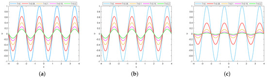
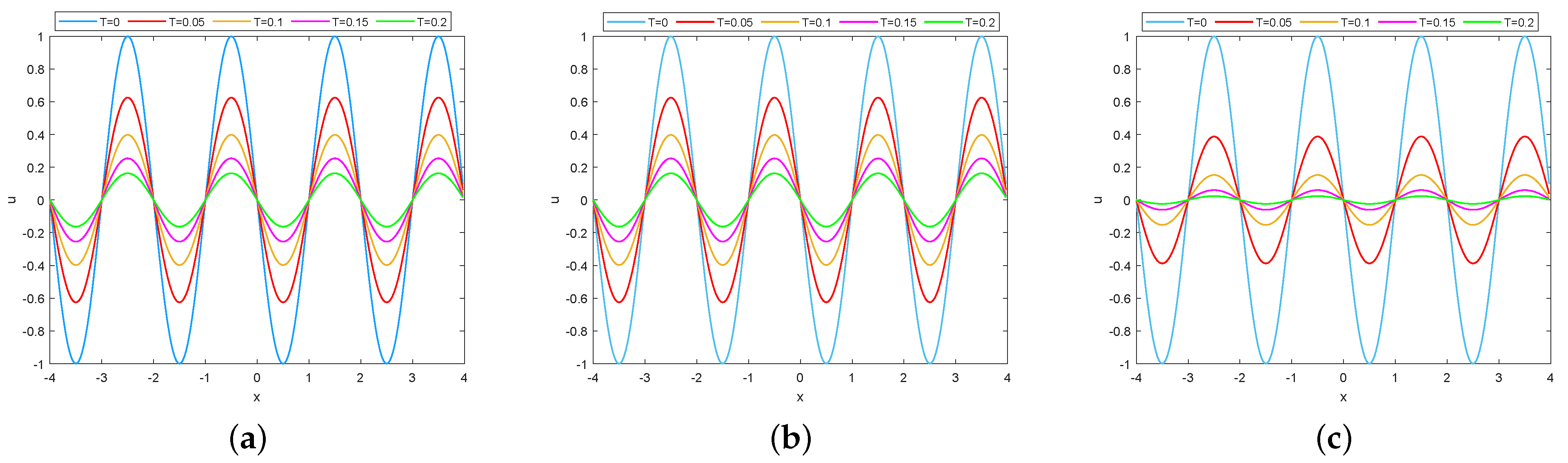
We choose $N=256$ and $\tau =0.01$. Figure 1 shows the numerical results using scheme eIFRK+(4,4) at different times $t=0,0.05,0.1,0.15,0.2$. It is observed that the dynamic evolution of $\kappa =0$ is almost identical to that of $\kappa ={10}^{-4}$. However, when $\kappa =0.1$, the solution rapidly evolves from the initial state to zeros, which illustrates that the coefficient κ in the EFK model is a stable parameter.

Figure 1. Numerical solutions with different $\kappa$ values for Example 1. (a) $\kappa =0$; (b) $\kappa ={10}^{-4}$; (c) $\kappa =0.1$.

Example 2. 

To show the temporal accuracy and convergence of the proposed schemes, we consider the 2D EFK model in $\Omega =[-16,16{]}^2$ with $\kappa =0.01$ and the initial condition

$$\begin{array}{cc}\hfill v_0(x,y)& =0.1-0.2cos\left(\frac{\pi (x-12)}{16}\right)sin\left(\frac{\pi (y-12)}{16}\right)\hfill \\ \hfill & +0.1{cos}^2\left(\frac{\pi (x+10)}{32}\right){sin}^2\left(\frac{\pi (y+3)}{32}\right)-0.2{sin}^2\left(\frac{\pi x}{8}\right)cos\left(\frac{\pi (y-6)}{8}\right).\hfill \end{array}$$

We adopt the uniform $1024\times 1024$ spatial mesh, which is sufficiently fine so that the errors caused by the spatial approximation can be ignored. The error between two different time steps τ and $\frac{\tau }{2}$ is calculated. The computational results are presented in Table 1. One may see that the numerical orders of time accuracy are close to the optimal order.

Table 1. Temporal errors and convergence orders at $T=1$ with $\kappa =0.01$ and $N=1024$ for Example 2.

eIFRK+	M	Errmax	Rate	Err${}_{{\mathit{L}}^2}$	Rate
$(1,1)$	16	$3.9212\times {10}^{-3}$	-	1.9491$\times {10}^{-2}$	-
	32	$1.9980\times {10}^{-3}$	0.9728	9.8542	0.9840
	64	$1.0086\times {10}^{-3}$	0.9862	4.9540$\times {10}^{-3}$	0.9921
	128	$5.0671\times {10}^{-4}$	0.9931	$2.4837\times {10}^{-3}$	0.9961
$(2,2)$	16	$1.2908\times {10}^{-4}$	-	$6.5886\times {10}^{-4}$	-
	32	$3.3107\times {10}^{-5}$	1.9630	$1.6909\times {10}^{-4}$	1.9622
	64	$8.3832\times {10}^{-6}$	1.9816	$4.2826\times {10}^{-5}$	1.9812
	128	$2.1092\times {10}^{-6}$	1.9908	$1.0776\times {10}^{-5}$	1.9906
$(3,3)$	16	$1.4809\times {10}^{-6}$	-	$5.0559\times {10}^{-6}$	-
	32	$1.8992\times {10}^{-7}$	2.9631	$6.5053\times {10}^{-7}$	2.9583
	64	$2.4046\times {10}^{-8}$	2.9815	$8.2502\times {10}^{-8}$	2.9791
	128	$3.0251\times {10}^{-9}$	2.9907	$1.0388\times {10}^{-8}$	2.9896
$(4,4)$	16	$3.1132\times {10}^{-8}$	-	$1.6382\times {10}^{-7}$	-
	32	$1.9696\times {10}^{-9}$	3.9824	$1.0359\times {10}^{-8}$	3.9830
	64	$1.2395\times {10}^{-10}$	3.9901	$6.5125\times {10}^{-10}$	3.9915
	128	$7.7799\times {10}^{-12}$	3.9939	$4.0823\times {10}^{-11}$	3.9958

Example 3. 

Consider the EFK model in $\Omega =[-1,1{]}^2$ with the initial condition

$$v_0(x,y)=-1+\tanh \left(\frac{0.4-\sqrt{x^2+y^2}}{\epsilon \sqrt{2}}\right)-tanh\left(\frac{0.3-\sqrt{x^2+y^2}}{\epsilon \sqrt{2}}\right).$$

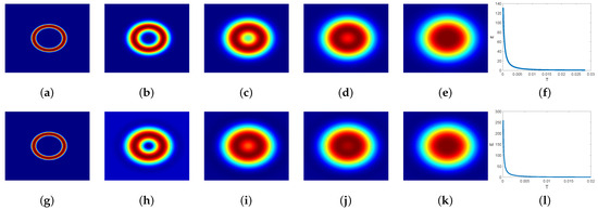
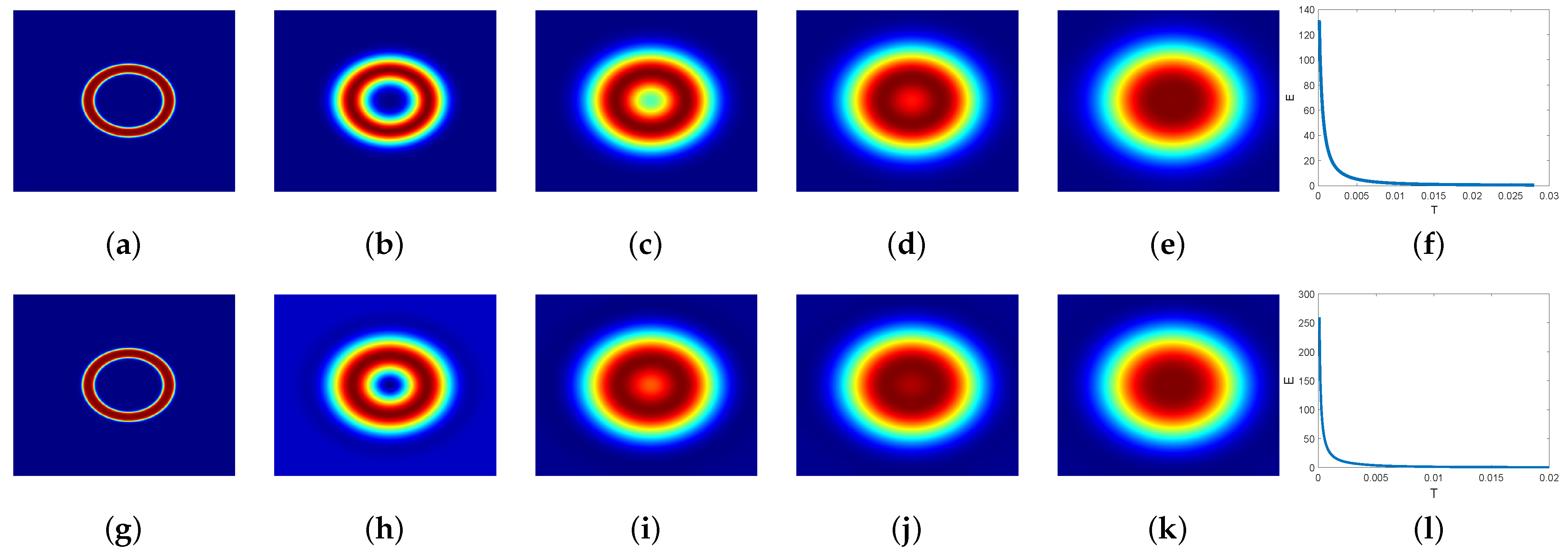
We choose $\epsilon =\frac{5h}{\sqrt{2}tan{h}^{-1}\left(0.9\right)}$, $N=256$, $\tau =0.01$ and different κ, Figure 2 shows the evolutions of the snapshots and the energies of the numerical solutions obtained by the eIFRK+(4,4) scheme. It can be seen that the evolution speed of the numerical solution is largely clipped with the increase in κ, and the energy obtained from the energy image gradually reaches a steady state with decreasing time.

Figure 2. The numerical solution u at different times for Example 3. Top: $\kappa ={10}^{-4}$. Bottom: $\kappa =0.004$. (a) $T=0$; (b) $T=0.004$; (c) $T=0.012$; (d) $T=0.02$; (e) $T=0.028$; (f) $E\left(v\right)$; (g) $T=0$; (h) $T=0.004$; (i) $T=0.012$; (j) $T=0.016$; (k) $T=0.02$; (l) $E\left(v\right)$.

5. Conclusions

Based on the explicit IFRK method coupled with nondecreasing abscissas, we have obtained a class of fast and effective numerical schemes for the EFK model. The optimal error estimates of the fully discrete schemes have been analyzed. Three numerical experiments were carried out to test the accuracy and applicability of the proposed schemes.

References

- Fisher, R.A. The wave of advance of advantageous genes. Ann. Eugen. 1937, 7, 355–369. [Google Scholar] [CrossRef]
- Kolmogorov, A.N.; Petrovskii, I.G.; Piskunov, N.S. A study of the diffusion equation with increase in the quantity of matter, and its application to a biological problem. Mosc. Univ. Math. Bull. 1937, 1, 1–25. [Google Scholar]
- Coullet, P.; Elphick, C.; Repaux, D. Nature of spatial chaos. Phys. Rev. Lett. 1987, 58, 431. [Google Scholar] [CrossRef]
- Saarloos, W.V. Dynamical velocity selection: Marginal stability. Phys. Rev. Lett. 1987, 58, 2571. [Google Scholar] [CrossRef]
- Danumjaya, P.; Pani, A.K. Orthogonal cubic spline collocation method for the extended Fisher–Kolmogorov equation. J. Comput. Appl. Math. 2005, 174, 101–117. [Google Scholar] [CrossRef]
- Li, S.G.; Xu, D.; Zhang, J.; Sun, C.J. A new three-level fourth-order compact finite difference scheme for the extended Fisher–Kolmogorov equation. Appl. Numer. Math. 2022, 178, 41–51. [Google Scholar] [CrossRef]
- Ilati, M.; Dehghan, M. Direct local boundary integral equation method for numerical solution of extended Fisher–Kolmogorov equation. Eng. Comput. 2018, 34, 203–213. [Google Scholar] [CrossRef]
- Sun, Q.H.; Ji, B.Q.; Zhang, L. A convex splitting BDF2 method with variable time-steps for the extended Fisher–Kolmogorov equation. Comput. Math. Appl. 2022, 114, 73–82. [Google Scholar] [CrossRef]
- Sun, Q.H.; Wang, J.D.; Zhang, L.M. A new third-order energy stable technique and error estimate for the extended Fisher–Kolmogorov equation. Comput. Math. Appl. 2023, 142, 198–207. [Google Scholar] [CrossRef]
- Isherwood, L.; Grant, Z.J.; Gottlieb, S. Strong stability preserving integrating factor Runge–Kutta methods. SIAM J. Numer. Anal. 2018, 58, 3276–3307. [Google Scholar] [CrossRef]
- Zhai, S.Y.; Weng, Z.F.; Yang, Y.F. A high order operator splitting method based on spectral deferred correction for the nonlocal viscous Cahn–Hilliard equation. J. Comput. Phys. 2021, 446, 110632. [Google Scholar] [CrossRef]
- Zhai, S.Y.; Weng, Z.F.; Feng, X.L.; He, Y.N. Stability and error estimate of the operator splitting method for the phase field crystal equation. J. Sci. Comput. 2021, 86, 8. [Google Scholar] [CrossRef]
- Ju, L.L.; Li, X.; Qiao, Z.H.; Yang, J. Maximum bound principle preserving integrating factor Runge–Kutta methods for semilinear parabolic equations. J. Comput. Phys. 2021, 439, 110405. [Google Scholar] [CrossRef]
- Li, J.W.; Li, X.; Ju, L.L.; Feng, X.L. Stabilized integrating factor Runge–Kutta method and unconditional preservation of maximum bound principle. SIAM J. Sci. Comput. 2021, 43, A1780–A1802. [Google Scholar] [CrossRef]
- Zhang, H.; Yan, J.Y.; Qian, X.; Chen, X.W.; Song, S.H. Explicit third-order unconditionally structure-preserving schemes for conservative Allen–Cahn equations. J. Sci. Comput. 2022, 90, 1–29. [Google Scholar] [CrossRef]
- Zhang, H.; Yan, J.Y.; Qian, X.; Song, S.H. Numerical analysis and applications of explicit high order maximum principle preserving integrating factor Runge–Kutta schemes for Allen–Cahn equation. Appl. Numer. Math. 2021, 161, 372–390. [Google Scholar] [CrossRef]
- Zhang, H.; Yan, J.Y.; Qian, X.; Song, S.H. Up to fourth-order unconditionally structure-preserving parametric single-step methods for semilinear parabolic equations. Comput. Methods Appl. Mech. Eng. 2022, 393, 114817. [Google Scholar] [CrossRef]
- Shu, C.W.; Osher, S. Efficient implementation of essentially non-oscillatory shock-capturing schemes. J. Comput. Phys. 1988, 77, 439–471. [Google Scholar] [CrossRef]
- Shen, J.; Tang, T.; Wang, L.L. Spectral Methods: Algorithms, Analysis and Applications; Springer Science: London, UK; New York, NY, USA, 2011; Volume 41, pp. 1–45. [Google Scholar]
- Nan, C.X.; Song, H.L. The high-order maximum-principle-preserving integrating factor Runge–Kutta methods for nonlocal Allen–Cahn equation. J. Comput. Phys. 2022, 456, 111028. [Google Scholar] [CrossRef]
Disclaimer/Publisher’s Note: The statements, opinions and data contained in all publications are solely those of the individual author(s) and contributor(s) and not of MDPI and/or the editor(s). MDPI and/or the editor(s) disclaim responsibility for any injury to people or property resulting from any ideas, methods, instructions or products referred to in the content. |
© 2023 by the authors. Licensee MDPI, Basel, Switzerland. This article is an open access article distributed under the terms and conditions of the Creative Commons Attribution (CC BY) license (https://creativecommons.org/licenses/by/4.0/).