Prediction Interval for Compound Conway–Maxwell–Poisson Regression Model with Application to Vehicle Insurance Claim Data

Abstract

Regression models in which the response variable has a compound distribution have applications in actuarial science. For example, the aggregate claim amount in a vehicle insurance portfolio can be modeled using a compound Poisson distribution. In this paper, we propose a regression model, wherein the response variable is assumed to have a compound Conway–Maxwell–Poisson (CMP) distribution. This distribution is a parsimonious two-parameter Poisson distribution that accounts for both over- and under-dispersed count data, making it more suitable for application in various fields. A two-part methodology in the framework of a generalized linear model is proposed to estimate the parameters. Additionally, a method to obtain the prediction interval of the response variable is developed. The workings of the proposed methodology are illustrated through simulated data. An application of the compound CMP regression model to real-life vehicle insurance claims data is presented.

1. Introduction

Compound regression models have applications in various research fields, including economics and finance. In economic consumer theory, for example, compound Poisson regression models are often used to examine the factors that account for the expenditures incurred by tourists during their stay at a location. The factors may include length of stay, type of holiday accommodations, age, occupation, socio-economic status of the tourist, etc. See Gómez-Déniz and Pérez-Rodríguez [1]. In actuarial risk theory, the aggregate claim amount incurred by the insurance company against the claims made by the policyholders is modeled using compound models. See Klugman et al. [2] and Bahnemann [3] for a detailed discussion on compound models, their distributional properties and applications in insurance claim modeling. Jørgensen and Paes De Souza [4] applied the compound Poisson regression model to determine the impact on the conditional mean of the aggregate claim amount caused by factors such as age and model of the vehicle, exposure, deductibles, etc., in the context of car insurance. In this paper, we propose a compound regression model using a two-parameter Poisson distribution. On this topic, some mathematical backgrounds are presented below in order to fix the notations. Let

$$S=\sum _{j=1}^N{Y}_j,$$

(1)

denote the random sum, where the distributions of the random variables N and $Y_1,Y_2,\dots ,Y_N$ are assumed to be discrete and continuous, respectively. Moreover, $\left(Y_j\right)$s are assumed to be independent and identically distributed. Therefore, in the sequel, we refer to $Y_j$s as Y. Further, N and Y in general are assumed to be independent. The above-mentioned S is a compound random variable. Suppose $Y_j$ represents the claim amounts on an insurance portfolio, N denotes the number of claims made, then S represents the aggregate claim amount. When N has a Poisson distribution, the distribution of S is known as the compound Poisson distribution. Though the Poisson distribution is often used in constructing compound distributions, it is not suitable for modeling over- or under-dispersed count data. As an alternative to the Poisson distribution, one can use a generalized Poisson distribution (Consul and Jain [5]) to model count data that are either over- or under-dispersed. Recently, Shmueli et al. [6] studied a two-parameter Poisson distribution developed by Conway and Maxwell [7] known as the Conway–Maxwell–Poisson (CMP) distribution. This is a two-parameter flexible generalization of the Poisson distribution that can model both over- and under-dispersed data and has the feature to include the Poisson, geometric and Bernoulli distributions as special cases. A detailed discussion on the properties of this distribution and its applications can be found in Sellers et al. [8]. Also, Sellers and Premeaux [9] contains a detailed review on CMP regression models. In the context of compound distributions, assuming the CMP and binomial distributions for N and Y in Equation (1), a discrete compound CMP-binomial distribution is developed by Saavithri et al. [10].

Considering the Poisson distribution as the counting distribution, compound Poisson regression models are available in the literature. See Frees et al. [11], Andersen and Bonat [12], and Delong et al. [13]. However, its applicability is limited to data with equi-dispersed counts. To allow for flexibility in the compound regression models in terms of accommodating dispersed counts, a counting distribution that can model both over- and under-dispersed data should be considered. This serves as motivation to use the CMP distribution as the counting distribution to build a compound regression model.

The goal of this work is to create a regression model for S using a CMP distribution for N. The present work is novel because of the distribution used for N and its convolution with the distribution of Y. The problem of obtaining prediction intervals for the response variable S is also addressed. The parameters of the compound regression model are estimated using the generalized linear model (GLM) approach in two cases. In the first case, we assume that data on S are available but not on N and Y. We assume data on both N and Y are available in the latter case. For this case, a two-part likelihood-based estimation procedure is developed within the framework of the GLM. A methodology to obtain the prediction interval (PI) for the response variable of the proposed compound regression model is developed.

The rest of the paper is organized as follows: The compound CMP regression model is given in Section 2. In Section 3, the estimation of the parameters of the proposed regression model using the GLM approach is discussed. Section 4 deals with the suggested methodology for obtaining the prediction intervals for the compound CMP regression model. A numerical illustration of the estimation procedure using simulated data and an application to real-life vehicle insurance claims data is presented in Section 5. The conclusion of the paper is given in Section 6.

2. Compound CMP Regression Model

The probability mass function (pmf) of the random variable N having the CMP distribution is given by

$$P(N=n)={\displaystyle \frac{{\lambda }^n}{{(n!)}^{\nu }Z(\lambda ,\nu )}},n=0,1,2,\dots ,\lambda >0,\nu \ge 0,$$

(2)

where $Z(\lambda ,\nu )={\sum }_{j=0}^{\infty }{\lambda }^j/{(j!)}^{\nu }$ is the normalizing constant. Some important remarks on this distribution are given below. The parameters $\lambda$ and $\nu$ are the location and dispersion parameters, respectively. This pmf is not defined for $\lambda \ge 1$ and $\nu =0$. The mean and variance of N are given by $E\left(N\right)=\lambda {\displaystyle \frac{\partial lnZ(\lambda ,\nu )}{\partial \lambda }}$ and $V\left(N\right)=\lambda {\displaystyle \frac{\partial E\left(N\right)}{\partial \lambda }}$, respectively. When $\nu =1$, the CMP distribution reduces to the Poisson distribution. For $\nu >1$, the distribution is under-dispersed, and for $\nu <1$, it is over-dispersed.

Since the location parameter $\lambda$ of the CMP distribution does not represent its mean, a mean reparameterized form of the distribution is used in building the compound regression model. The pmf of N under the mean-reparametrization is given by

$$P(N=n)={\left({\mu }_1+{\displaystyle \frac{e^{\varphi }-1}{2e^{\varphi }}}\right)}^{n{e}^{\varphi }}{\displaystyle \frac{{(n!)}^{-e^{\varphi }}}{Z({\mu }_1,\varphi )}},n=0,1,2,\dots ,{\mu }_1>0,\varphi \in \mathbb{R},$$

(3)

where $Z({\mu }_1,\varphi )={\sum }_{j=0}^{\infty }{\left({\mu }_1+{\displaystyle \frac{e^{\varphi }-1}{2e^{\varphi }}}\right)}^{j{e}^{\varphi }}{\displaystyle \frac{1}{{(j!)}^{e^{\varphi }}}}$ is the normalizing constant. When $\varphi =0,$ the distribution reduces to the Poisson distribution. For $\varphi >0,$ the distribution is under-dispersed, and for $\varphi <0,$ it is over-dispersed. See Ribeiro Jr et al. [14]. Here, ${\mu }_1\approx {\lambda }^{1/\nu }-{\displaystyle \frac{\nu -1}{2\nu }}$ corresponds to the mean of the distribution and $\varphi =ln\left(\nu \right)$. This approximation works reasonably well for $\nu \le 1$ or $\lambda >{10}^{\nu }$. The mean and variance of N are $E\left(N\right)={\mu }_1$ and $V\left(N\right)={\mu }_1{e}^{-\varphi }$, respectively.

Convolutions can be used to obtain the probability density function (pdf) of the random sum S defined in Equation (1). In Equation (1), $N=0$ implies $S=0$. Let $p_0$ denote the probability mass at $S=0$. Since S is not continuous at zero, the pdf of S is represented as a generalized pdf in terms of Dirac delta function as

$$f\left(s\right)=p_0\delta \left(s\right)+\sum _{i=1}^{\infty }{g}_Y^{*i}\left(s\right)P(N=i),s\ge 0,$$

(4)

where $\delta \left(s\right)$ is the Dirac delta function such that ${\int }_0^{\infty }\delta \left(s\right)ds=1.$ Here, $P(N=i)$ denotes the pmf of the CMP distribution defined in Equation (3), and $g_Y^{*i}(.)$ denotes the pdf of the i-fold convolution of Y, whose distribution is assumed to be continuous with support in ${\mathbb{R}}^{+}$. Note that $p_0=P(N=0)=Z{({\mu }_1,\varphi )}^{-1}$. In this paper, the distribution of Y is considered to be a mean reparameterized gamma distribution. Based on Jorgensen [15] (Chapter 3), the pdf of Y is given by

$$g_Y(y;{\mu }_2,\psi )={\displaystyle \frac{1}{\Gamma \left(\psi \right)}}{\left({\displaystyle \frac{\psi }{{\mu }_2}}\right)}^{\psi }{y}^{\psi -1}exp\left(-{\displaystyle \frac{\psi y}{{\mu }_2}}\right),y>0,{\mu }_2>0,\psi >0,$$

(5)

where ${\mu }_2$ denotes the mean of Y, $\psi$ denotes the dispersion parameter and $\Gamma (.)$ denotes the gamma function. This form is taken for mathematical convenience and to accommodate asymmetry in the distribution of Y. For example, in the context of insurance claim modeling, the individual claim amounts are always positive and often right-skewed. Since the gamma distribution is closed under convolution, we obtain

$$g_Y^{*i}\left(y\right)={\displaystyle \frac{1}{\Gamma \left(\psi \right)}}{\left({\displaystyle \frac{\psi }{i{\mu }_2}}\right)}^{\psi }{y}^{\psi -1}exp\left(-{\displaystyle \frac{\psi y}{i{\mu }_2}}\right),y>0,{\mu }_2>0,\psi >0.$$

(6)

Using Equations (3) and (6) in Equation (4), we obtain

$$f\left(s\right)=p_0\delta \left(s\right)+{\displaystyle \frac{s^{\psi -1}{\psi }^{\psi }}{Z({\mu }_1,\varphi ){\mu }_2^{\psi }\Gamma \left(\psi \right)}}\sum _{i=1}^{\infty }{\left({\mu }_1+{\displaystyle \frac{e^{\varphi }-1}{2e^{\varphi }}}\right)}^{i{e}^{\varphi }}{\displaystyle \frac{{(i!)}^{-e^{\varphi }}}{i^{\psi }}}exp\left({\displaystyle \frac{-\psi s}{i{\mu }_2}}\right),s\ge 0.$$

(7)

The pdf of S defined in Equation (7) is called the compound CMP gamma pdf. For the random sum defined in Equation (1), we have

$$\begin{array}{c}\hfill \left\{\begin{array}{c}E\left(S\right)=E\left(N\right)E\left(Y\right),\hfill \\ V\left(S\right)=E\left(N\right)V\left(Y\right)+V\left(N\right){\left[E\left(Y\right)\right]}^2.\hfill \end{array}\right.\end{array}$$

(8)

See, for instance, Bahnemann [3] (Chapter 4). Using Equation (8), the mean and variance of the compound CMP gamma distribution given in Equation (7) are obtained as

$$\left\{\begin{array}{c}E\left(S\right)={\mu }_1{\mu }_2,\hfill \\ V\left(S\right)={\mu }_2^2{\mu }_1[{\psi }^{-1}+e^{-\varphi }].\hfill \end{array}\right.$$

(9)

To build a compound regression model for S, let $X=(\overrightarrow{1},{\overrightarrow{X}}_1,{\overrightarrow{X}}_2,\dots ,{\overrightarrow{X}}_p)$ denote the design matrix where ${\overrightarrow{X}}_i,i=1,2,\dots ,p$ are the column vectors corresponding to the covariates $X_i,i=1,2,\dots ,p$ and $\overrightarrow{1}$ is the vector of $1^{\prime }s$. Following the GLM procedure given in De Jong et al. [16] (Chapter 5), the model is built by regressing S on X using the log-link function. This is because the log-link function guarantees that the expected value of the response variable is positive. Let $\mu$ denote the expected value of S. Then, the compound CMP gamma regression model is given by

$$\mu =exp\left(X\delta \right),$$

(10)

where $\delta ={({\delta }_0,{\delta }_1,\dots ,{\delta }_p)}^{\prime }$ is a $(p+1)\times 1$ vector of regression parameters. In the context of modeling vehicle insurance claims data, S may denote the aggregate claim amount, and the covariates may denote the driver’s age, vehicle type, and so on. In the sequel, the method of estimating the regression parameters using the likelihood approach is discussed.

3. Parameter Estimation

Consider a sample $\overrightarrow{s}={(s_1,s_2,\dots ,s_r)}^{\prime }$ of r observations on S. Let $D(>0)$ positive values in $\overrightarrow{s}$ and $r-D$ zeros exist. Note that D can be assimilated to be random and $D\sim Binomial(r,1-p_0)$, where $p_0=Z{({\mu }_1,\varphi )}^{-1}$. Therefore, the likelihood function L based on $\overrightarrow{s}$ and $D=d$ is

$$\begin{array}{cc}\hfill L& =\left(\genfrac{}{}{0pt}{}{r}{d}\right)p_0^{r-d}{(1-p_0)}^d\prod _{k=1}^{d}f\left(s_k^{+}\right)\hfill \\ \hfill & =\left(\genfrac{}{}{0pt}{}{r}{d}\right){\left({\displaystyle \frac{1}{Z({\mu }_1,\varphi )}}\right)}^{r-d}{\left(1-{\displaystyle \frac{1}{Z({\mu }_1,\varphi )}}\right)}^d\prod _{k=1}^{d}f\left(s_k^{+}\right),\hfill \end{array}$$

(11)

where $f\left(s_k^{+}\right)={\displaystyle \frac{s_k^{\psi -1}{\psi }^{\psi }}{(Z({\mu }_1,\varphi )-1){\mu }_2^{\psi }\Gamma \left(\psi \right)}}{\sum }_{i=1}^{\infty }{\left({\mu }_1+{\displaystyle \frac{e^{\varphi }-1}{2e^{\varphi }}}\right)}^{i{e}^{\varphi }}{\displaystyle \frac{{(i!)}^{-e^{\varphi }}}{i^{\psi }}}exp\left({\displaystyle \frac{-\psi s_k}{i{\mu }_2}}\right).$

Thus, the log-likelihood function l based on $\overrightarrow{s}$ and $D=d$ is obtained as

$$\begin{array}{cc}\hfill l({\mu }_1,{\mu }_2,\varphi ,\psi ;\overrightarrow{s})& =ln\left(\left(\genfrac{}{}{0pt}{}{r}{d}\right)\right)-rln\left(Z({\mu }_1,\varphi )\right)+(\psi -1)\sum _{k=1}^{d}ln\left(s_k\right)-\sum _{k=1}^d\psi ln\left({\mu }_2\right)+d\psi ln\left(\psi \right)\hfill \\ \hfill & -dln(\Gamma \left(\psi \right))+\sum _{k=1}^{d}ln\left[\sum _{i=1}^{\infty }{\left({\mu }_1+{\displaystyle \frac{e^{\varphi }-1}{2e^{\varphi }}}\right)}^{i{e}^{\varphi }}{\displaystyle \frac{{(i!)}^{-e^{\varphi }}}{i^{\psi }}}exp\left({\displaystyle \frac{-\psi s_k}{i{\mu }_2}}\right)\right].\hfill \end{array}$$

(12)

Since $E\left(N\right)={\mu }_1$ and $E\left(Y\right)={\mu }_2,$ from Equation (9), we obtain $\mu ={\mu }_1{\mu }_2$. Let the elements of the design matrix X be $x_{kl},l=0,1,\dots ,p;k=1,2,\dots ,d$ with the $k^{th}$ row given by ${\mathit{x}}_{\mathbf{k}}=(1,x_{k1},x_{k2},\dots ,x_{kp}).$ Replacing ${\mu }_2$ with ${\displaystyle \frac{\mu }{{\mu }_1}}$ and $\mu$ with $exp\left(X\delta \right)$ in Equation (12), the log-likelihood function based on $\overrightarrow{s}$ and $D=d$ becomes

$$\begin{array}{cc}\hfill l(\delta ,{\mu }_1,\varphi ,\psi ;\overrightarrow{s})& =ln\left(\left(\genfrac{}{}{0pt}{}{r}{d}\right)\right)-rln\left(Z({\mu }_1,\varphi )\right)+(\psi -1)\sum _{k=1}^{d}ln\left(s_k\right)-\sum _{k=1}^d\psi ln\left({\displaystyle \frac{e^{{\sum }_{l=0}^p{x}_{kl}{\delta }_l}}{{\mu }_1}}\right)\hfill \\ \hfill & +d\psi ln\left(\psi \right)-dln(\Gamma \left(\psi \right))+\sum _{k=1}^{d}ln\left[\sum _{i=1}^{\infty }\left\{{\left({\mu }_1+{\displaystyle \frac{e^{\varphi }-1}{2e^{\varphi }}}\right)}^{i{e}^{\varphi }}{\displaystyle \frac{{(i!)}^{-e^{\varphi }}}{i^{\psi }}}exp\left({\displaystyle \frac{-\psi s_k{\mu }_1}{i{e}^{{\sum }_{l=0}^p{x}_{kl}{\delta }_l}}}\right)\right\}\right].\hfill \end{array}$$

(13)

The maximum likelihood (ML) estimates of the parameters in Equation (13) can be obtained by solving the ($p+4$) log-likelihood equations simultaneously. However, these equations are non-linear, and therefore closed-form solutions cannot be obtained. Hence, iterative algorithms based on numerical methods can be used to solve the equations to get the estimates for the parameters. Let $\widehat{\delta }$ denote the ML estimate of $\delta$. By the asymptotic property of the ML estimators, for large r, the following distribution approximation holds:

$${\mathsf{\Sigma }}_{\delta }^{1/2}(\widehat{\delta }-\delta )\sim {\mathcal{N}}_{p+1}(\mathbf{0},I),$$

where $\delta$ and ${\mathsf{\Sigma }}_{\delta }$ denote the mean vector and the covariance matrix of $\widehat{\delta }$, respectively. Using Equation (10), an estimate of the expected value of S given the covariates X can be obtained as $\widehat{\mu }=exp\left(X\widehat{\delta }\right).$

Assume that data on S are unavailable, but data on N and Y are. This can happen in such situations as, for example, when modeling the aggregate claim amount when one has data on the claim frequency (N) and the individual claim amounts (Y). Using N and Y, we can compute the value of S and then build the regression model using the method described above. However, it is computationally more challenging to compute the estimates due to the presence of an infinite sum in the log-likelihood function. To reduce the computational difficulty, we can use N and Y to build two separate regression models to obtain $\widehat{\mu }$. Towards this, a two-part GLM methodology is proposed to estimate $\mu$ assuming N and Y to be (1) independent and (2) dependent.

3.1. Independent Compound Regression Model

Using Equation (9), we have $\mu ={\mu }_1{\mu }_2$. The proposed two-part GLM method is implemented by building two separate regression models, namely, the CMP regression model and the gamma regression model, for the means of N and Y, respectively. Given the data on $N,Y$ and X, the estimated mean of S is computed as $\widehat{\mu }={\widehat{\mu }}_1{\widehat{\mu }}_2$. Here, ${\widehat{\mu }}_1$ and ${\widehat{\mu }}_2$ are obtained by regressing N and Y separately on X. Using the log-link function, we have ${\mu }_1=E\left(N\right)=e^{X\mathbf{\alpha }},{\mu }_2=E\left(Y\right)=e^{X\mathbf{\beta }},$ where $\mathbf{\alpha }={({\alpha }_0,{\alpha }_1,\dots ,{\alpha }_p)}^{\prime }$ and $\mathbf{\beta }={({\beta }_0,{\beta }_1,\dots ,{\beta }_p)}^{\prime }$ denote the set of regression parameters.

Let $\overrightarrow{n}={(n_1,\dots ,n_m)}^{\prime }$ denote m observations on N. For each $n_k>0$, let there be $n_k$ observations on Y denoted by $y_{kj},j=1,2,\dots ,n_k,k=1,2,\dots ,m$. Let $\overrightarrow{\overline{y}}={({\overline{y}}_1,{\overline{y}}_2,\dots ,{\overline{y}}_m)}^{\prime }$ where ${\overline{y}}_k=\left\{\begin{array}{cc}{\sum }_{j=1}^{n_k}{y}_{kj}/n_k\hfill & \mathrm{if}{n}_k>0\hfill \\ 0\hfill & \mathrm{if}{n}_k=0.\hfill \end{array}\right.$

Let the design matrix X be of order $m\times (p+1)$ with elements $x_{kl},k=1,2,\dots ,m;l=0,1,\dots ,p$. Since the distribution of Y has positive support, zeros in $\overrightarrow{\overline{y}},$ if any, are not to be considered. The corresponding sample observation in $\overrightarrow{\overline{y}}$ and the observed covariate matrix X are not included when building the gamma regression model. Let q denote the number of observations for which ${\overline{y}}_k=0,k=1,2,\dots ,m$ and let $t=m-q$. Following Garrido et al. [17], the distribution of $Y\sim gamma({\mu }_2,\psi )$ is equivalent to $\overline{Y}|N\sim gamma\left({\mu }_2,{\displaystyle \frac{\psi }{N}}\right)$ for independently identically distributed $Y_1,\dots ,Y_N$. Using the pmf of N given in Equation (3) with ${\mu }_1=e^{X\alpha }$, the corresponding log-likelihood function is given by

$$l(\mathbf{\alpha },\varphi ;\overrightarrow{n})=\sum _{k=1}^m{e}^{\varphi }\left[n_{k}ln\left(e^{{\sum }_{l=0}^p{x}_{kl}{\alpha }_l}+{\displaystyle \frac{e^{\varphi }-1}{2e^{\varphi }}}\right)-ln(n_k!)\right]-\sum _{k=1}^{m}ln\left(Z(e^{{\sum }_{l=0}^p{x}_{kl}{\alpha }_l},\varphi )\right).$$

(14)

The ML estimates for the $(p+1)$ regression parameters are obtained by simultaneously solving the corresponding log-likelihood equations. Let $\widehat{\mathbf{\alpha }}={(\widehat{{\alpha }_0},\widehat{{\alpha }_1},\dots ,\widehat{{\alpha }_p})}^{\prime }$ denote the ML estimate of $\mathbf{\alpha }$. Then the ML estimate of ${\mu }_1$ is obtained as ${\widehat{\mu }}_1=e^{X\widehat{\mathbf{\alpha }}}$. In similar lines, the ML estimate of $\mathbf{\beta }$, namely, $\widehat{\mathbf{\beta }}={(\widehat{{\beta }_0},\widehat{{\beta }_1},\cdots ,\widehat{{\beta }_p})}^{\prime }$, is obtained using the likelihood function corresponding to the conditional pdf of $\overline{Y}$ given $N=n$. The conditional pdf is given by

$$f\left(\overline{y}\right|n;{\mu }_2,\psi )={\displaystyle \frac{1}{\Gamma (\psi /n)}}{\left({\displaystyle \frac{\psi /n}{{\mu }_2}}\right)}^{\psi /n}{\overline{y}}^{(\psi /n)-1}exp\left(-{\displaystyle \frac{\psi \overline{y}}{n{\mu }_2}}\right),\overline{y}>0.$$

(15)

Taking ${\mu }_2=e^{X\beta }$ in Equation (15), the log-likelihood function is obtained as

$$l(\mathbf{\beta },\psi ;\overrightarrow{\overline{y}})=-tln\left(\Gamma \left({\displaystyle \frac{\psi }{n}}\right)\right)+{\displaystyle \frac{t\psi }{n}}ln\left({\displaystyle \frac{\psi }{n}}\right)+\sum _{k=1}^t\left[\left({\displaystyle \frac{\psi }{n}}-1\right)ln\left({\overline{y}}_k\right)-{\displaystyle \frac{\psi {\overline{y}}_k}{n{e}^{{\sum }_{l=0}^p{x}_{kl}{\beta }_l}}}-{\displaystyle \frac{\psi }{n}}\sum _{l=0}^p{x}_{kl}{\beta }_l\right].$$

(16)

The likelihood equations for $\mathbf{\alpha }$ and $\mathbf{\beta }$ are, respectively, given by

$$\sum _{k=1}^m{x}_{kl}(n_k-e^{{\sum }_{l=0}^p{x}_{kl}{\alpha }_l})=0$$

(17)

and

$$\sum _{k=1}^t{\displaystyle \frac{x_{kl}{n}_k}{e^{{\sum }_{l=0}^p{x}_{kl}{\beta }_l}}}({\overline{y}}_k-e^{{\sum }_{l=0}^p{x}_{kl}{\beta }_l})=0,l=0,1,\dots ,p.$$

(18)

Since Equations (17) and (18) are non-linear, iterative procedures can be used to solve them. As an alternate, one can use the in-built functions cmp() and glm(., family=“gamma”) available in R to obtain $\widehat{\mathbf{\alpha }}$ and $\widehat{\mathbf{\beta }}$. Using $\widehat{\mathbf{\alpha }}$ and $\widehat{\mathbf{\beta }}$, the ML estimate of the expected value of S, namely, $\widehat{\mu }={\widehat{\mu }}_1{\widehat{\mu }}_2$, can be computed. By the asymptotic property of the ML estimators, we have

$${\mathsf{\Sigma }}_{\mathbf{\alpha }}^{1/2}(\widehat{\mathbf{\alpha }}-\mathbf{\alpha })\sim {\mathcal{N}}_{p+1}(\mathbf{0},I)$$

and

$${\mathsf{\Sigma }}_{\mathbf{\beta }}^{1/2}(\widehat{\mathbf{\beta }}-\mathbf{\beta })\sim {\mathcal{N}}_{p+1}(\mathbf{0},I).$$

Here, $\mathbf{\alpha }$ and ${\mathsf{\Sigma }}_{\mathbf{\alpha }}$ denote the mean vector and covariance matrix of $\widehat{\mathbf{\alpha }}$, respectively. Similarly, $\mathbf{\beta }$ and ${\mathsf{\Sigma }}_{\mathbf{\beta }}$ denote the mean vector and covariance matrix of $\widehat{\mathbf{\beta }}$, respectively. The standard errors of $\widehat{\mathbf{\alpha }}$ and $\widehat{\mathbf{\beta }}$ are the square root of the diagonal elements of the corresponding covariance matrices. Since $\widehat{\mathbf{\alpha }}$ and $\widehat{\mathbf{\beta }}$ do not have closed-form expressions, their standard errors can be obtained using the sample Hessian matrix. The sample Hessian matrices of $\widehat{\mathbf{\alpha }}$ and $\widehat{\mathbf{\beta }}$, namely, $H_{\widehat{\mathbf{\alpha }}}$ and $H_{\widehat{\mathbf{\beta }}}$, are given by $H_{\widehat{\mathbf{\alpha }}}=e^{\widehat{\varphi }}{e}^{X\widehat{\mathbf{\alpha }}}X{X}^{\prime }$ and $H_{\widehat{\mathbf{\beta }}}=\widehat{\psi }X{X}^{\prime }$, respectively. Since the expressions of the standard errors of the parameters $\mathbf{\alpha }$ and $\mathbf{\beta }$ contain the dispersion parameters $\varphi$ and $\psi$, respectively, they may be estimated using the following formulas:

$$\widehat{\varphi }=ln\left\{(m-(p+1))\sum _{k=1}^m{\displaystyle \frac{{\widehat{\mu }}_{1k}}{{(n_k-{\widehat{\mu }}_{1k})}^2}}\right\}$$

(19)

and

$$\widehat{\psi }={\displaystyle \frac{1}{(t-(p+1\left)\right)}}\sum _{k=1}^t{\left({\displaystyle \frac{{\overline{y}}_k-{\widehat{\mu }}_{2k}}{{\widehat{\mu }}_{2k}}}\right)}^2,$$

(20)

where ${\widehat{\mu }}_{1k}$ and ${\widehat{\mu }}_{2k}$ are the estimated values of ${\mu }_1$ and ${\mu }_2$, respectively, corresponding to the $k^{th}$ observation.

3.2. Dependent Compound Regression Model

Although independence between N and Y is commonly assumed in compound regression models, it is rarely observed in practice. For instance, in the framework of modeling the aggregate claim amounts, it is typical to observe that the claim amounts depend on the claim frequency as well. See, for example, the work of Garrido et al. [17]. As a result, N is included as a covariate in the regression model of $\overline{Y}$. Let $\theta$ represent the regression parameter associated with N. Since S denotes a random sum, it can be written as $S=N\overline{Y}$. The GLM of S through the log-link function is given by Garrido et al. [17] as

$$\mu =e^{X\beta }{M}_N^{\prime }\left(\theta \right),$$

where $M_N^{\prime }\left(\theta \right)$ represents the derivative of the moment generating function of N with respect to $\theta$. Taking N as CMP, $M_N^{\prime }\left(\theta \right)$ is obtained as

$$M_N^{\prime }\left(\theta \right)=\sum _{n=0}^{\infty }n{e}^{\theta n}{\left({\mu }_1+{\displaystyle \frac{e^{\varphi }-1}{2e^{\varphi }}}\right)}^{n{e}^{\varphi }}{\displaystyle \frac{{(n!)}^{-e^{\varphi }}}{Z({\mu }_1,\varphi )}}.$$

Note that if $\theta =0$, i.e., when N is independent of $\overline{Y}$, $M_N^{\prime }\left(\theta \right)=E\left(N\right)$, and thus the dependent compound regression model will coincide with the independent compound regression model. The pdf of S under dependent case is given by

$$f_S\left(s\right)=f_{\overline{Y}|N}\left(\overline{y}\right|n)f_N\left(n\right),$$

where $f_{\overline{Y}|N}\left(\overline{y}\right|n)$ is indicated in Equation (15) with ${\mu }_2={\mu }_{\theta }$ and $\psi ={\psi }_{\theta }$. The corresponding log-likelihood function is

$$l(\mathbf{\alpha },\mathbf{\beta },\varphi ,\psi ,\theta )=l(\mathbf{\alpha },\varphi ;\overrightarrow{n})+l(\mathbf{\beta },\psi ,\theta ;\overrightarrow{\overline{y}}|\overrightarrow{n}),$$

where $l(\mathbf{\alpha },\varphi ;\overrightarrow{n})$ corresponds to Equation (14). Let the ML estimates of $\mathbf{\alpha },\mathbf{\beta }$ and $\theta$ be denoted as $\tilde{\mathbf{\alpha }},\tilde{\mathbf{\beta }}$ and $\tilde{\theta }$, where $\tilde{\mathbf{\alpha }}$ is obtained using Equation (17). The function $l(\mathbf{\beta },\psi ,\theta ;\overrightarrow{\overline{y}}|\overrightarrow{n})$ corresponds to Equation (16) with ${\mu }_2$ replaced with ${\mu }_{\theta }$. To obtain the estimates of $\mathbf{\beta }$ and $\theta$, the GLM of $E\left(\overline{Y}\right|N,X)$ is used with the log-link function and is defined by ${\mu }_{\theta }=e^{X\mathbf{\beta }+\theta N}$. The corresponding likelihood equations of the regression parameters are

$$\sum _{k=1}^t{\displaystyle \frac{n_k{x}_{kl}}{e^{{\sum }_{l=0}^p{x}_{kl}{\beta }_l+\theta n_k}}}(\overline{y_k}-e^{{\sum }_{l=0}^p{x}_{kl}{\beta }_l+\theta n_k})=0$$

(21)

and

$$\sum _{k=1}^t{\displaystyle \frac{n_k^2}{e^{{\sum }_{l=0}^p{x}_{kl}{\beta }_l+\theta n_k}}}(\overline{y_k}-e^{{\sum }_{l=0}^p{x}_{kl}{\beta }_l+\theta n_k})=0,l=0,1,\dots ,p.$$

(22)

The dispersion parameter ${\psi }_{\theta }$ can be estimated using

$${\widehat{\psi }}_{\theta }={\displaystyle \frac{1}{(t-(p+1\left)\right)}}\sum _{k=1}^t{\left({\displaystyle \frac{{\overline{y}}_k-{\widehat{\mu }}_{\theta k}}{{\widehat{\mu }}_{\theta k}}}\right)}^2,$$

where ${\widehat{\mu }}_{\theta k}$ is the estimated value of ${\mu }_{\theta }$ corresponding to the $k^{th}$ observation. In addition, $\tilde{\mathbf{\beta }}$ and $\tilde{\theta }$ can be obtained by solving Equations (21) and (22) through iterative algorithms. Thus, the estimate of $\mu$ is given by $\tilde{\mu }=e^{X\tilde{\beta }}{M}_N^{\prime }\left(\tilde{\theta }\right)$. Denote ${\mathbf{\beta }}_{\theta }={\left[\begin{array}{c}\mathbf{\beta }\\ \theta \end{array}\right]}_{(p+2)\times 1}$ and its ML estimate as ${\tilde{\mathbf{\beta }}}_{\theta }={\left[\begin{array}{c}\tilde{\mathbf{\beta }}\\ \tilde{\theta }\end{array}\right]}_{(p+2)\times 1}.$ By the asymptotic property of the ML estimators, we have

$${\mathsf{\Sigma }}_{{\mathbf{\beta }}_{\mathbf{\theta }}}^{1/2}(\widetilde{{\mathbf{\beta }}_{\mathbf{\theta }}}-{\mathbf{\beta }}_{\mathbf{\theta }})\sim {\mathcal{N}}_{p+2}(\mathbf{0},I).$$

Here, ${\mathbf{\beta }}_{\mathbf{\theta }}$ and ${\mathsf{\Sigma }}_{{\mathbf{\beta }}_{\mathbf{\theta }}}$ denote the mean vector and covariance matrix of $\widetilde{{\mathbf{\beta }}_{\mathbf{\theta }}}$, respectively. The standard error of $\widetilde{{\mathbf{\beta }}_{\theta }}$ corresponds to the square root of the diagonal elements of the sample Hessian matrix, which is given by $H_{{\tilde{\mathbf{\beta }}}_{\theta }}={\widehat{\psi }}_{\theta }{X}^{*\prime }A{X}^{*},$ where $X^{*}$ is a matrix of order $t\times (p+2)$ that denotes the design matrix which includes $\overrightarrow{n}.$A is a $t\times t$ diagonal matrix with positive elements of $\overrightarrow{n}$. Note that $H_{\tilde{\mathbf{\alpha }}}=H_{\widehat{\mathbf{\alpha }}}.$

4. Prediction Intervals

From the estimates of the regression parameters, we can obtain an estimate of the expected value of S for some fixed values of the covariates. Given the covariates, it is frequently useful to predict the actual value of S. In a regression setup, the actual value of S is related to its expected value as

$$S=\widehat{E}\left(S\right|X)+ϵ,$$

where $ϵ$ is the error term. Since $ϵ$ is unobserved, it is not possible to predict the actual S. In contrast, the prediction interval is a constructed interval that contains the predicted value of actual S. In this section, a method for calculating the PI for S is proposed. Let $S_0$ denote the response given the covariate ${\mathit{x}}_{\mathbf{0}}=(1,x_{01},\dots ,x_{0p})$. Thus, we have $S_0=\widehat{E}\left(S_0\right|{\mathit{x}}_{\mathbf{0}})+ϵ$, where $\widehat{E}\left(S_0\right|{\mathit{x}}_{\mathbf{0}})=exp\left({\mathit{x}}_{\mathbf{0}}\widehat{\delta }\right)={\widehat{\mu }}_0$ (say). Assuming $E\left(ϵ\right)=0,$ we get, $E\left(S_0\right)={\widehat{\mu }}_0$. Additionally, we have $V\left(S_0\right)=V\left({\widehat{\mu }}_0\right)+V\left(ϵ\right)$. Hence, the $100(1-\alpha )\%$ PI for $S_0$ is given by $[k_1,k_2]$, such that

$$P[k_1\le S_0\le k_2]=1-\alpha ,$$

(23)

where $\alpha \in (0,1)$. Here, $k_1$ and $k_2$ correspond, respectively, to the lower ${\left({\displaystyle \frac{\alpha }{2}}\right)}^{th}$ and upper ${\left({\displaystyle \frac{\alpha }{2}}\right)}^{th}$ percentiles of the distribution of $S_0$, which is the compound CMP gamma distribution with mean $E\left(S_0\right)$ and variance $V\left(S_0\right)$. Since $V\left(S_0\right)$ depends on $V\left({\widehat{\mu }}_0\right),$ we proceed as below to obtain an expression for $V\left({\widehat{\mu }}_0\right)$. To begin, consider

$$\begin{array}{cc}\hfill {\widehat{\mu }}_0=exp\left({\mathit{x}}_{\mathbf{0}}\widehat{\delta }\right)\Rightarrow & ln\left({\widehat{\mu }}_0\right)={\mathit{x}}_{\mathbf{0}}\widehat{\delta }.\hfill \end{array}$$

(24)

Using the Taylor series expansion of $ln\left(A\right)$ at $E\left(A\right)$, we have

$$\begin{array}{cc}\hfill ln\left(A\right)& \approx ln\left(E\left(A\right)\right)+(A-E\left(A\right)){\displaystyle \frac{1}{E\left(A\right)}}.\hfill \end{array}$$

Thus, we have

$$\begin{array}{c}\hfill E(ln(A\left)\right)\approx ln\left(E\right(A\left)\right)\end{array}$$

and

$$\begin{array}{c}\hfill V(ln\left(A\right))\approx {\displaystyle \frac{V\left(A\right)}{E{\left(A\right)}^2}}.\end{array}$$

Taking A to be ${\widehat{\mu }}_0$ in Equations (25) and (26), we obtain $E(ln\left({\widehat{\mu }}_0\right))\approx lnE\left({\widehat{\mu }}_0\right)$ and $V(ln\left({\widehat{\mu }}_0\right))\approx {\displaystyle \frac{V\left({\widehat{\mu }}_0\right)}{E{\left({\widehat{\mu }}_0\right)}^2}}$. From Equation (24), we establish that

$$\begin{array}{cc}\hfill E(ln\left({\widehat{\mu }}_0\right))& \approx E\left({\mathit{x}}_{\mathbf{0}}\widehat{\delta }\right)={\mathit{x}}_{\mathbf{0}}E\left(\widehat{\delta }\right)\hfill \\ \hfill \Rightarrow E\left({\widehat{\mu }}_0\right)& \approx exp\left({\mathit{x}}_{\mathbf{0}}E\left(\widehat{\delta }\right)\right)=exp\left({\mathit{x}}_{\mathbf{0}}\delta \right)={\mu }_0.\hfill \end{array}$$

In a similar manner, we obtain

$$\begin{array}{cc}\hfill V\left({\widehat{\mu }}_0\right)& \approx V(ln\left({\widehat{\mu }}_0\right))E{\left({\widehat{\mu }}_0\right)}^2=V\left({\mathit{x}}_{\mathbf{0}}\widehat{\delta }\right){\mu }_0^2={\mathit{x}}_{\mathbf{0}}V\left(\widehat{\delta }\right){\mathit{x}}_{\mathbf{0}}^{\mathbf{\prime }}{\mu }_0^2\hfill \\ \hfill & ={\mathit{x}}_{\mathbf{0}}\mathrm{diag}\left({\mathsf{\Sigma }}_{\delta }\right){\mathit{x}}_{\mathbf{0}}^{\mathbf{\prime }}{\mu }_0^2.\hfill \end{array}$$

An estimate of $V\left(ϵ\right),$ namely, $\widehat{V}\left(ϵ\right),$ can be obtained by dividing the residual sum of squares (RSS) of the compound CMP regression model by $m-(p+1)$. Using $V\left({\widehat{\mu }}_0\right)$ and $\widehat{V}\left(ϵ\right),$ we obtain $V\left(S_0\right)$. However, obtaining the values of $k_1$ and $k_2$ from Equation (23) is not easy since the cumulative distribution function of the compound CMP gamma distribution is not invertible. One may use bootstrap procedures to identify $k_1$ and $k_2$. We propose below a heuristic method to obtain the PI using the two-part GLM methodology given in the previous section.

The PI for $S_0$ is obtained using the PIs of $N_0$ and $\overline{Y_0}$, where $N_0=\widehat{E}\left(N_0\right|{\mathit{x}}_{\mathbf{0}})+ϵ$ and $\overline{Y_0}=\widehat{E}\left(\overline{Y_0}\right|{\mathit{x}}_{\mathbf{0}})+ϵ$. Note that $\widehat{E}\left(N_0\right|{\mathit{x}}_{\mathbf{0}})$ is obtained from the GLM of N on X and $\widehat{E}\left(\overline{Y_0}\right|{\mathit{x}}_{\mathbf{0}})$ is obtained using the GLM of $\overline{Y}$ on X. Denoting $\widehat{E}\left(N_0\right|{\mathit{x}}_{\mathbf{0}})={\widehat{\mu }}_{01}$ and $\widehat{E}\left(\overline{Y_0}\right|{\mathit{x}}_{\mathbf{0}})={\widehat{\mu }}_{02},$ we have, ${\widehat{\mu }}_{01}=exp\left({\mathit{x}}_{\mathbf{0}}\widehat{\mathbf{\alpha }}\right)$ and ${\widehat{\mu }}_{02}=exp\left({\mathit{x}}_{\mathbf{0}}\widehat{\mathbf{\beta }}\right)$. Proceeding along similar lines for obtaining the PI for $S_0$, the PIs for $N_0$ and $\overline{Y_0}$ can be obtained, respectively, as $[a_1,a_2]$ and $[b_1,b_2]$, such that

$$P[a_1\le N_0\le a_2]=1-\alpha$$

and

$$P[b_1\le \overline{Y_0}\le b_2]=1-\alpha ,$$

where $\alpha \in (0,1).$ Since $N_0$ has a mean reparameterized CMP distribution given in Equation (3), $a_1$ and $a_2$ are respectively, the lower ${\left({\displaystyle \frac{\alpha }{2}}\right)}^{th}$ and upper ${\left({\displaystyle \frac{\alpha }{2}}\right)}^{th}$ percentiles of the CMP distribution with mean ${\widehat{\mu }}_{01}$ and dispersion parameter $\varphi ={\displaystyle \frac{{\widehat{\mu }}_{01}}{V\left({\widehat{\mu }}_{01}\right)+\widehat{V}\left(ϵ\right)}}$, where $V\left({\widehat{\mu }}_{01}\right)={\mathit{x}}_{\mathbf{0}}\mathrm{diag}\left({\mathsf{\Sigma }}_{\mathbf{\alpha }}\right){\mathit{x}}_{\mathbf{0}}^{\mathbf{\prime }}{\mu }_{01}^2$. Likewise, $b_1$ and $b_2$ correspond respectively, to the lower ${\left({\displaystyle \frac{\alpha }{2}}\right)}^{th}$ and upper ${\left({\displaystyle \frac{\alpha }{2}}\right)}^{th}$ percentiles of the mean reparameterized gamma distribution given in Equation (15) with mean ${\widehat{\mu }}_{02}$ and dispersion parameter $\psi ={\displaystyle \frac{V\left({\widehat{\mu }}_{02}\right)+\widehat{V}\left(ϵ\right)}{{\widehat{\mu }}_{02}^2}},$ where $V\left({\widehat{\mu }}_{02}\right)={\mathit{x}}_{\mathbf{0}}\mathrm{diag}\left({\mathsf{\Sigma }}_{\mathbf{\beta }}\right){\mathit{x}}_{\mathbf{0}}^{\mathbf{\prime }}{\mu }_{02}^2$. Supposing ${\mathsf{\Sigma }}_{\mathbf{\alpha }}$ and ${\mathsf{\Sigma }}_{\mathbf{\beta }}$ are not known, the corresponding sample Hessian matrices can be used to compute $V\left({\widehat{\mu }}_{01}\right)$ and $V\left({\widehat{\mu }}_{02}\right)$. The values of $\widehat{V}\left(ϵ\right)$ of the CMP and gamma regression models can be obtained by dividing the RSS of the corresponding regression models by $m-h$ and $t-h$, where h denotes the number of regression parameters in the model.

The PI for $S_0$ given ${\mathit{x}}_{\mathbf{0}}$ can be constructed using the PIs of $N_0$ and $\overline{Y_0}$. By virtue of equality $S=N\overline{Y},$ a trivial PI for $S_0$ given ${\mathit{x}}_{\mathbf{0}}$ can be taken to be $[k_1,k_2]=[a_1{b}_1,a_2{b}_2]$. When N is large, it may be useful to know the PI for $S_0$. For example, in modeling aggregate claim amounts from insurance data, the company may want to know the PI for the aggregate claim amount for high claim frequencies so that enough funds can be maintained. In this case, the PI for $S_0$ given ${\mathit{x}}_{\mathbf{0}}$ can be defined as $[a_2{b}_1,a_2{b}_2]$. This definition of PI is used in the remaining part.

5. Numerical Illustration

5.1. Simulation Study

This section provides a numerical illustration of how to compute the PI for S using simulated data for the independent and dependent compound regression models. To generate random samples from the CMP and gamma regression models with a single covariate ${\overrightarrow{X}}_1={(x_{11},x_{21},\dots ,x_{m1})}^{\prime }$, generated from a standard normal distribution, the following steps are implemented:

• Generate $n_k,k=1,2,\dots ,m$, from the CMP distribution given in Equation (3) with mean ${\mu }_{1k}=exp({\alpha }_0+{\alpha }_1{x}_{k1})$ by fixing ${\alpha }_0,{\alpha }_1$ and $\varphi$. Obtain $\overrightarrow{n}={(n_1,n_2,\dots ,n_m)}^{\prime }$.
• For each $n_k>0,$ generate $y_{kj},j=1,2,\dots ,n_k$ from the gamma distribution given in Equation (5) with mean ${\mu }_{2k}$ by fixing $\psi ,{\beta }_0,{\beta }_1,$ and $\theta ,$ where ${\mu }_{2k}=exp({\beta }_0+{\beta }_1{x}_{k1})$ for the independent compound regression model and $exp({\beta }_0+{\beta }_1{x}_{k1}+\theta n_k)$ for the dependent compound regression model. Compute $\overline{y_k}$ and obtain $\overrightarrow{\overline{y}}={({\overline{y}}_1,{\overline{y}}_2,\dots ,{\overline{y}}_m)}^{\prime }$.

For simulation, the values of the regression parameters are taken as ${\alpha }_0=0.5,{\alpha }_1=0.3,{\beta }_0=1,{\beta }_1=0.5$ and $\theta =0.5$. The dispersion parameter $\psi$ of the gamma distribution is set to 1.5. To accommodate over-, equi- and under-dispersion in $N,$ three choices of the dispersion parameter $\varphi ,$ namely, $\varphi =-1.6,0,$ and $1.6$, are considered. The CMP and gamma GLMs are fitted to the generated $\overrightarrow{n}$ and $\overrightarrow{\overline{y}}$ values, using their respective log-link functions for both the independent and dependent compound regression models. All the computations are carried out in R (version 4.1.1). The cmp() function in cmpreg package (Ribeiro Jr [18]) and the glm() function are used to carry out the CMP and gamma regression, respectively. To compute the value of $M_N^{\prime }\left(\widehat{\theta }\right)$ in the dependent compound regression model, the com.expectation() function in compoisson package is employed. qcom() function in the compoisson package is used to determine the quantile values from the CMP distribution and the function qgammaAlt() in the EnvStats package is used to determine quantile values from the gamma distribution. For the above choices of the parameters, the $95\%$ PI for S is obtained for the independent and dependent compound regression models under three choices of sample size (m), namely, $m=25,50$ and 100. The actual S observations, denoted by $\overrightarrow{s}={(s_1,s_2,\dots ,s_m)}^{\prime }$, are computed by $s_k=n_k{\overline{y}}_k,k=1,2,\dots ,m$.

The proportion of $\overrightarrow{s}$ lying within its PI is presented in Table 1 for the various choices of m and $\varphi$. Additionally, the plots of the corresponding prediction bands are displayed in Table 2 and Table 3. From Table 1, it can be observed that, for the choices of the covariate and coefficients considered, the proportion is large for $\varphi =1.6$ in the independent compound regression model and for $\varphi =-1.6$ in the dependent compound regression model.

Table 1. Proportion of S lying in its respective PIs.

m	$\mathit{\varphi }$	Independent Model	Dependent Model
25	−1.6	0.6667	0.9444
	0	0.7777	0.8333
	1.6	0.8400	0.8400
50	−1.6	0.7353	0.8529
	0	0.6500	0.7000
	1.6	0.7656	0.8297
100	−1.6	0.6615	0.9077
	0	0.7088	0.9493
	1.6	0.7777	0.9393

Table 2. Prediction bands of independent compound regression model for over-, equi- and under-dispersed data.

m	$\mathit{\varphi }=-1.6$	$\mathit{\varphi }=0$	$\mathit{\varphi }=1.6$
25
50
100

Table 3. Prediction bands of dependent compound regression model for over-, equi- and under-dispersed data.

m	$\mathit{\varphi }=-1.6$	$\mathit{\varphi }=0$	$\mathit{\varphi }=1.6$
25
50
100

5.2. Real-Life Application

In this section, the proposed two-part methodology to obtain the PI for the compound CMP gamma regression is applied to real-life vehicle insurance claims data. The dataset pertains to the average damage claims for privately owned and insured vehicles in Britain in the year 1975. See Dutang and Charpentier [19]. It consists of 128 observations on five variables, namely, the owner’s age ($X_1$), car age ($X_2$), model ($X_3$), number of claims (N) and average claim amount ($\overline{Y}$) in pounds. The variable $X_1$ consists of eight categories of age group; the variable $X_2$, four categories of car age; and the variable $X_3$, four categories of model. The aggregate claim amount (S) for each observation is obtained by multiplying the average claim amount by the number of claims. A dispersion test on N, performed using the function dispersiontest() available in R under AER package, resulted in a dispersion index of $119.8246$ and a p-value of 2.091 $\times {10}^{-6}$, indicating that N is over-dispersed. Similarly, the Kolmogorov–Smirnov test on $\overline{Y}$ yielded a p-value of $0.7191$ to assess the goodness-of-fit of the gamma distribution. As a result, the CMP distribution can be used to model N, whereas the gamma distribution can be used to model $\overline{Y}$. To implement the proposed estimation methodology and validate its performance, $80\%$ of the observations are randomly chosen as training data and the rest $20\%$ as test data. The observations in the training data are used to fit the independent and dependent compound regression models. The owner’s age, car age and car model are the considered covariates in the model. The in-built functions cmp() function in cmpreg package and the glm() function are used to obtain the estimates of CMP and gamma regression models, respectively. The estimates of the regression parameters, their corresponding p-values (in parenthesis) and the AIC values are given in Table 4. Using the AIC values for the CMP and gamma regression models, the combined AIC values for the compound regression models are obtained as $2110.31$ and $2108.31$, respectively. For each observation in the test data, the PI for S is computed using the estimates of the fitted model. The corresponding prediction band of the independent and dependent compound regression model is displayed in Figure 1. From this figure, it can be noted that some observations do not fall within the prediction band. One reason for this is that these observations have large claim frequencies when compared with the other observations, and the corresponding limits of the PI based on the CMP regression are also large. As a result, the limits of the PI of such observations deviate from their observed values. The proportion of observed S in the test data lying within its PI is found to be $0.4782$ and $0.6956$ for the independent and dependent compound regression models, respectively. Based on the combined AIC values and the proportions, it can be inferred that the dependent compound regression model provides a relatively better fit for modeling the aggregate claim amount.

Table 4. Parameter estimates, p-values and AIC for the CMP and gamma regression models for the real-life data.

Covariates	CMP Regression Model	Gamma Regression Model (Independent Case)	Gamma Regression Model (Dependent Case)
(Intercept)	1.5007 (< 2 × 10${}^{-16}$)	5.7421 (< 2 × 10${}^{-16}$)	5.7754 (< 2 × 10${}^{-16}$)
OwnerAge21–24	1.5885 (< 2 × 10${}^{-16}$)	−0.2010 (0.0670)	−0.1800 (0.0964)
OwnerAge25–29	2.6237 (< 2 × 10${}^{-16}$)	−0.1129 (0.2705)	−0.0497 (0.6357)
OwnerAge30–34	2.7585 (< 2 × 10${}^{-16}$)	−0.3276 (0.0034)	−0.2542 (0.0262)
OwnerAge35–39	2.8854 (< 2 × 10${}^{-16}$)	−0.3150 (0.0047)	−0.2271 (0.0496)
OwnerAge40–49	3.5362 (< 2 × 10${}^{-16}$)	−0.2722 (0.0081)	−0.1140 (0.3528)
OwnerAge50–59	3.3678 (< 2 × 10${}^{-16}$)	−0.1854 (0.0843)	−0.0590 (0.6219)
OwnerAge60+	3.0280 (< 2 × 10${}^{-16}$)	−0.3054 (0.0036)	−0.2120 (0.0553)
ModelB	1.0255 (< 2 × 10${}^{-16}$)	0.0584 (0.4260)	0.1414 (0.0877)
ModelC	0.6930 (< 2 × 10${}^{-16}$)	0.1083 (0.1387)	0.1500 (0.0450)
ModelD	−0.1889 (0.00485)	0.4041 (6.01 × 10${}^{-7}$)	0.3762 (2.40 × 10${}^{-6}$)
CarAge10+	−1.9174 (< 2 × 10${}^{-16}$)	−0.8138 (< 2 × 10${}^{-16}$)	−0.9494 (5.87 × 10${}^{-16}$)
CarAge4–7	−0.1558 (6.65 × 10${}^{-5}$)	−0.0615 (0.3959)	−0.0727 (0.3089)
CarAge8–9	−1.4876 (< 2 × 10${}^{-16}$)	−0.4188 (8.64 × 10${}^{-8}$)	−0.5323 (2.02 × 10${}^{-8}$)
NClaims	-	-	−0.0010 (0.0301)
$\widehat{\varphi }$	−0.8374 (< 2 × 10${}^{-16}$)	-	-
$\widehat{\psi }$	-	0.0667	0.0644
AIC	984.7148	1125.6	1123.6

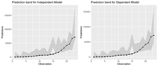
Figure 1. Prediction band for the test data under independent model and dependent model.

6. Conclusions

The Poisson distribution is generally used in compound regression models as the counting distribution. In practice, the Poisson distribution’s equi-dispersion assumption is frequently violated. The methodology presented in this paper provided a way to handle non-equi-dispersed count data in the context of compound regression models by using the CMP distribution. The proposed compound regression model can be used when the count data are over- or under-dispersed. The estimation of the parameters was carried out using a two-part GLM approach for the independent and dependent compound regression models. This approach is less complex and provides separate estimates for the count and the continuous distribution involved in the model. Since, in practice, knowledge of the actual value of the response variable rather than its predicted value is more useful, a methodology to obtain the prediction interval of the response variable was proposed. An application of the two-part GLM method to real-life data revealed that the dependent compound regression model performs relatively better than the independent compound regression model. Thus, in practice, one can start with the dependent compound regression model and look for the significance of the count variable in the model. If the count variable is found to be not significant, then the independent compound regression model can be used. To conclude, the proposed compound CMP regression model could be an alternative to modeling a compound random variable when the count data are not equi-dispersed.

References

- Gómez-Déniz, E.; Pérez-Rodríguez, J.V. Modelling distribution of aggregate expenditure on tourism. Econ. Model. 2019, 78, 293–308. [Google Scholar] [CrossRef]
- Klugman, S.A.; Panjer, H.H.; Willmot, G.E. Loss Models: From Data to Decisions; John Wiley & Sons: New York, NY, USA, 2012; Volume 715. [Google Scholar]
- Bahnemann, D. Distributions for Actuaries; Casualty Actuarial Society: Arlington, VA, USA, 2015; Volume 2. [Google Scholar]
- Jørgensen, B.; Paes De Souza, M.C. Fitting Tweedie’s compound Poisson model to insurance claims data. Scand. Actuar. J. 1994, 1994, 69–93. [Google Scholar] [CrossRef]
- Consul, P.C.; Jain, G.C. A generalization of the Poisson distribution. Technometrics 1973, 15, 791–799. [Google Scholar] [CrossRef]
- Shmueli, G.; Minka, T.P.; Kadane, J.B.; Borle, S.; Boatwright, P. A useful distribution for fitting discrete data: Revival of the Conway-Maxwell-Poisson distribution. J. R. Stat. Soc. Ser. (Appl. Stat.) 2005, 54, 127–142. [Google Scholar] [CrossRef]
- Conway, R.W.; Maxwell, W.L. A queuing model with state dependent service rates. J. Ind. Eng. 1962, 12, 132–136. [Google Scholar]
- Sellers, K.F.; Borle, S.; Shmueli, G. The COM-Poisson model for count data: A survey of methods and applications. Appl. Stoch. Model. Bus. Ind. 2012, 28, 104–116. [Google Scholar] [CrossRef]
- Sellers, K.F.; Premeaux, B. Conway-Maxwell-Poisson regression models for dispersed count data. Wiley Interdiscip. Rev. Comput. Stat. 2021, 13, e1533. [Google Scholar] [CrossRef]
- Saavithri, V.; Priyadharshini, J.; Banu, Z.P. Compound COM-Poisson Distribution with Binomial Compounding Distribution. Available online: https://www.internationaljournalssrg.org/uploads/specialissuepdf/ICRMIT/2018/MTT/ICRMIT-P122.pdf (accessed on 15 January 2023).
- Frees, E.W.; Gao, J.; Rosenberg, M.A. Predicting the frequency and amount of health care expenditures. N. Am. Actuar. J. 2011, 15, 377–392. [Google Scholar] [CrossRef]
- Andersen, D.A.; Bonat, W.H. Double generalized linear compound Poisson models to insurance claims data. Electron. J. Appl. Stat. Anal. 2017, 10, 384–407. [Google Scholar]
- Delong, Ł; Lindholm, M.; Wüthrich, M.V. Making Tweedie’s compound Poisson model more accessible. Eur. Actuar. J. 2021, 11, 185–226. [Google Scholar] [CrossRef]
- Ribeiro, E.E., Jr.; Zeviani, W.M.; Bonat, W.H.; Demétrio, C.G.; Hinde, J. Reparametrization of COM-Poisson regression models with applications in the analysis of experimental data. Stat. Model. 2020, 20, 443–466. [Google Scholar] [CrossRef]
- Jorgensen, B. The Theory of Dispersion Models; CRC Press: Boca Raton, FL, USA, 1997. [Google Scholar]
- De Jong, P.; Heller, G.Z. Generalized Linear Models for Insurance Data; Cambridge University Press: Cambridge, UK, 2008. [Google Scholar]
- Garrido, J.; Genest, C.; Schulz, J. Generalized linear models for dependent frequency and severity of insurance claims. Insur. Math. Econ. 2016, 70, 205–215. [Google Scholar] [CrossRef]
- Ribeiro, E.E., Jr. Cmpreg: Reparametrized COM-Poisson Regression Models, R Package Version 0.0.1; Available online: https://rdrr.io/github/JrEduardo/cmpreg/ (accessed on 15 January 2023).
- Dutang, C.; Charpentier, A. CASdatasets: Insurance Datasets. 2019. R Package Version 1.0-11. Available online: http://cas.uqam.ca/ (accessed on 15 January 2023).
Disclaimer/Publisher’s Note: The statements, opinions and data contained in all publications are solely those of the individual author(s) and contributor(s) and not of MDPI and/or the editor(s). MDPI and/or the editor(s) disclaim responsibility for any injury to people or property resulting from any ideas, methods, instructions or products referred to in the content. |
© 2023 by the authors. Licensee MDPI, Basel, Switzerland. This article is an open access article distributed under the terms and conditions of the Creative Commons Attribution (CC BY) license (https://creativecommons.org/licenses/by/4.0/).