The Arctan Power Distribution: Properties, Quantile and Modal Regressions with Applications to Biomedical Data

Abstract

The usefulness of (probability) distributions in the field of biomedical science cannot be underestimated. Hence, several distributions have been used in this field to perform statistical analyses and make inferences. In this study, we develop the arctan power (AP) distribution and illustrate its application using biomedical data. The distribution is flexible in the sense that its probability density function exhibits characteristics such as left-skewedness, right-skewedness, and J and reversed-J shapes. The characteristic of the corresponding hazard rate function also suggests that the distribution is capable of modeling data with monotonic and non-monotonic failure rates. A bivariate extension of the AP distribution is also created to model the interdependence of two random variables or pairs of data. The application reveals that the AP distribution provides a better fit to the biomedical data than other existing distributions. The parameters of the distribution can also be fairly accurately estimated using a Bayesian approach, which is also elaborated. To end the study, the quantile and modal regression models based on the AP distribution provided better fits to the biomedical data than other existing regression models.

1. Introduction

Parametric statistical techniques have been used in biomedical studies to conduct analyses and draw conclusions. These parametric analyses, however, are constrained by some assumptions about (probability) distributions. Thus, the task of selecting an appropriate distribution for such analyses is incredibly essential. In addition, it is nontrivial, as the use of an incorrect distribution will result in misleading inferences. Knowing which distribution to use in biomedical modeling has become increasingly important as it is used to develop new parametric regression models for modeling the relationship between endogenous variables and a set of exogenous variables. These new regression models often provide a good fit with minimal loss of information compared to the existing ones. This has triggered new interest in developing regression models using extended or modified forms of existing distributions.

Among the distributions used for developing the regression models, those that are defined on the unit interval have received much attention due to the small loss of information they offer in modeling data on this interval. Some of these distributions include the unit folded normal distribution [1], bounded truncated Cauchy power exponential distribution [2], unit exponentiated Fréchet distribution [3], log XLindley (LXL) distribution [4], unit Chen distribution [5], unit Burr XII distribution (UBXII) [6], unit generalized half-normal distribution [7], unit Burr III (UBIII) distribution [8], unit Lindley distribution [9], unit Gompertz distribution [10], unit improved second degree Lindley (UISDL) distribution [11], unit Weibull distribution [12], and exponentiated Topp–Leone distribution [13].

Despite the existence of these distributions, it is worth noting that the behavior of humans or organisms is nondeterministic, and a single distribution cannot be selected in all situations to describe or model these traits. Therefore, we develop a new distribution called the arctan power (AP) distribution for modeling data on the unit interval based on the following motivations:

• Develop a flexible unit distribution that is able to model data that are left-skewed, right-skewed, symmetric, J, and reversed-J shapes.
• Develop a unit distribution capable of modeling data with increasing, bathtub, and modified upside-down bathtub hazard rate functions (HRFs).
• Develop quantile regression for modeling response variables that are skewed or contain extreme values.
• Develop modal regression for modeling response variables that are asymmetric or heavy-tailed.

The article is organized into eight sections. Section 2 describes the development of the AP distribution. Section 3 presents their statistical properties. Section 4 shows the construction of a possible bivariate extension of the AP distribution. Nine frequentist approaches to estimating the involved parameters are proposed in Section 5. The frequentist and Bayesian univariate applications of the distribution are given in Section 6. Section 7 is devoted to the quantile and modal regressions based on the AP distribution and their applications. The conclusion of the study is presented in Section 8.

2. Development of AP Distribution

Suppose that a random variable, $X$, follows the arctan uniform (AU) distribution. Then, according to [14], the cumulative distribution function (CDF) and probability density function (PDF) of $X$ are, respectively, given by

$$F_X(x;\alpha )=\frac{\arctan (\alpha x)}{\arctan (\alpha )},\alpha >0,x\in (0,1)$$

(1)

and

$$f_X(x;\alpha )=\frac{\alpha }{\arctan (\alpha )(1+{\alpha }^2{x}^2)},x\in (0,1).$$

(2)

The proposed AP distribution is obtained using the power transformation $Y=X^{1/\beta },\beta >0$. The motivations for introducing the power parameter, $\beta$, are to improve the tail properties of the new distribution, making it capable of handling both monotonic and non-monotonic HRFs. Other researchers have used the power transformation approach to modify existing continuous distributions. See, for instance, [15,16,17]. Hence, using standard mathematical developments, the CDF of $Y$ is obtained as

$$\begin{array}{ll}{F}_Y(y;\alpha ,\beta )& =F_X(y^{\beta };\alpha )\\ & =\frac{\arctan (\alpha y^{\beta })}{\arctan (\alpha )},\alpha >0,\beta >0,y\in (0,1).\end{array}$$

(3)

The PDF and HRF are, respectively, given by

$$f_Y(y;\alpha ,\beta )=\frac{\alpha \beta y^{\beta -1}}{\arctan (\alpha )(1+{\alpha }^2{y}^{2\beta })},y\in (0,1)$$

(4)

and

$$h_Y(y;\alpha ,\beta )=\frac{\alpha \beta y^{\beta -1}}{(\arctan (\alpha )-\arctan (\alpha y^{\beta }))(1+{\alpha }^2{y}^{2\beta })},y\in (0,1).$$

(5)

Basically, when $\alpha \to 0^{+}$, the PDF of the AP distribution reduces to the one of the power distribution. As $\alpha \to 0^{+}$ and $\beta =1$, the PDF of the AP distribution reduces to the one of the standard uniform distribution. Furthermore, when $\beta =1$, the PDF of the AP distribution reduces to the one of the AU distribution.

The expanded form of the PDF is often useful when deriving the statistical properties of the distribution. Thus, using the arctangent function expansion indicated as follows: $\arctan (z)={\displaystyle \sum _{k=0}^{\infty }\frac{{(-1)}^k{z}^{2k+1}}{2k+1}},|z|<1$ (see [18]) and $\alpha \in (0,1)$, the CDF of $Y$ can be expressed as

$$F_Y(y;\alpha ,\beta )={\displaystyle \sum _{k=0}^{\infty }\frac{{(-1)}^k{\alpha }^{2k+1}{y}^{(2k+1)\beta }}{(2k+1)\arctan (\alpha )}},y\in (0,1).$$

(6)

Differentiating the expanded form of the CDF in Equation (6), the corresponding PDF is given by

$$f_Y(y;\alpha ,\beta )={\displaystyle \sum _{k=0}^{\infty }\frac{{(-1)}^k\beta {\alpha }^{2k+1}{y}^{(2k+1)\beta -1}}{\arctan (\alpha )}},y\in (0,1).$$

(7)

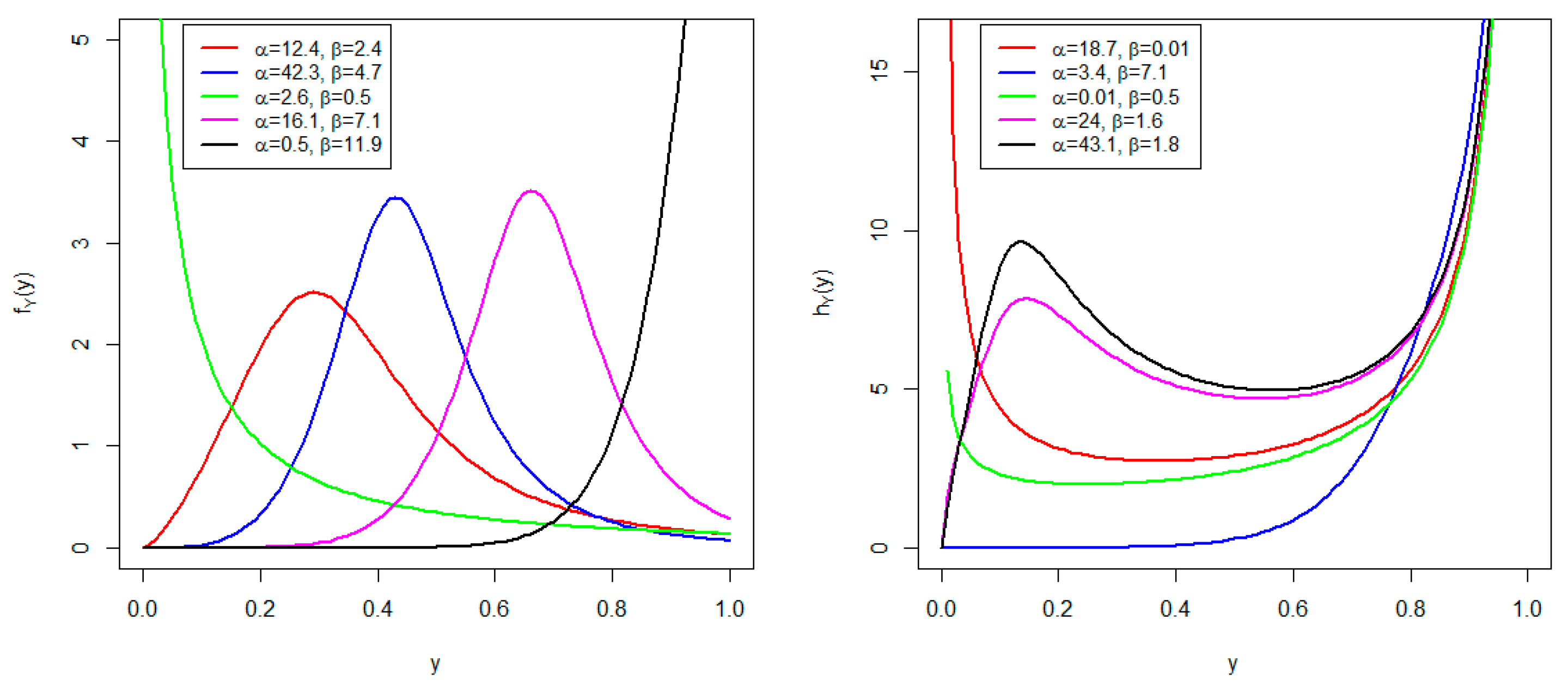
The PDF and HRF plots are shown in Figure 1 for some given parameter values. In it, the PDF exhibits left-skewed, right-skewed, J, and reversed-J shapes. This makes the AP distribution superior to the AU distribution, which exhibits only J shapes. On this side, the HRF displays increasing, bathtub, and modified upside-down bathtub shapes.

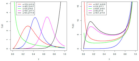
Figure 1. PDF (left) and HRF (right) plots.

3. Some Statistical Properties

In this section, some statistical properties of the AP distribution are presented.

3.1. Mode

The mode of a distribution is a useful measure of central tendency. It can be used as it for data measured on the nominal, ordinal, interval, or ratio scale. The AP distribution has a unique mode when $\beta >1$, and it is expressed in the result below.

Proposition 1.

The mode of the AP distribution is given by

$$\mathrm{mode}={\left(\frac{\beta -1}{{\alpha }^2(\beta +1)}\right)}^{\frac{1}{2\beta }},\beta >1.$$

(8)

Proof. 

To establish this expression, it is essential to locate the critical point(s) of the PDF. A critical point of the PDF is a point of the PDF, or equivalently, the logarithm of the PDF, where its derivative is zero or infinity. Taking the logarithm of the PDF and differentiating, we have

$$\frac{d\log f_Y(y;\alpha ,\beta )}{dy}=\frac{\beta -1-{\alpha }^2(\beta +1)y^{2\beta }}{y(1+{\alpha }^2{y}^{2\beta })}.$$

Equating the derivative to zero and simplifying yields the mode. This completes the proof. □

3.2. Quantile Function

The quantile function can be used to generate random observations from the AP distribution and to compute shape-related metrics like skewness and kurtosis.

Proposition 2.

The quantile function of the AP distribution is given by

$$Q(u;\alpha ,\beta )={\left[\frac{\tan (u\arctan (\alpha ))}{\alpha }\right]}^{\frac{1}{\beta }},u\in (0,1).$$

(9)

Proof. 

The quantile function is the solution $Q(u;\alpha ,\beta )$ of the following nonlinear equation: $F_Y(Q(u;\alpha ,\beta );\alpha ,\beta )=u$ for all $u\in (0,1)$. After some simplifications, letting $y=Q(u;\alpha ,\beta )$ in the CDF and equating the CDF to $u\in (0,1)$ yields the quantile function. This completes the proof. □

It is important to note that the quantile function of the AP distribution is uniquely determined with simple trigonometric and power functions.

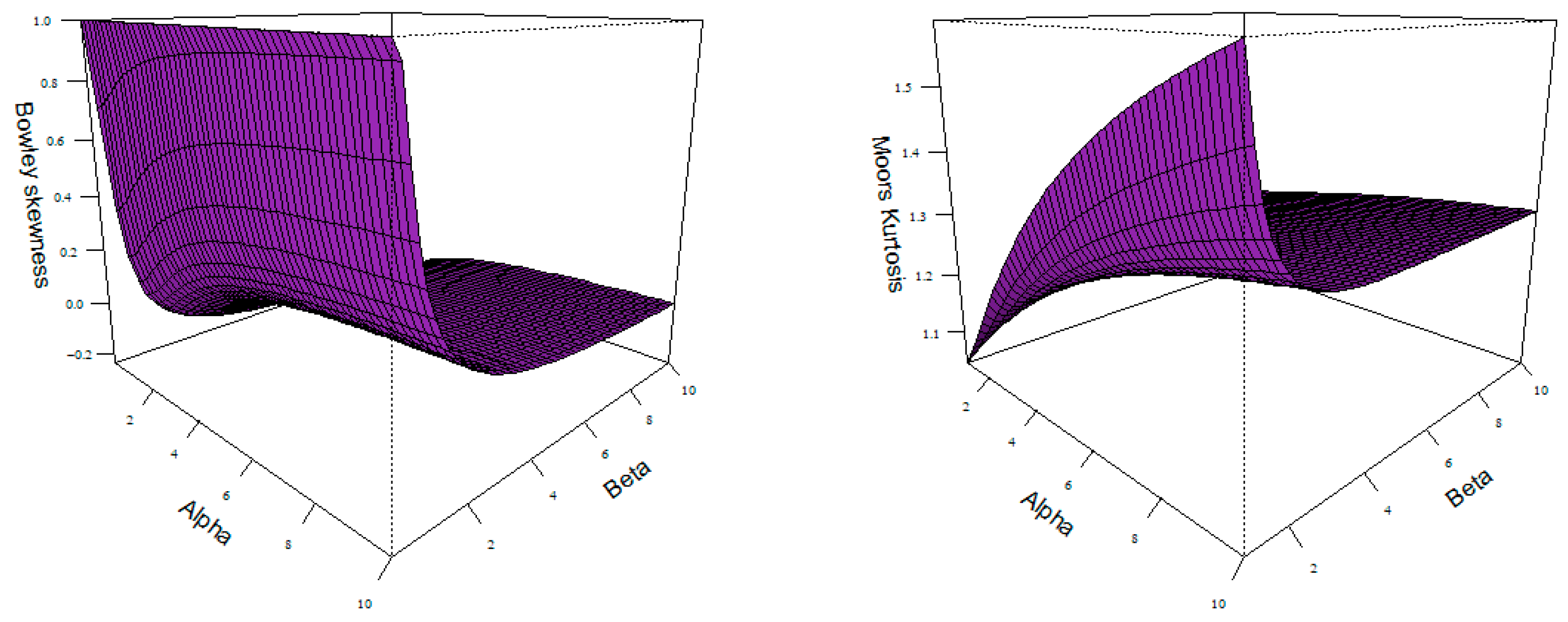
The median $Q(0.5;\alpha ,\beta )$, first quartile $Q(0.25;\alpha ,\beta )$, and upper quartile $Q(0.75;\alpha ,\beta )$ are obtained, respectively, by substituting 0.5, 0.25, and 0.75 into the quantile function. The Bowley’s (BS) measure of skewness and the Moors’ (MK) measure of kurtosis can then be calculated using the quantiles. They are, respectively, given by

$$\mathrm{BS}=\frac{Q(0.75;\alpha ,\beta )+Q(0.25;\alpha ,\beta )-2Q(0.5;\alpha ,\beta )}{Q(0.75;\alpha ,\beta )-Q(0.25;\alpha ,\beta )},$$

and

$$\mathrm{MK}=\frac{Q(0.375;\alpha ,\beta )-Q(0.125;\alpha ,\beta )+Q(0.875;\alpha ,\beta )-Q(0.625;\alpha ,\beta )}{Q(0.75;\alpha ,\beta )-Q(0.25;\alpha ,\beta )}.$$

The plots of the Bowley’s coefficient of skewness and Moor’s coefficient of kurtosis are displayed in Figure 2. Both the skewness and kurtosis are affected by changes in the values of the parameters. From this figure, we can observe that the AP distribution can be left-skewed or right-skewed.

Figure 2. Skewness (left) and Kurtosis (right) plots.

3.3. Moments and Generating Function

The moments are useful for estimating measures of central tendency, dispersion, and shapes. The generating functions can be used to estimate the moments, if they exist in the mathematical sense.

Proposition 3.

For $\alpha \in (0,1)$, the $r^{th}$raw moment of an AP random variable $Y$is given by

$${{\mu }^{\prime }}_r={\displaystyle \sum _{k=0}^{\infty }\frac{{(-1)}^k\beta {\alpha }^{2k+1}}{(r+(2k+1)\beta )\arctan (\alpha )}},r=1,2,...$$

(10)

Proof. 

The $r^{th}$ raw moment by definition is given by ${{\mu }^{\prime }}_r=E(Y^r)={\displaystyle \underset{0}{\overset{1}{\int }}{y}^r{f}_Y(y;\alpha ,\beta )dy}$. Thus, we obtain

$${{\mu }^{\prime }}_r={\displaystyle \sum _{k=0}^{\infty }\frac{{(-1)}^k\beta {\alpha }^{2k+1}}{\arctan (\alpha )}}{\displaystyle \underset{0}{\overset{1}{\int }}{y}^{r+(2k+1)\beta -1}dy}.$$

After some algebraic simplifications, the raw moment of the AP random variable is obtained. This completes the proof. □

The incomplete moment is very useful when computing measures of inequalities, such as the Lorenz and Bonferroni curves.

Proposition 4.

For $\alpha \in (0,1)$, the $r^{th}$incomplete moment of an AP random variable $Y$is given by

$${\vartheta }_r(y)={\displaystyle \sum _{k=0}^{\infty }\frac{{(-1)}^k\beta {\alpha }^{2k+1}{y}^{r+(2k+1)\beta }}{(r+(2k+1)\beta )\arctan (\alpha )}},r=1,2,...$$

(11)

Proof. 

By definition, ${\vartheta }_r(y)=E(Y^{r}1\{Y<y\})={\displaystyle \underset{0}{\overset{y}{\int }}{z}^r{f}_Y(z;\alpha ,\beta )dz}$. Hence, substituting the expanded PDF into the definition and simplifying it completes the proof. □

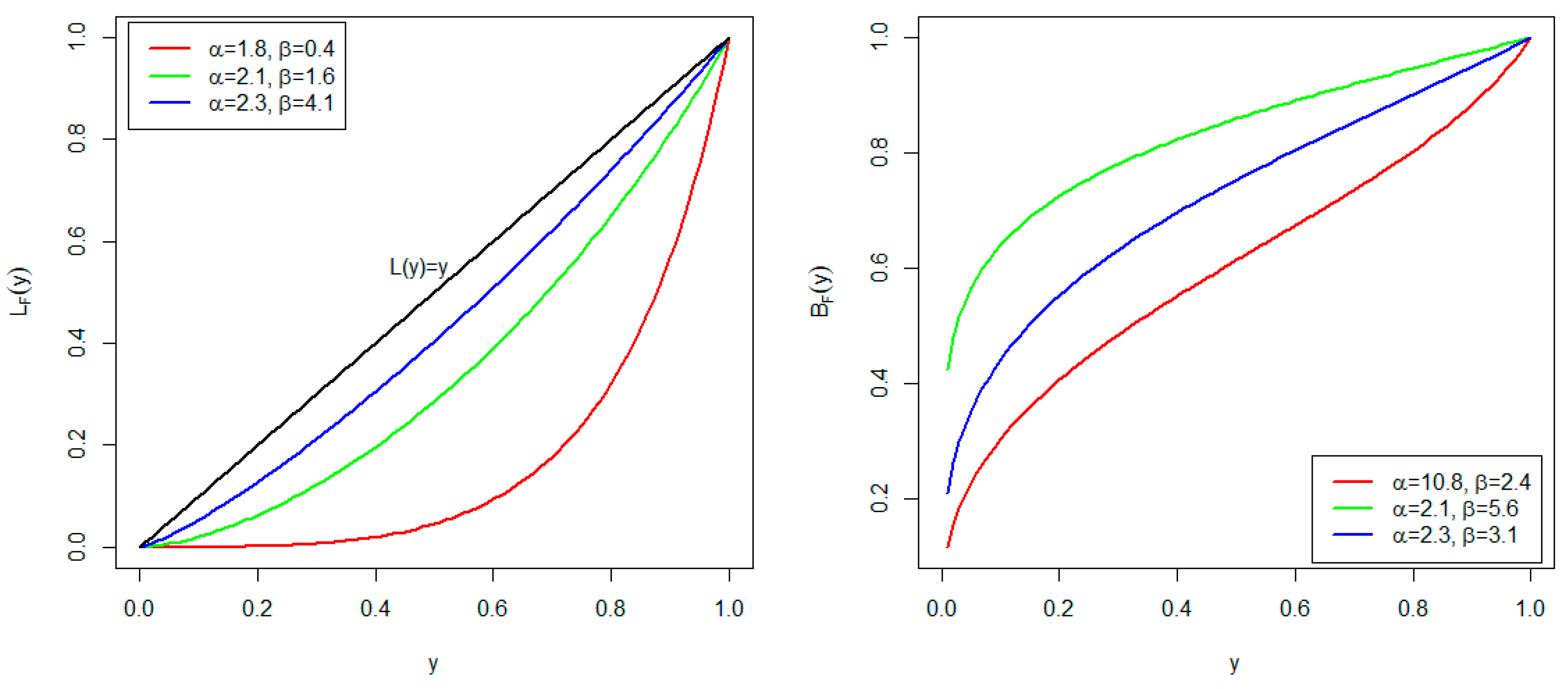
The Lorenz and Bonferroni curves are obtained, respectively, as

$$L_F(y)=\frac{1}{\mu }{\displaystyle \underset{0}{\overset{y}{\int }}z{f}_Y(z;\alpha ,\beta )dz}$$

and

$$B_F(y)=\frac{1}{\mu F_Y(y;\alpha ,\beta )}{\displaystyle \underset{0}{\overset{y}{\int }}z{f}_Y(z;\alpha ,\beta )dz},$$

where $\mu ={{\mu }^{\prime }}_1$ is the mean.

Figure 3 displays the plots of the Lorenz and Bonferroni curves of the AP distribution for some selected parameter values. For the Lorenz curve, when $L_F(y)=y$, the minimal point of inequality is obtained. When $B_F(y)=y$, the so-called equidistributional line for the Bonferroni curve is obtained.

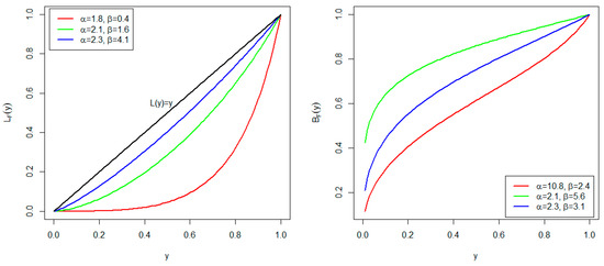
Figure 3. Plots of Lorenz curve (left) and Bonferroni curve (right).

When non-central moments of a random variable exist, they can be found using the moment-generating function (MGF).

Proposition 5.

For $\alpha \in (0,1)$, the MGF of an AP random variable $Y$is given by

$$M_Y(t)={\displaystyle \sum _{r=0}^{\infty }{\displaystyle \sum _{k=0}^{\infty }\frac{{(-1)}^k{t}^r\beta {\alpha }^{2k+1}}{r!(r+(2k+1)\beta )\arctan (\alpha )}}}.$$

(12)

Proof. 

Using the definition $M_Y(t)=E(e^{tY})={\displaystyle \underset{0}{\overset{1}{\int }}{e}^{ty}{f}_Y(y;\alpha ,\beta )}dy$ and applying the Taylor series expansion, we get

$$M_Y(t)={\displaystyle \sum _{r=0}^{\infty }\frac{t^r}{r!}}{{\mu }^{\prime }}_r$$

Hence, substituting the $r^{th}$ non-central moment completes the proof. □

3.4. Order Statistics

Order statistics are very useful in extreme value analysis. They can be used to determine the behavior of the minimum and maximum value. Consider the order statistics $Y_{1:n}\le Y_{2:n}\le \dots \le Y_{n:n}$ from the AP distribution. Then, the PDF of $Y_{k:n},k=1,2,...,n$ is

$$f_{k:n}(y;\alpha ,\beta )=C_{k:n}{\left[F_Y(y;\alpha ,\beta )\right]}^{k-1}{\left[1-F_Y(y;\alpha ,\beta )\right]}^{n-k}{f}_Y(y;\alpha ,\beta ),$$

where the factor constant is given by

$$C_{k:n}=\frac{n!}{(k-1)!(n-k)!}.$$

Using the standard binomial expansion, we can express this PDF as

$$f_{k:n}(y;\alpha ,\beta )=C_{k:n}{\displaystyle \sum _{j=0}^{n-k}{(-1)}^j\left(\begin{array}{c}n-k\\ j\end{array}\right)}{\left[F_Y(y;\alpha ,\beta )\right]}^{k+j-1}{f}_Y(y;\alpha ,\beta ).$$

Hence, we obtain

$$f_{k:n}(y;\alpha ,\beta )=\frac{\alpha \beta y^{\beta -1}{C}_{k:n}}{\arctan (\alpha )(1+{\alpha }^2{y}^{2\beta })}{\displaystyle \sum _{j=0}^{n-k}{(-1)}^j\left(\begin{array}{c}n-k\\ j\end{array}\right)}{\left[\frac{\arctan (\alpha y^{\beta })}{\arctan (\alpha )}\right]}^{k+j-1}.$$

(13)

The minimum ($Y_{1:n}$) and maximum ($Y_{n:n}$) order statistics can serve to investigate the minimum and maximum failure time of a system, respectively. The PDF of $Y_{1:n}$ is given by

$$\begin{array}{ll}{f}_{1:n}(y;\alpha ,\beta )& =n{f}_Y(y;\alpha ,\beta ){[1-F_Y(y;\alpha ,\beta )]}^{n-1}\\ & =\frac{n\alpha \beta y^{\beta -1}{(\arctan (\alpha )-\arctan (\alpha y^{\beta }))}^{n-1}}{(1+{\alpha }^2{y}^{2\beta }){(\arctan (\alpha ))}^n}\end{array}$$

and the PDF of $Y_{n:n}$ is

$$\begin{array}{ll}{f}_{n:n}(y;\alpha ,\beta )& =n{f}_Y(y;\alpha ,\beta ){[F_Y(y;\alpha ,\beta )]}^{n-1}\\ & =\frac{n\alpha \beta y^{\beta -1}{(\arctan (\alpha y^{\beta }))}^{n-1}}{(1+{\alpha }^2{y}^{2\beta }){(\arctan (\alpha ))}^n}.\end{array}$$

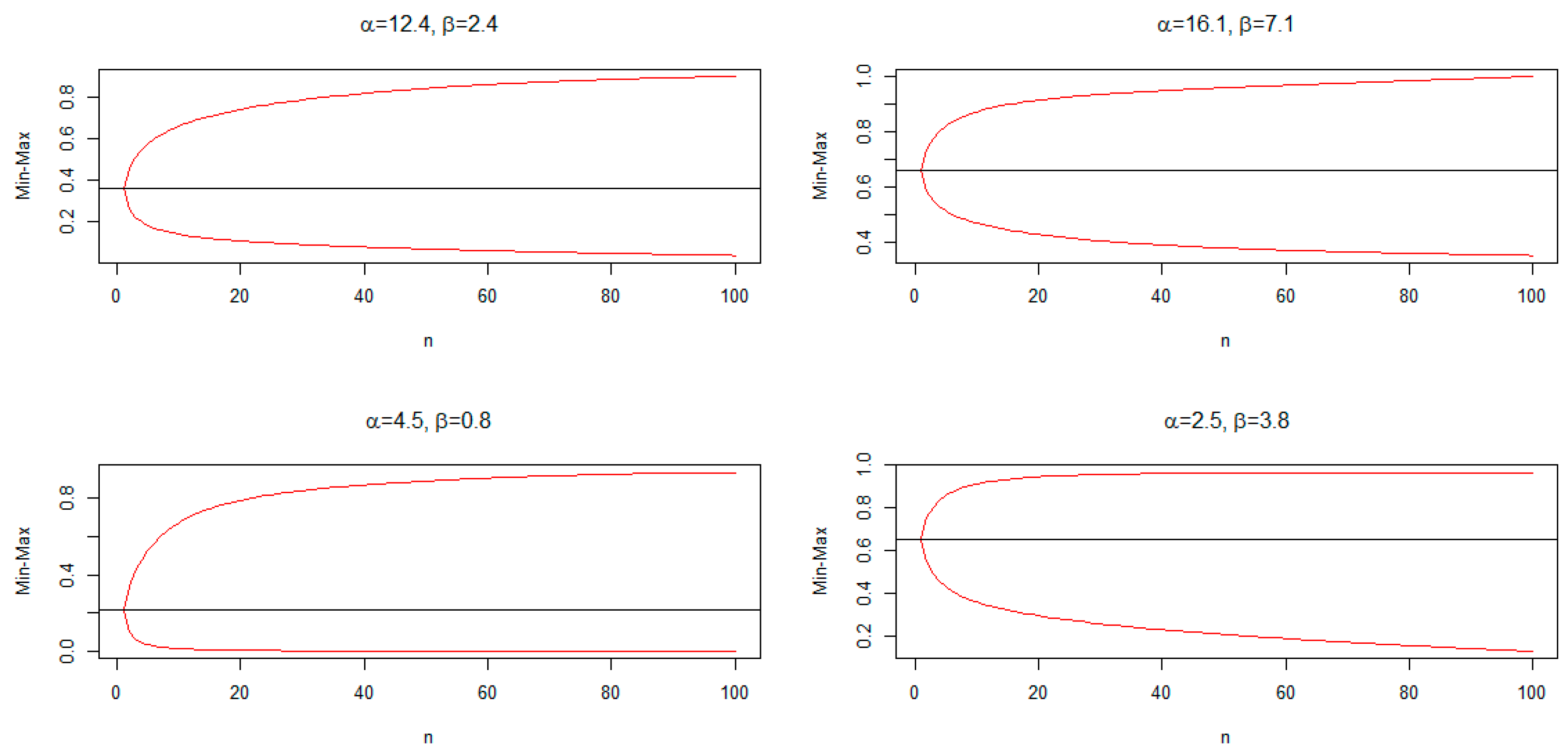
The minimum and maximum (min-max) plot of the order statistics can be used to describe whether the distribution is symmetrical or skewed. The min-max plots depend on $E(Y_{1:n})$ and $E(Y_{n:n})$. The min-max plots for some chosen parameter values for the AP distribution are shown in Figure 4. This figure reveals that the AP distribution can be right-skewed, left-skewed, or symmetric.

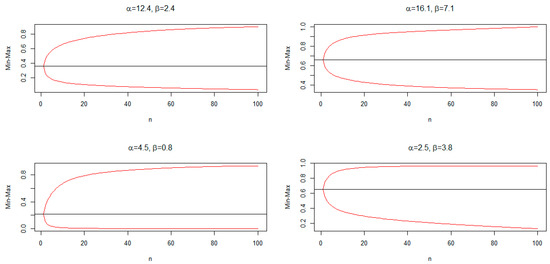
Figure 4. Min-max plots for the AP distribution.

4. Bivariate AP Distribution

The development of bivariate distributions is very useful in the context of investigating the joint relationship between two random variables. For example, one may be interested in studying the relationship between the human development index and literacy rate of a country, the maternal mortality rate and literacy rate, or rainfall and temperature, among others. There are different methods of developing bivariate distributions. One way to do this is to use copula functions (see [19]). However, in this study, we follow the approach used by [20,21]. Let $(X,Y)$ be a bivariate continuous random vector. The CDF of the bivariate AP (BAP) distribution with parameters $\alpha ,\beta ,{\rho }_1,{\rho }_2,{\rho }_3$, where $\alpha >0,\beta >0,$ $-1<{\rho }_1+{\rho }_3<1$, $-1<{\rho }_2+{\rho }_3<1,x\in (0,1)$ and $y\in (0,1)$, is given by

$$F_{XY}(x,y;\varsigma )=\frac{\arctan (\alpha x^{\beta })\arctan (\alpha y^{\beta }){(\arctan (\alpha ))}^{-2}}{{\left[1+({\rho }_1+{\rho }_3)\left(\frac{\arctan (\alpha )-\arctan (\alpha x^{\beta })}{\arctan (\alpha )}\right)+({\rho }_2+{\rho }_3)\left(\frac{\arctan (\alpha )-\arctan (\alpha y^{\beta })}{\arctan (\alpha )}\right)\right]}^{-1}},$$

(14)

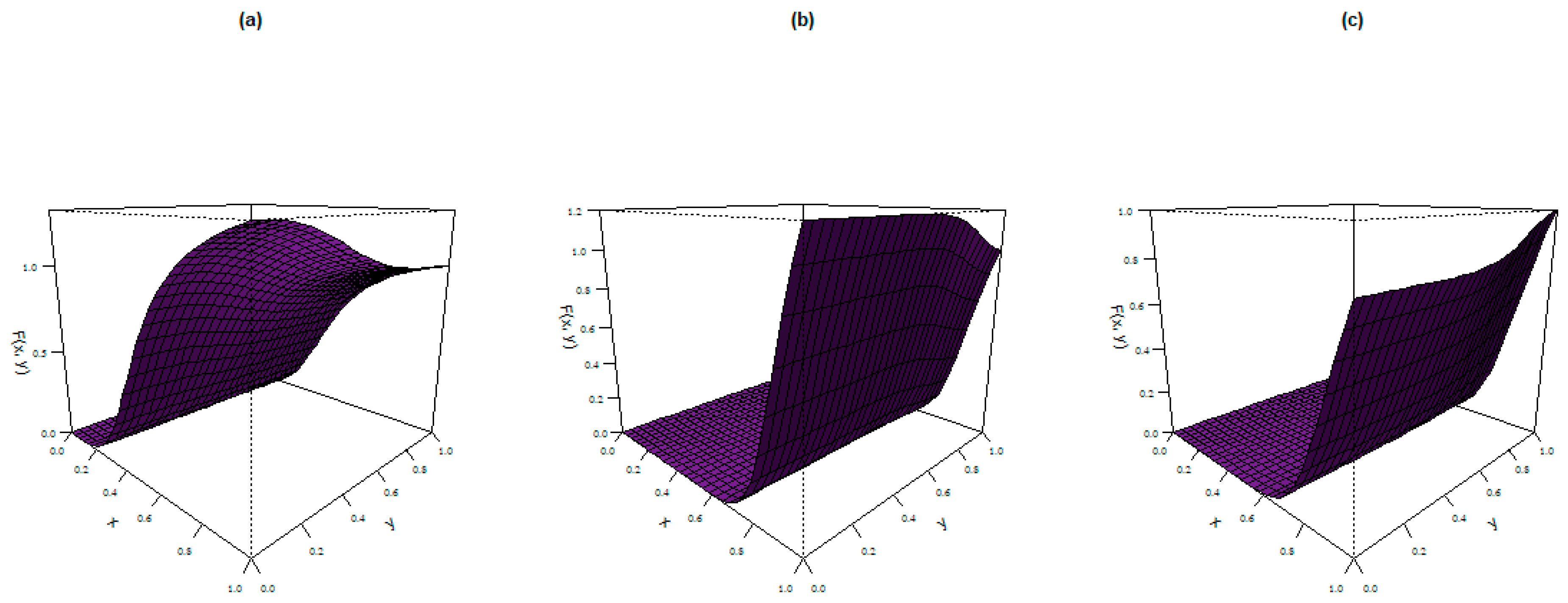
where $\varsigma =(\alpha ,\beta ,{\rho }_1,{\rho }_2,{\rho }_3)$. The plots of the CDF of the BAP distribution for the given parameter values are shown in Figure 5:

Figure 5. CDF plots of the BAP distribution.

(a)

$\alpha =8.5,\beta =2.5,{\rho }_1=0.4,{\rho }_2=0.1,{\rho }_3=0.2$,

(b)

$\alpha =4.5,\beta =8.2,{\rho }_1=-0.3,{\rho }_2=0.4,{\rho }_3=-0.2$ and

(c)

$\alpha =3.4,\beta =6.2,{\rho }_1=0.3,{\rho }_2=0.4,{\rho }_3=-0.6$.

These plots reveal different concave and convex shapes for the chosen parameter values.

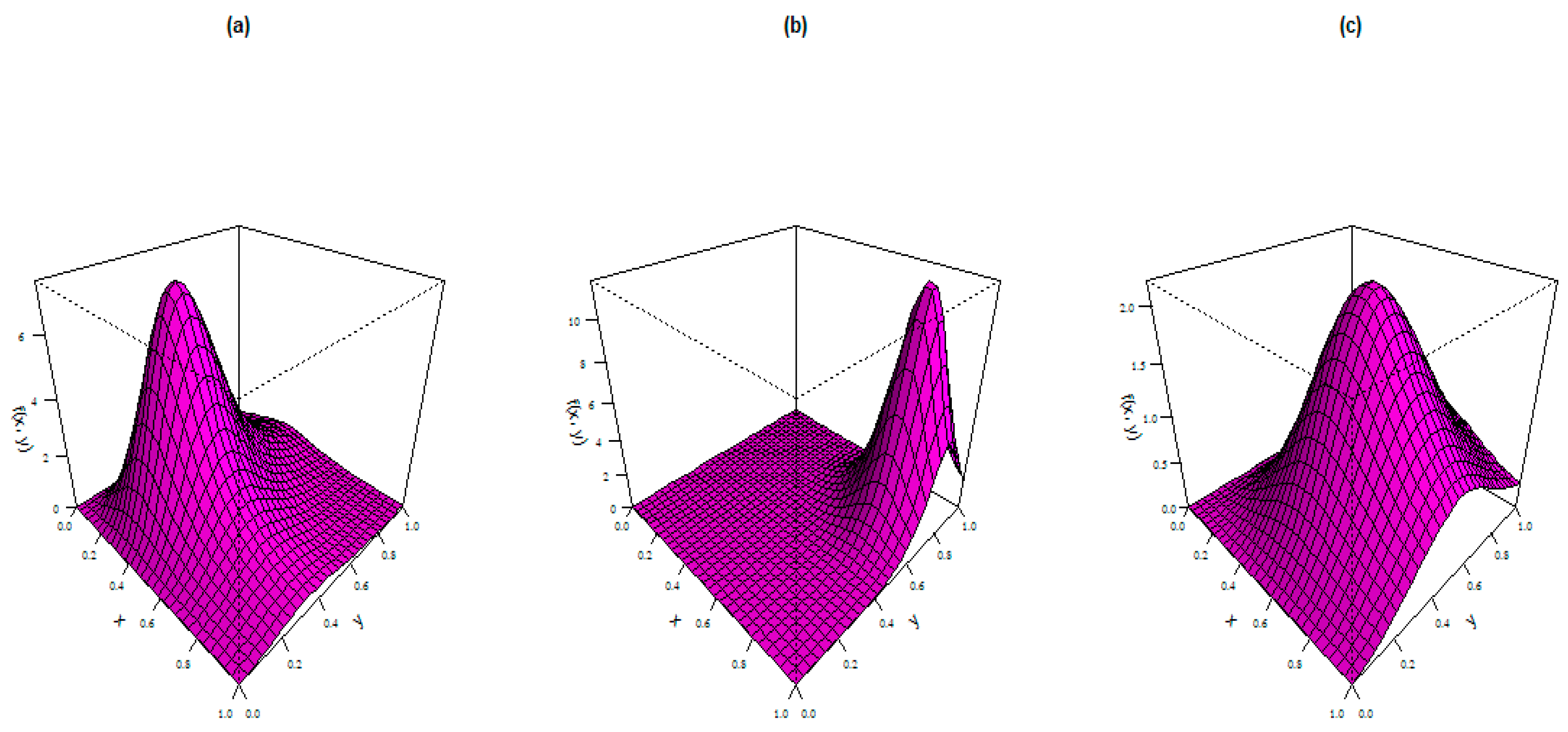
The PDF of the BAP distribution is given by

$$f_{XY}(x,y;\varsigma )=\frac{{(\alpha \beta )}^2{(xy)}^{\beta -1}{(\arctan (\alpha ))}^{-2}{[1+{(\alpha x^{\beta })}^2+{(\alpha y^{\beta })}^2+{\alpha }^4{(xy)}^{2\beta }]}^{-1}}{{\left[1+({\rho }_1+{\rho }_3)\left(\frac{\arctan (\alpha )-\arctan (\alpha x^{\beta })}{\arctan (\alpha )}\right)+({\rho }_2+{\rho }_3)\left(\frac{\arctan (\alpha )-\arctan (\alpha y^{\beta })}{\arctan (\alpha )}\right)\right]}^{-1}}.$$

(15)

The PDF plots of the BAP distribution for the following selected parameter values are displayed in Figure 6:

Figure 6. PDF plots of the BAP distribution.

(a)

$\alpha =8.5,\beta =2.5,{\rho }_1=0.4,{\rho }_2=0.1,{\rho }_3=0.2$,

(b)

$\alpha =4.5,\beta =8.2,{\rho }_1=-0.3,{\rho }_2=0.4,{\rho }_3=-0.2$ and

(c)

$\alpha =3.4,\beta =2.5,{\rho }_1=0.3,{\rho }_2=0.4,{\rho }_3=-0.6$.

These plots display left-skewed, right-skewed, and approximate symmetrical shapes.

5. Estimation Methods and Simulations

This section presents nine frequentist estimation procedures for estimating the parameters of the AP distribution. These are the maximum likelihood (ML) estimation, ordinary least squares (OLS), weighted least squares (WLS), Cramér–von Mises (CVM) estimation, Anderson–Darling (AD) estimation, percentile estimation (PE), and product spacing estimations.

5.1. Maximum Likelihood Estimation

Let $y_1,y_2,\dots ,y_n$ be independent and identically random observations of sample size $n$ from the AP distribution. Suppose that $\xi =(\alpha ,\beta {)}^{\prime }$ is the vector of parameters; then, the total log-likelihood function is

$$\ell (\xi )=n\log (\alpha \beta )-n\log (\arctan (\alpha ))+(\beta -1){\displaystyle \sum _{i=1}^n\log (y_i)}-{\displaystyle \sum _{i=1}^n\log (1+{\alpha }^2{y}_i^{2\beta })}.$$

(16)

The total likelihood function can be maximized directly with respect to the parameters $\alpha$ and $\beta$ to obtain the ML estimates of the parameters. Alternatively, these estimates can be obtained by equating the score functions to zero and solving the resulting system of equations simultaneously. The score functions, obtained by differentiating Equation (16) with respect to the parameters, are given by

$$\frac{\partial \ell (\xi )}{\partial \alpha }=\frac{n}{\alpha }-\frac{n}{(1+{\alpha }^2)\arctan (\alpha )}-{\displaystyle \sum _{i=1}^n\frac{2\alpha y_i^{2\beta }}{1+{\alpha }^2{y}_i^{2\beta }}}$$

(17)

and

$$\frac{\partial \ell (\xi )}{\partial \beta }=\frac{n}{\beta }+{\displaystyle \sum _{i=1}^n\log (y_i)}-{\displaystyle \sum _{i=1}^n\frac{2{\alpha }^2\log (y_i)y_i^{2\beta }}{1+{\alpha }^2{y}_i^{2\beta }}}.$$

(18)

The score functions do not have a closed form, thus, the resulting system of equations are solved numerically to obtain the estimates $\widehat{\alpha }$ and $\widehat{\beta }$.

5.2. Ordinary and Weighted Least Squares Estimation

Consider an ordered random sample $y_{(1)},y_{(2)},\dots ,y_{(n)}$ of size $n$ from the AP distribution; then, the OLS estimates, ${\widehat{\alpha }}_{OLS}$ and ${\widehat{\beta }}_{OLS}$, of the parameters are obtained by minimizing the function

$$OLS={{\displaystyle \sum _{i=1}^n\left(\frac{\arctan (\alpha y_{(i)}^{\beta })}{\arctan (\alpha )}-\frac{i}{n+1}\right)}}^2,$$

(19)

with respect to the parameters $\alpha$ and $\beta$. The OLS estimates can also be obtained by numerically solving the nonlinear equations

$${\displaystyle \sum _{i=1}^n\left(\frac{\arctan (\alpha y_{(i)}^{\beta })}{\arctan (\alpha )}-\frac{i}{n+1}\right)}{\pi }_s(y_{(i)};\alpha ,\beta )=0, s=1,2,$$

(20)

where

$${\pi }_1(y;\alpha ,\beta )=\frac{2y_{(i)}^{\beta }}{\arctan (\alpha )(1+{\alpha }^2{y}_{(i)}^{2\beta })}-\frac{2\arctan (\alpha y_{(i)}^{\beta })}{{(\arctan (\alpha ))}^2(1+{\alpha }^2)}$$

(21)

and

$${\pi }_2(y;\alpha ,\beta )=\frac{2y_{(i)}^{\beta }}{\arctan (\alpha )(1+{\alpha }^2{y}_{(i)}^{2\beta })}.$$

(22)

The WLS estimates, ${\widehat{\alpha }}_{WLS}$ and ${\widehat{\beta }}_{WLS}$, of the parameters are obtained by minimizing the function

$${{\displaystyle \sum _{i=1}^n\frac{{(n+1)}^2(n+2)}{i(n-i+1)}\left(\frac{\arctan (\alpha y_{(i)}^{\beta })}{\arctan (\alpha )}-\frac{i}{n+1}\right)}}^2,$$

(23)

with respect to the parameters $\alpha$ and $\beta$. Alternatively, the WLS estimates are obtained by numerically solving the nonlinear equations

$${\displaystyle \sum _{i=1}^n\frac{{(n+1)}^2(n+2)}{i(n-i+1)}\left(\frac{\arctan (\alpha y_{(i)}^{\beta })}{\arctan (\alpha )}-\frac{i}{n+1}\right)}{\pi }_s(y_{(i)};\alpha ,\beta )=0, s=1,2,$$

(24)

where ${\pi }_s(y;\alpha ,\beta ), s=1,2$ are defined in Equations (21) and (22).

5.3. Cramér–Von Mises Estimation

Given that $y_{(1)},y_{(2)},\dots ,y_{(n)}$ are the ordered observations of size $n$ from the AP distribution, the CVM estimates, ${\widehat{\alpha }}_{CVM}$ and ${\widehat{\beta }}_{CVM}$, of the parameters are obtained by minimizing the function

$$CVM=\frac{1}{12n}+{{\displaystyle \sum _{i=1}^n\left(\frac{\arctan (\alpha y_{(i)}^{\beta })}{\arctan (\alpha )}-\frac{2i-1}{2n}\right)}}^2,$$

(25)

with respect to the parameters $\alpha$ and $\beta$. The CVM estimates can also be obtained by solving the nonlinear equation

$${\displaystyle \sum _{i=1}^n\left(\frac{\arctan (\alpha y_{(i)}^{\beta })}{\arctan (\alpha )}-\frac{2i-1}{2n}\right)}{\pi }_s(y_{(i)};\alpha ,\beta )=0, s=1,2,$$

(26)

where ${\pi }_s(y;\alpha ,\beta ), s=1,2$ are given in Equations (21) and (22).

5.4. Anderson–Darling Estimation

Let $y_{(1)},y_{(2)},\dots ,y_{(n)}$ be ordered observations of size $n$ from the AP distribution. The AD estimates, ${\widehat{\alpha }}_{AD}$ and ${\widehat{\beta }}_{AD}$, of the parameters of the AP distribution are obtained by minimizing the function

$$AD=-n-\frac{1}{n}{\displaystyle \sum _{i=1}^n(2i-1)\left[\log \left(\frac{\arctan (\alpha y_{(i)}^{\beta })}{\arctan (\alpha )}\right)-\log \left(\frac{\arctan (\alpha )-\arctan (\alpha y_{(i)}^{\beta })}{\arctan (\alpha )}\right)\right]},$$

(27)

with respect to the parameters $\alpha$ and $\beta$.

5.5. Percentile Estimation

Let $y_{(1)},y_{(2)},\dots ,y_{(n)}$ be ordered observations of size $n$ from the AP distribution, and $u_i=i/(n+1)$. The percentile estimates, ${\widehat{\alpha }}_{PE}$ and ${\widehat{\beta }}_{PE}$, of the parameters of the AP distribution are obtained by minimizing the function

$$PE={\displaystyle \sum _{i=1}^n{\left[y_{(i)}-{\left(\frac{\tan (u_i\arctan (\alpha ))}{\alpha }\right)}^{1/\beta }\right]}^2},$$

(28)

with respect to the parameters $\alpha$ and $\beta$.

5.6. Product Spacing Estimations

In this subsection, the maximum product spacing (MPS) and minimum spacing distance (MSD) estimation methods are discussed. The MPS estimation method is based on the Kullback–Leibler information measure. Let us consider the uniform spacing

$$\begin{array}{ll}{D}_i& =F_Y(y_{(i)};\alpha ,\beta )-F_Y(y_{(i-1)};\alpha ,\beta )\\ & =\frac{\arctan (\alpha y_{(i)}^{\beta })}{\arctan (\alpha )}-\frac{\arctan (\alpha y_{(i-1)}^{\beta })}{\arctan (\alpha )},\end{array}$$

where $F_Y(y_{(0)};\alpha ,\beta )=0,F_Y(y_{(n+1)};\alpha ,\beta )=1$ and $D_0(\alpha ,\beta )+D_1(\alpha ,\beta )+\dots +D_{n+1}(\alpha ,\beta )=1$. The MPS estimates, ${\widehat{\alpha }}_{MPS}$ and ${\widehat{\beta }}_{MPS}$, of the parameters are obtained by directly maximizing the logarithm of the geometric mean of the spacing given by

$$MPS=\frac{1}{n+1}{\displaystyle \sum _{i=1}^{n+1}\log D_i(\alpha ,\beta )},$$

(29)

with respect to the parameters $\alpha$ and $\beta$.

The MSD estimates, ${\widehat{\alpha }}_{MSD}$ and ${\widehat{\beta }}_{MSD}$, of the parameters of the AP distribution are obtained my minimizing the function

$$MSD={\displaystyle \sum _{i=1}^n\Delta (D_i(\alpha ,\beta ),\frac{1}{n+1})},$$

(30)

where $\Delta (a,b)$ represents an appropriate distance. Several choices of $\Delta (a,b)$ exist. However, in this study, we employ the absolute $|a-b|$ and absolute-logarithm $|\log (a)-\log (b)|$ distances. Hence, the minimum spacing absolute distance (MSAD) and minimum spacing absolute-logarithm (MSALD) estimates of the parameters are obtained by minimizing the functions

$$MSAD={\displaystyle \sum _{i=1}^n|D_i(\alpha ,\beta )-\frac{1}{n+1}|}$$

(31)

and

$$MSAD={\displaystyle \sum _{i=1}^n|\log (D_i(\alpha ,\beta ))-\log (\frac{1}{n+1})|},$$

(32)

where $D_i(\alpha ,\beta )\ne \frac{1}{n+1}$ and $\log (D_i(\alpha ,\beta ))\ne \log (\frac{1}{n+1})$.

5.7. Monte Carlo Simulation

In this section, we conduct Monte Carlo simulation studies to investigate how the various estimation techniques perform with regards to estimating the parameter of the AP distribution. The exercise is carried out with two sets of parameter values, which are $\alpha =0.8,\beta =0.4$ and $\alpha =4.5,\beta =6.2$. The simulation experiments are repeated $5000$ times using the sample sizes $n=25,50,100,250$ and $350$. The average estimates (AE), average absolute bias (AB), and root mean square error (RMSE) of the parameters are estimated and reported in Table 1 and Table 2. We observe that as the sample size increases, the AE of the parameters approaches the true parameter values. Furthermore, the ABs and RMSEs of the parameters decrease as the sample size increases for all the estimation methods used. Thus, the various estimation methods produce consistent estimates for the parameters of the AP distribution. However, none of the estimation methods proves to be superior to the others.

Table 1. AE, AB, and RMSE for $\alpha =0.8$ and $\beta =0.4$.

Parameter	$\mathit{n}$	ML	MPS	OLS	WLS	AD	CVM	PE	MADS	MALDS
AE
$\alpha$	25	0.7609	1.1013	0.4303	0.5079	0.5634	0.6210	0.8969	0.1730	0.5673
	50	0.8989	1.1131	0.6865	0.7679	0.7794	0.8387	0.9400	0.1718	0.5865
	100	0.5186	0.6330	0.5285	0.5408	0.5316	0.6020	0.7364	0.3013	0.4153
	250	0.7563	0.8212	0.6438	0.6947	0.6821	0.6737	0.6598	0.4516	0.5850
	350	0.8082	0.8765	0.7720	0.8039	0.7933	0.7969	0.6947	0.5602	0.7547
$\beta$	25	0.4217	0.4674	0.3992	0.4005	0.4065	0.4237	0.4895	0.3323	0.4021
	50	0.4294	0.4580	0.4086	0.4158	0.4174	0.4258	0.4584	0.2995	0.3967
	100	0.3903	0.4039	0.3947	0.3944	0.3926	0.4016	0.4371	0.3582	0.3858
	250	0.4035	0.4115	0.3938	0.3975	0.3966	0.3974	0.4061	0.3673	0.3940
	350	0.3949	0.4026	0.3907	0.3944	0.3931	0.3936	0.3904	0.3719	0.3899
AB
$\alpha$	25	0.5584	0.6872	0.6047	0.5382	0.5453	0.6459	0.7676	0.6845	0.6637
	50	0.5308	0.6270	0.5159	0.5405	0.4941	0.5491	0.9510	0.6712	0.6083
	100	0.6628	0.6447	0.7083	0.6909	0.6867	0.6793	0.8618	0.5800	0.6805
	250	0.2803	0.2719	0.3670	0.3164	0.3256	0.3616	0.4728	0.5443	0.4994
	350	0.2584	0.2666	0.2306	0.2376	0.2389	0.2336	0.4586	0.4518	0.3332
$\beta$	25	0.0701	0.1000	0.0807	0.0724	0.0686	0.0844	0.1327	0.2182	0.1001
	50	0.0442	0.0643	0.0495	0.0435	0.0428	0.0580	0.1059	0.1275	0.0445
	100	0.0504	0.0530	0.0493	0.0493	0.0490	0.0500	0.0657	0.0640	0.0480
	250	0.0270	0.0286	0.0352	0.0306	0.0314	0.0358	0.0534	0.0557	0.0356
	350	0.0226	0.0222	0.0243	0.0176	0.0192	0.0243	0.0520	0.0428	0.0268
RMSE
$\alpha$	25	0.6832	0.8824	0.6642	0.6196	0.6373	0.7498	0.9374	0.7249	0.7684
	50	0.6291	0.7570	0.6603	0.6831	0.5963	0.7164	1.4860	0.7176	0.6671
	100	0.7322	0.7492	0.7848	0.7744	0.7611	0.7921	0.9537	0.6576	0.7420
	250	0.3359	0.3366	0.4614	0.3988	0.4108	0.4615	0.5893	0.6260	0.5625
	350	0.3129	0.3093	0.3154	0.3086	0.3098	0.3142	0.5602	0.5355	0.4107
$\beta$	25	0.0910	0.1217	0.1029	0.0918	0.0880	0.1174	0.1684	0.2464	0.1214
	50	0.0542	0.0782	0.0607	0.0559	0.0493	0.0712	0.1646	0.1592	0.0603
	100	0.0612	0.0655	0.0627	0.0618	0.0606	0.0652	0.0875	0.0981	0.0604
	250	0.0337	0.0362	0.0402	0.0364	0.0374	0.0411	0.0679	0.0696	0.0446
	350	0.0259	0.0259	0.0293	0.0242	0.0249	0.0289	0.0619	0.0560	0.0337

Table 2. AE, AB, and RMSE for $\alpha =4.5$ and $\beta =6.2$.

Parameter	$\mathit{n}$	ML	MPS	OLS	WLS	AD	CVM	PE	MADS	MALDS
AE
$\alpha$	25	7.0765	10.3643	5.9141	5.8055	6.6186	7.5983	4.8574	1.2794	8.3329
	50	5.0499	5.9801	4.8062	4.7651	4.7680	5.3690	4.1797	3.3758	5.4587
	100	4.3862	4.8383	4.1504	4.2629	4.2891	4.3589	3.9500	3.6863	4.3552
	250	4.3660	4.5560	4.2758	4.3155	4.3307	4.3597	4.1551	3.9716	4.4893
	350	4.3334	4.4767	4.2076	4.2748	4.2766	4.2668	4.2163	4.1250	4.3294
$\beta$	25	6.4914	7.3170	5.9496	5.9510	6.2163	6.5382	5.5927	3.3139	5.9368
	50	6.1885	6.6336	5.9530	6.0059	6.0516	6.2226	5.7082	4.6987	6.1925
	100	6.2534	6.5278	6.0770	6.1657	6.1849	6.2094	5.9914	5.5851	6.2811
	250	6.1297	6.2481	6.0714	6.1025	6.1135	6.1240	6.0026	5.7696	6.1201
	350	6.0608	6.1514	5.9857	6.0232	6.0258	6.0232	5.9824	5.8618	6.0932
AB
$\alpha$	25	3.4127	5.9293	3.3920	3.1570	3.4268	4.2622	2.7449	3.2862	5.8446
	50	1.8288	2.1741	2.1320	1.9167	1.7383	2.2757	1.7767	2.4817	2.5227
	100	1.0012	0.9566	1.0738	1.0249	1.0781	1.0474	1.0521	1.5290	1.2026
	250	0.8031	0.8054	0.8103	0.7709	0.7570	0.7912	0.8309	1.2029	1.0822
	350	0.6395	0.6136	0.6138	0.6133	0.6086	0.6041	0.6972	0.8890	0.5945
$\beta$	25	1.2038	1.4981	1.3240	1.2379	1.1823	1.3926	1.2174	2.9029	1.2698
	50	0.9340	0.9660	1.0599	0.9933	0.9327	1.0433	1.0666	2.1079	1.2164
	100	0.5449	0.5436	0.5723	0.5544	0.5715	0.5383	0.5769	0.9975	0.6254
	250	0.4017	0.4156	0.4049	0.4016	0.3959	0.4026	0.4575	0.7574	0.6456
	350	0.3707	0.3538	0.3835	0.3678	0.3652	0.3723	0.4190	0.5258	0.3588
RMSE
$\alpha$	25	9.0289	16.6588	7.7515	7.0825	8.9366	10.7903	5.1325	3.5862	19.9363
	50	3.1101	4.1306	3.7004	2.9429	2.7048	4.3787	2.2720	3.1047	4.0033
	100	1.2746	1.4424	1.3415	1.3020	1.3645	1.3743	1.1958	2.0602	1.7619
	250	1.0203	1.0631	1.0172	1.0052	0.9906	1.0217	1.0439	1.6323	1.3097
	350	0.7575	0.7559	0.7539	0.7476	0.7376	0.7427	0.8050	1.2130	0.7278
$\beta$	25	1.5369	2.0307	1.6441	1.5388	1.5357	1.7984	1.4325	3.3678	1.7998
	50	1.2005	1.3372	1.3614	1.2314	1.1733	1.3964	1.2318	2.6988	1.5320
	100	0.6942	0.7728	0.7270	0.6891	0.7131	0.7296	0.6689	1.5722	0.8371
	250	0.5388	0.5432	0.5306	0.5343	0.5215	0.5232	0.5916	0.9666	0.7900
	350	0.4264	0.4122	0.4673	0.4368	0.4343	0.4534	0.4743	0.6624	0.4570

6. Empirical Application

In this section, we present frequentist and Bayesian applications of the AP distribution using biomedical data.

6.1. Frequentist Application

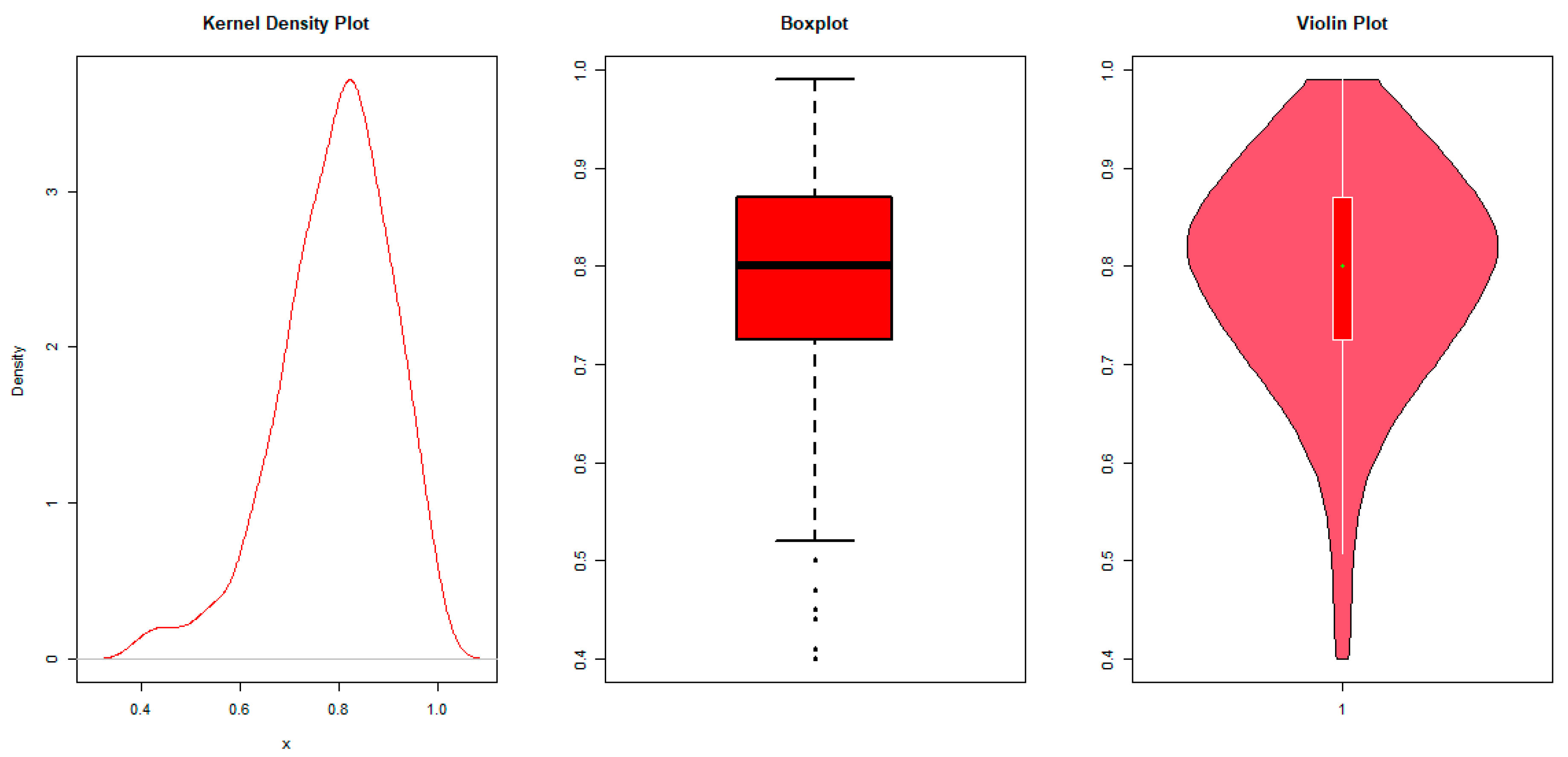
In this subsection, the univariate application of the AP distribution is illustrated using the ML estimation approach. The illustration is done using data on the recovery rates for viable CD34+ cells of 239 patients who agreed to an autologous peripheral blood stem cell (PBSC) transplant after myeloablative doses of chemotherapy between the years 2003 and 2008 at the Edmonton Hematopoietic Stem Cell Lab in the Cross Cancer Institute-Alberta Health Services. The data can be found in the simplexreg package developed by [22]. Ref. [6] recently fitted the unit Burr XII (UBXII) distribution to improve the recovery rates for viable CD34+ cells. The AP distribution is fitted to the recovery rates in this study, and its performance is compared to the AU distribution [14], unit power Weibull (UPW) distribution [23], log-XLindley (LXL) distribution [4], unit Lindley (UL) distribution [9], unit improved second degree Lindley (UISDL) distribution [11], bounded Marshall–Olkin extended exponential (BMOEE) distribution [24], unit Burr III (UBIII) distribution [8], unit Gompertz (UG) distribution [10], unit Weibull (UW) distribution [12], exponentiated Topp–Leone (ETL) distribution [13], Kumaraswamy distribution [25], and beta distribution. The performances of the distributions are compared using the log-likelihood ($\ell$), Akaike information criterion (AIC), AIC difference (DAIC), Bayesian information criterion (BIC), Anderson–Darling (AD) test, Cramér–von Mises (CVM) test, and Kolmogorov–Smirnov (KS) test. The distribution with the highest value of $\ell$ and lowest values of AIC, BIC, AD, CVM, and KS is considered to be the best. The DAIC is computed as ${\mathrm{DAIC}}_i={\mathrm{AIC}}_i-{\mathrm{AIC}}_{\min },i=1,2,...,S$, where $S$ is the number of distributions under comparison. The best distribution satisfies $\mathrm{DAIC}=0$. If $\mathrm{DAIC}>2$, then the difference in performance between the two models is significant. Before fitting the models to the recovery rate for viable CD34+ cells, we explore their characteristics. From the kernel density, boxplot, and violin plots shown in Figure 7, we observe that the recovery rate for viable CD34+ cells is left-skewed. Hence, a distribution capable of modeling left-skewed data is required, which is the case for the AP distribution.

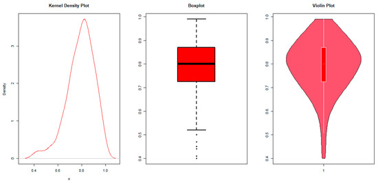
Figure 7. Kernel density, boxplot, and violin plots.

Table 3 presents the ML estimates of the parameters with their respective standard errors in brackets. The AP distribution appears to be the best model since it has the highest log-likelihood values and the smallest values for the AIC, BIC, AD, CVM, and KS. The p-values of the AD, CVM, and KS tests are given in parentheses. The p-values also indicate that the AP distribution is the best. Furthermore, looking at the DAIC values, the AP distribution significantly performs better than the other fitted distributions. Comparing the goodness-of-fit statistics of the AP and AU distributions, it can be concluded that the induction of the new parameter has greatly improved the performance of the AP distribution, making it superior to the AU distribution.

Table 3. Parameter estimates, standard errors, goodness-of-fit tests.

Model	Parameter	$\mathit{\ell }$	AIC	DAIC	BIC	AD	CVM	K-S
AP	$\alpha =5.0250(0.9841)$ $\beta =8.1856(0.6324)$	194.5900	−385.1756	0.0000	−378.2227	0.3670 (0.8806)	0.0461 (0.8999)	0.0430 (0.7694)
AU	$\alpha =2.5208\times {10}^{-14}(0.0828)$	0.0000	2.0000	387.1756	5.4765	131.0700 (<0.0001)	28.2090 (<0.0001)	0.5572 (<0.0001)
Beta	$\alpha =8.6671(0.8063)$ $\beta =2.2859(0.1962)$	191.8700	−379.7345	5.4411	−372.7816	0.8732 (0.4310)	0.1402 (0.4213)	0.0650 (0.2647)
Kumaraswamy	$\alpha =6.6942(0.4546)$ $\beta =2.4355(0.2411)$	190.7600	−377.5820	7.5936	−370.5751	1.1438 (0.2899)	0.1916 (0.2845)	0.0723 (0.1646)
UBIII	$\alpha =6.4356(0.5341)$ $\beta =1.5532(0.0695)$	192.5000	−381.0031	4.1725	−374.0501	0.7758 (0.4987)	0.1191 (0.4996)	0.0535 (0.4997)
BMOEE	$\alpha =7.6885(1.7248)$ $\beta =9.6771(0.7554)$	192.4200	−380.8355	4.3401	−373.8825	0.6848 (0.5715)	0.0866 (0.6551)	0.0489 (0.6182)
UG	$\alpha =1.0457(0.2360)$ $\beta =2.3734(0.3237)$	177.0300	−350.0612	35.1144	−343.1082	4.9419 (0.0031)	0.7829 (0.0080)	0.1106 (0.0058)
UW	$\alpha =8.0560(0.8314)$ $\beta =1.6182(0.0791)$	192.0200	−380.0314	5.1442	−373.0785	0.8636 (0.4373)	0.1328 (0.4467)	0.0557 (0.4486)
ETL	$\alpha =14.9326(1.3241)$ $\beta =0.8641(0.0718)$	192.6800	−381.3601	3.8155	−374.4072	0.6705 (0.5838)	0.0996 (0.5873)	0.0520 (0.5370)
UBXII	$\alpha =10.0760(1.0039)$ $\beta =1.7321(0.0787)$	193.5000	−383.0054	2.1702	−376.0525	0.5806 (0.6664)	0.0887 (0.6437)	0.0522 (0.5321)
UISDL	$\alpha =0.3571(0.0134)$	54.2900	−106.5865	278.5891	−103.1101	34.4330 (<0.0001)	20.1010 (<0.0001)	0.2851 (<0.0001)
UL	$\alpha =0.2424(0.0112)$	97.6400	−193.2741	191.9015	−189.7976	20.1010 (<0.0001)	4.0961 (<0.0001)	0.2365 (<0.0001)
LXL	$\alpha =4.2040(0.2569)$	154.6800	−307.3564	77.8192	−303.8799	15.7970 (<0.0001)	3.0033 (<0.0001)	0.2010 (<0.0001)
UPW	$\alpha =500.0000(8.1076\times {10}^{-6})$ $\beta =2.4183(9.9309\times {10}^{-2})$ $\lambda =0.0372(3.5461\times {10}^{-3})$	168.2600	−330.5111	54.6645	−320.0817	5.3084 (0.0021)	0.8375 (0.0059)	0.1152 (0.0035)

Figure 8 displays the histogram of the data and the estimated PDF of the AP distribution on the one hand and the empirical CDF and the estimated CDF of the AP distribution on the other hand, using the estimates of the parameter. This figure suggests that the AP distribution provides good fit to the data.

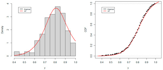
Figure 8. Histogram and estimated PDF (left), and empirical CDF and estimated CDF (right).

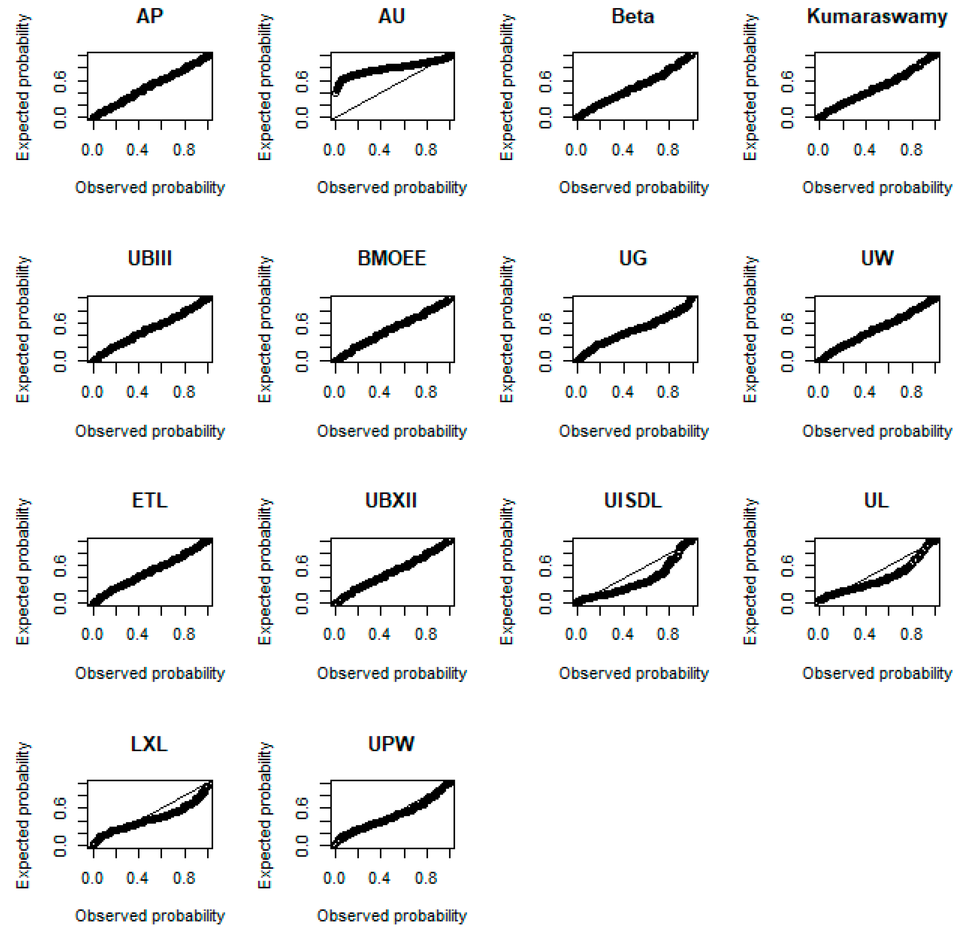
Figure 9 displays the probability-probability (P-P) plots of the fitted distributions. This figure suggests that the AP distribution provides a good fit to the data as its expected and observed probabilities cluster along the diagonal line.

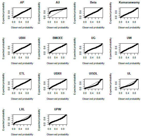
Figure 9. P-P plots of the fitted distributions.

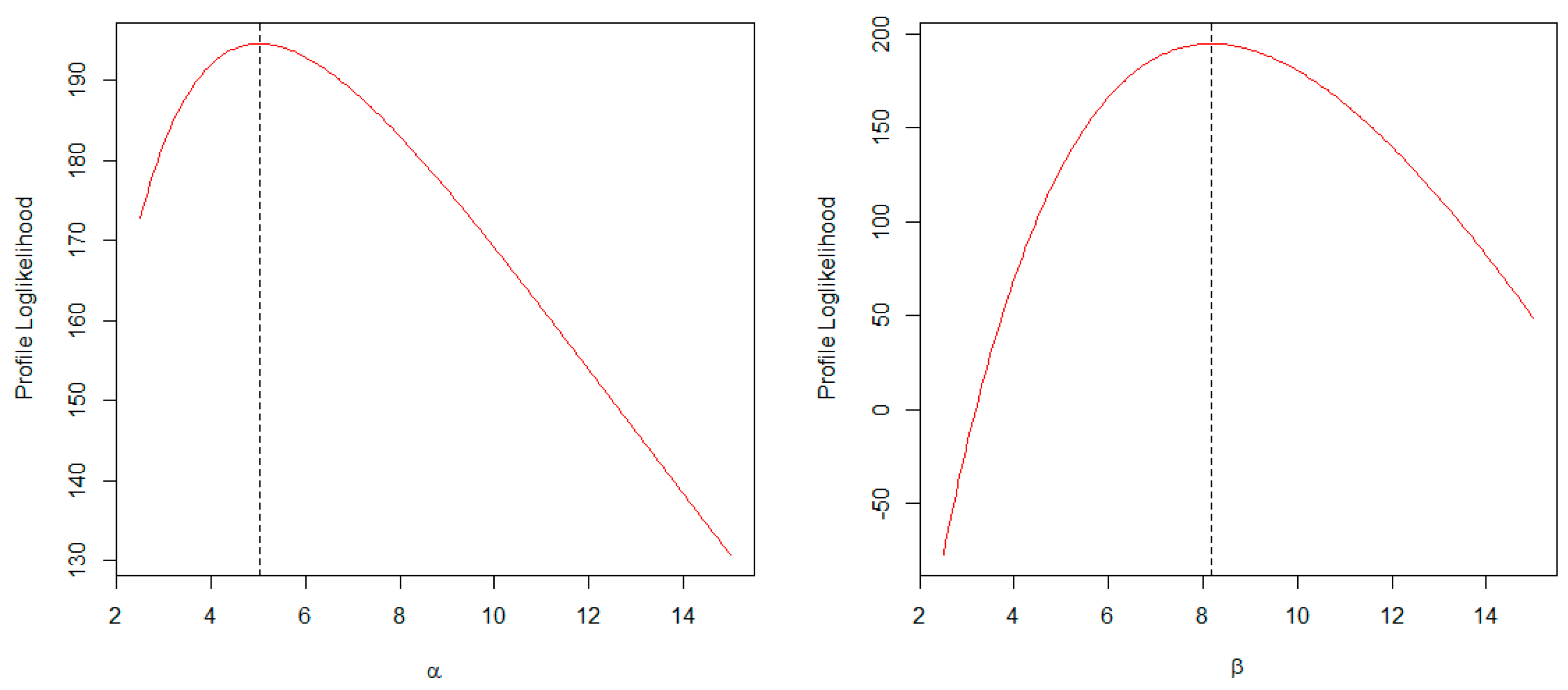
The profile log-likelihood plots of the estimated parameters of the AP distribution are shown in Figure 10. These plots suggest that the ML estimates of the parameters are unique and denote the true maxima.

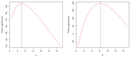
Figure 10. Profile log-likelihood plots of the estimated parameters of the AP distribution.

6.2. Bayesian Application

In this subsection, we demonstrate how to use the Bayesian approach to estimate the parameters of the AP distribution. To proceed, we need to first establish the prior distributions for the parameters, as it is very essential in Bayesian estimation. In this study, we use the non-informative gamma distribution as the prior distribution. Numerous studies have recommended the use of this approach (see [26,27]). Thus, the prior distributions of the parameters are

$$\pi (\alpha )\sim Gamma(a_1,b_1)=\frac{b_1^{a_1}}{\Gamma (a_1)}{\alpha }^{a_1-1}{e}^{-b_1\alpha },a_1>0,b_1>0,\alpha >0$$

and

$$\pi (\beta )\sim Gamma(a_2,b_2)=\frac{b_2^{a_2}}{\Gamma (a_2)}{\beta }^{a_2-1}{e}^{-b_2\beta },a_2>0,b_2>0,\beta >0$$

The joint PDF of the prior distributions of the parameters is given by

$$\pi (\alpha ,\beta )=\pi (\alpha )\pi (\beta ).$$

The joint posterior PDF is therefore given by

$$P(\alpha ,\beta |y)\propto {\displaystyle \prod _{i=1}^n{f}_Y(y_i;\alpha ,\beta )}\times \pi (\alpha ,\beta ),$$

where ${\displaystyle \prod _{i=1}^n{f}_Y(y_i;\alpha ,\beta )}$ is the likelihood function of the AP distribution. The joint posterior PDF is not analytically tractable; hence, we employ the Markov Chain Monte Carlo (MCMC) approach to obtain samples from which features of the marginal distributions can be inferred. The following hyperparameter values $a_1=a_2=b_1=b_2=0.001$ are considered for the analysis. The analysis is performed using the R2jags package in R (see [28]) and the data described in Section 6.1. We use three parallel chains, each with 40,000 iterations and a burn-in of 5000. Hence, posterior sample of size 7000 and thinning interval 5 is used in the analysis. Table 4 presents the mean estimate, Monte Carlo standard error (SE), posterior standard deviation (SD), and other numerical summaries of the posterior distribution. From the results, the MCMC algorithm has converged because the potential reduction scale factor ($\widehat{R}$) is approximately 1 and the effective sample size (neff) is greater than 400. The estimated deviance information criterion (DIC) is $-385.2000$. It can be observed that the Bayesian estimates and ML estimates of the parameters are quite close.

Table 4. Posterior summaries of the parameters of the AP distribution.

Parameter	Estimate	SE	SD	2.50%	50%	97.50%	$\widehat{\mathit{R}}$	Neff
$\alpha$	5.0600	0.0107	1.0150	3.3760	4.9540	7.3560	1.0010	5500
$\beta$	8.1600	0.0066	0.6300	6.9640	8.1490	9.4110	1.0010	6200

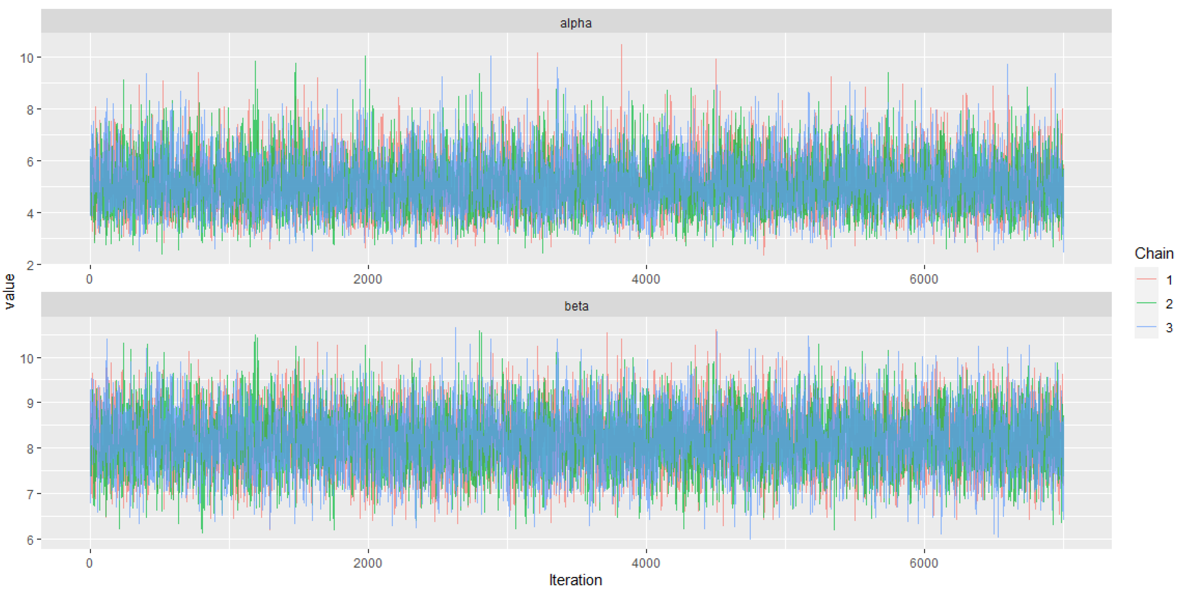
We investigate the convergence of the chains visually using the trace, ergodic mean, and autocorrelation plots. The trace plots shown in Figure 11 suggest a stationary pattern and thus convergence of the chains.

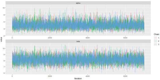
Figure 11. The AP distribution posterior parameters trace plots.

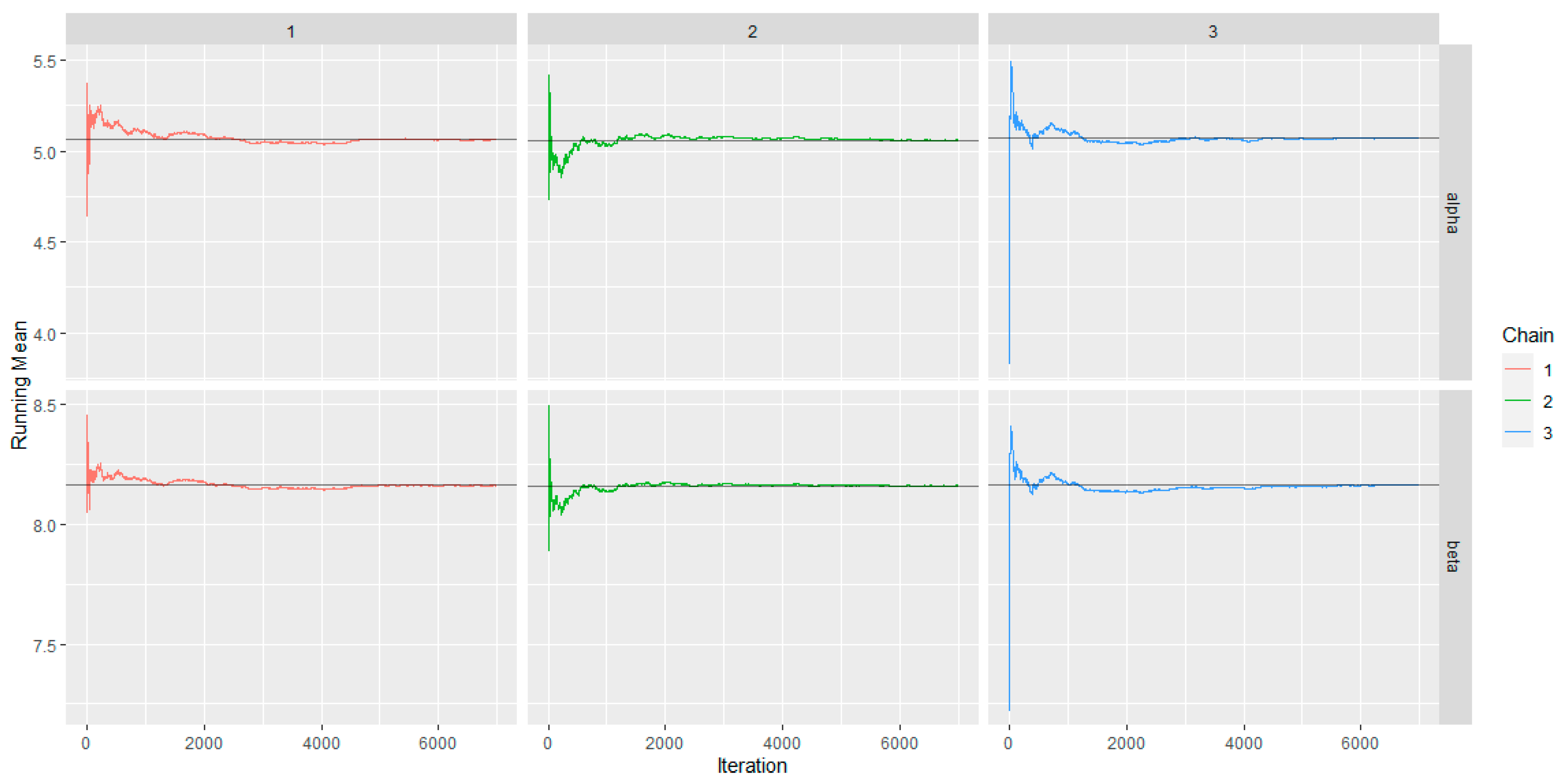
The ergodic mean plots (Figure 12) of the parameters clearly show that the chains have converged after 3000 iterations.

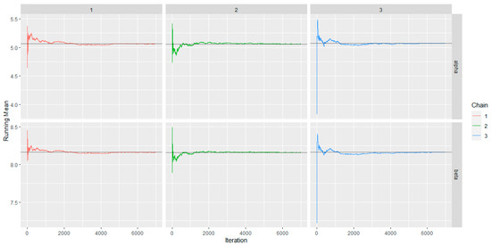
Figure 12. The AP distribution posterior parameters ergodic mean plots.

The rapid decay of the autocorrelation plots, as shown in Figure 13, suggests good mixing of the chains and the convergence of the MCMC algorithm.

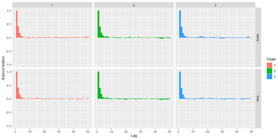
Figure 13. The AP distribution posterior parameters autocorrelation plots.

7. Regression Models

In this section, the quantile and modal regression models are developed for investigating the relationship between a dependent variable and a set of independent variable (s).

7.1. Quantile Regression Model

When investigating the influence of covariates on a skewed, bounded response variable, the beta regression model cannot produce reliable results since it models the conditional mean of the response variable. This is because the mean is not an appropriate measure of central tendency when the data are skewed. Thus, a regression model that is not influenced by outliers is required. The quantile regression is appropriate when dealing with skewed response variables. In this subsection, the AP quantile regression model is developed. To this aim, we re-parameterize the PDF of the AP distribution in terms of its quantile function. Let $\eta =Q(u;\alpha ,\beta ),\eta \in (0,1)$, making $\beta$ the subject in the quantile function, and we have $\beta ={(\log (\eta ))}^{-1}\log ({\alpha }^{-1}\tan (u\arctan (\alpha )))$. Hence, the re-parametrized PDF in terms of the quantile function is given by

$$f_Y(y;\alpha ,\eta )=\frac{\alpha {(\log (\eta ))}^{-1}\lambda y^{{(\log (\eta ))}^{-1}\lambda -1}}{\arctan (\alpha )(1+{\alpha }^2{y}^{2{(\log (\eta ))}^{-1}\lambda })},$$

(33)

where $\lambda =\log ({\alpha }^{-1}\tan (u\arctan (\alpha )))$ and $\eta$ is the quantile parameter. Suppose that $y_1,y_2,...,y_n$ are random observations from the AP distribution and $z_i$ is non-random covariates. The AP quantile regression model is thus given by

$${\eta }_i=g^{-1}({\mathit{z}}_i^{\mathrm{T}}\mathsf{\delta })$$

where $\mathsf{\delta }={({\delta }_0,{\delta }_1,{\delta }_2,\dots ,{\delta }_p)}^{\mathrm{T}}$ is the vector of coefficients of the covariates to be estimated, ${\mathit{z}}_i^{\mathrm{T}}=(1,z_{i1},z_{i2},\dots ,z_{ip})$ is the known $i^{th}$ vector of independent variables, and $g(\cdot )$ is an appropriate link function that relates the independent variables to the conditional quantile of the dependent variable. When $u=0.5$, the median regression is obtained. Although different link functions exist for modeling bounded response variables, in this study, the logit link function is used due to the easy interpretation of the parameters. Hence, we have

$$\log \left(\frac{{\eta }_i}{1-{\eta }_i}\right)={\delta }_0+{\delta }_1{z}_{i1}+{\delta }_2{z}_{i2}+\dots +{\delta }_p{z}_{ip}$$

The log-likelihood for estimating the parameters of the regression model is

$$\begin{array}{l}\ell =n\log (\alpha )-n\log (\arctan (\alpha ))+n\log (\lambda )-{\displaystyle \sum _{i=1}^n\log (}\log ({\eta }_i))+{\displaystyle \sum _{i=1}^n({(\log ({\eta }_i))}^{-1}\lambda -1)\log (y_i)}\\ -{\displaystyle \sum _{i=1}^n\log (1+{\alpha }^2{y}_i^{2{(\log ({\eta }_i))}^{-1}\lambda })}.\end{array}$$

(34)

Maximizing the log-likelihood function in Equation (34) with respect to the involved parameters gives the estimates of the parameters of the model. For more information on the development of parametric quantile regressions, we refer the readers to [2,3,6].

7.2. Modal Regression

When the response variable is heavy-tailed or asymmetric, modal regression is known to give a better fit than the conditional mean or median regression [29]. It is also established that the prediction intervals from modal regression possess a higher coverage probability than the mean-based prediction interval (see [29,30]). This subsection presents the modal-based regression using the AP distribution. Suppose that the transformation $(\alpha ,\beta )\to (\eta ,\phi )$ is one-to-one, where $\eta \in (0,1)$ is the mode and $\phi >1$ is a precision/shape parameter. Then the PDF of the AP distribution can be re-parameterized in terms of the mode (see [29]). Let $\beta =\phi$, then $\alpha ={\eta }^{-\phi }{(\phi +1)}^{-1/2}{(\phi -1)}^{1/2}$ and the PDF of the AP distribution in terms of mode is given by

$$f_Y(y;\eta ,\phi )=\frac{{\eta }^{-\phi }\phi {(\phi +1)}^{-1/2}{(\phi -1)}^{1/2}{y}^{\phi -1}}{\arctan ({\eta }^{-\phi }{(\phi +1)}^{-1/2}{(\phi -1)}^{1/2})(1+{\eta }^{-2\phi }{(\phi +1)}^{-1}(\phi -1)y^{2\phi })}.$$

(35)

The modal regression is given by

$${\eta }_i=h^{-1}({\mathit{z}}_i^{\mathrm{T}}\mathsf{\delta })$$

where $\mathsf{\delta }={({\delta }_0,{\delta }_1,{\delta }_2,\dots ,{\delta }_p)}^{\mathrm{T}}$ is the vector of unknown parameters to be estimated, ${\mathit{z}}_i^{\mathrm{T}}=(1,z_{i1},z_{i2},\dots ,z_{ip})$ are the known $i^{th}$ vector of covariates and $h(\cdot )$ is an appropriate link function that links the covariates to the conditional mode of the response variable. The logit link function is adopted since the mode of the AP distribution lies on (0, 1). Thus, we have

$$\log \left(\frac{{\eta }_i}{1-{\eta }_i}\right)={\delta }_0+{\delta }_1{z}_{i1}+{\delta }_2{z}_{i2}+\dots +{\delta }_p{z}_{ip}$$

The log-likelihood for estimating the parameters of the model is given by

$$\begin{array}{l}\ell =n\log (\phi {(\phi +1)}^{-1/2}{(\phi -1)}^{1/2})-\phi {\displaystyle \sum _{i=1}^n\log ({\eta }_i)}+(\phi -1){\displaystyle \sum _{i=1}^n\log (y_i)}-{\displaystyle \sum _{i=1}^n\log (\arctan ({\eta }_i^{-\phi }{(\phi +1)}^{-1/2}{(\phi -1)}^{1/2}))}-\\ {\displaystyle \sum _{i=1}^n\log (1+{\eta }_i^{-2\phi }{(\phi +1)}^{-1}(\phi -1)y_i^{2\phi })}.\end{array}$$

(36)

The estimates of the parameters of the modal regression are obtained by maximizing Equation (36) with respect to the involved parameters.

7.3. Residual Analysis

Investigating how well a model fits a given data set is very important. Hence, the adequacy of the model is often examined using the residuals from the fitted model. The Cox–Snell and randomized quantile residuals are used to assess the performance of the regression models in this study.

Thus, the Cox–Snell residuals (see [31]) are used to assess the adequacy of the regression models. The Cox–Snell residuals are defined as

$$e_i=-\log (1-F_Y(y_i;\widehat{\mathsf{\delta }}),i=1,2,...,n$$

where $\widehat{\mathsf{\delta }}$ is the vector of the estimated parameters of the regression models. The Cox–Snell residuals are expected to be standard exponentially distributed if the models provide good fit to the data.

Assessing the randomized quantile residuals of the model is another alternative for examining the adequacy of the regression model. The randomized quantile residual is given by

$$e_i={\Phi }^{-1}(F_Y(y_i;\widehat{\mathsf{\delta }}),i=1,2,...,n,$$

where ${\Phi }^{-1}(\cdot )$ is the quantile of the standard normal distribution. If the regression model provides good fit to the data, the randomized quantile residuals are expected to follow the standard normal distribution (see [32]).

7.4. Monte Carlo Simulation for Regression Models

In this section, Monte Carlo simulation experiments are carried out to assess how the ML estimates perform with regards to estimating the parameters of the AP quantile and modal regressions. The simulations for the quantile regression are carried out using the conditional median. The conditional median in this case is the median of the response variable given the values of the covariates. The experiment is replicated 5000 times for each sample size $n=50,150,250,350,450$, and $550$. For the first scenario, the following parameter combinations are used for the quantile and modal regressions, respectively: $({\delta }_0,{\delta }_1,{\delta }_2,\alpha )=(0.8,0.3,0.6,1.5)$ and $({\delta }_0,{\delta }_1,{\delta }_2,\phi )=(0.8,0.3,0.6,1.5)$. In the second scenario, the parameter following combinations are used, respectively, for the quantile and modal regressions: $({\delta }_0,{\delta }_1,{\delta }_2,\alpha )=(0.1,0.4,0.8,1.3)$ and $({\delta }_0,{\delta }_1,{\delta }_2,\phi )=(0.1,0.4,0.8,1.3)$. The following regression structure with two covariates is employed during the simulation for both regression models:

$$\log \left(\frac{{\eta }_i}{1-{\eta }_i}\right)={\delta }_0+{\delta }_1{z}_{i1}+{\delta }_2{z}_{i2},i=1,2,...,n.$$

The covariate, $z_{i1}$, is generated from a standard normal distribution and $z_{i2}$ is from a $t$ distribution with four degrees of freedom. The covariates are held fixed during the simulation process. The observations for the response variable are generated using the inversion method for both the quantile and modal regressions. The performance of the estimation method is assessed using the average estimate (AE), absolute bias (AB), and root mean square error (RMSE). The results in Table 5 and Table 6 reveal that the AEs approach the true parameter values as the sample size increases. Furthermore, the ABs and RMSEs decrease as the sample size increases. Hence, the estimates of the parameters for both models are consistent based on the ML technique.

Table 5. Simulation results for the first scenario.

Parameter	$\mathit{n}$	AP Quantile Regression			Parameter	$\mathit{n}$	AP Modal Regression
		AE	AB	RMSE			AE	AB	RMSE
${\delta }_0$	50	0.7659	0.2028	0.2533	${\delta }_0$	50	0.6495	0.5931	0.6372
	150	0.7870	0.1286	0.1586		150	0.7551	0.5240	0.5771
	250	0.7837	0.1041	0.1304		250	0.7015	0.4583	0.5226
	350	0.7953	0.0896	0.1104		350	0.7526	0.4226	0.4880
	450	0.7990	0.0868	0.1071		450	0.7674	0.3745	0.4419
	550	0.7990	0.0681	0.0844		550	0.7668	0.3499	0.4195
${\delta }_1$	50	0.4010	0.3256	0.3983	${\delta }_1$	50	0.7202	0.6676	0.7959
	150	0.3266	0.1974	0.2407		150	0.6208	0.5630	0.7027
	250	0.3308	0.1737	0.2122		250	0.6470	0.5746	0.7074
	350	0.3119	0.1443	0.1742		350	0.5695	0.5176	0.6518
	450	0.3012	0.1403	0.1711		450	0.5439	0.4813	0.6098
	550	0.2951	0.1044	0.1309		550	0.4965	0.4450	0.5669
${\delta }_2$	50	0.6015	0.0893	0.1157	${\delta }_2$	50	0.5921	0.3502	0.4263
	150	0.6045	0.0480	0.0614		150	0.6143	0.2171	0.2787
	250	0.6057	0.0381	0.0469		250	0.6090	0.1694	0.2232
	350	0.6006	0.0325	0.0410		350	0.6183	0.1563	0.2020
	450	0.6001	0.0291	0.0371		450	0.6174	0.1259	0.1659
	550	0.6017	0.0272	0.0336		550	0.6187	0.1193	0.1569
$\alpha$	50	1.8184	0.7279	0.8795	$\phi$	50	1.6644	0.2465	0.2948
	150	1.6469	0.4111	0.5266		150	1.5793	0.1477	0.1879
	250	1.5957	0.3058	0.3971		250	1.5376	0.1026	0.1333
	350	1.5689	0.2526	0.3190		350	1.5289	0.0840	0.1100
	450	1.5586	0.2227	0.2891		450	1.5216	0.0721	0.0931
	550	1.5412	0.2047	0.2602		550	1.5085	0.0693	0.0870

Table 6. Simulation results for the second scenario.

Parameter	$\mathit{n}$	AP Quantile Regression			Parameter	$\mathit{n}$	AP Modal Regression
		AE	AB	RMSE			AE	AB	RMSE
${\delta }_0$	50	0.1667	0.1496	0.1906	${\delta }_0$	50	0.3746	0.3802	0.6027
	150	0.1484	0.1207	0.1502		150	0.3336	0.3336	0.5220
	250	0.1136	0.0907	0.1097		250	0.2376	0.2422	0.3747
	350	0.1171	0.0845	0.1021		350	0.2302	0.2282	0.3570
	450	0.1164	0.0842	0.1028		450	0.2165	0.2085	0.3172
	550	0.1122	0.0714	0.0856		550	0.1841	0.1748	0.2572
${\delta }_1$	50	0.4049	0.3025	0.3523	${\delta }_1$	50	0.5759	0.5815	0.6773
	150	0.3681	0.1882	0.2312		150	0.4728	0.4831	0.5746
	250	0.4042	0.1654	0.2011		250	0.4892	0.4385	0.5127
	350	0.3862	0.1498	0.1808		350	0.4187	0.3793	0.4540
	450	0.3912	0.1453	0.1771		450	0.4457	0.3684	0.4586
	550	0.3730	0.1047	0.1324		550	0.3974	0.3408	0.4147
${\delta }_2$	50	0.7935	0.1038	0.1363	${\delta }_2$	50	0.8970	0.3344	0.4124
	150	0.8057	0.0546	0.0699		150	0.8773	0.2046	0.2720
	250	0.8013	0.0426	0.0519		250	0.8651	0.1441	0.2004
	350	0.8008	0.0364	0.0457		350	0.8471	0.1296	0.1734
	450	0.7987	0.0327	0.0414		450	0.8440	0.1052	0.1468
	550	0.8050	0.0326	0.0394		550	0.8339	0.1025	0.1397
$\alpha$	50	1.2087	0.3183	0.4361	$\phi$	50	1.4403	0.2164	0.2713
	150	1.2667	0.2281	0.2932		150	1.3604	0.1242	0.1589
	250	1.2719	0.1967	0.2448		250	1.3258	0.0870	0.1127
	350	1.2930	0.1702	0.2034		350	1.3211	0.0700	0.0911
	450	1.2871	0.1632	0.1971		450	1.3153	0.0609	0.0785
	550	1.2919	0.1546	0.1845		550	1.3063	0.0588	0.0739

7.5. Application of Regression Models

The use of quantile and modal regressions is demonstrated in this subsection. The application of the quantile regression is illustrated via the conditional median regression by setting $u=0.5$. The application of the models is illustrated by regressing the recovery rates for viable CD34+ cells of 239 patients described in Section 6 on the following covariates: gender ($z_{i1}$, 0 for female and 1 for male), chemotherapy ($z_{i2}$, 0 for receiving chemotherapy on a one-day protocol and 1 for a three-day protocol), and adjusted patient’s age ($z_{i3}$, that is the current age minus 40). Ref. [6] fitted the UBXII median regression with the following results: $\mathrm{AIC}=-384.2649$ and $\mathrm{BIC}=-366.8826$. The authors showed that the UBXII median regression performs better than the Kumaraswamy median regression with the following results: $\mathrm{AIC}=-375.6599$ and $\mathrm{BIC}=-358.2775$, and beta mean regression with the following results: $\mathrm{AIC}=-381.7912$ and $\mathrm{BIC}=-364.4089$. The exploratory analysis in Section 6.1 suggests that the response variable is left-skewed or contains some extreme values. This is an indication that robust regression models are required for modeling the data, and thus our choice of using the median and modal regressions is appropriate. We adopt the following regression structure:

$$\log \left(\frac{{\eta }_i}{1-{\eta }_i}\right)={\delta }_0+{\delta }_1{z}_{i1}+{\delta }_2{z}_{i2}+{\delta }_3{z}_{i3},i=1,2,...,239$$

to model the data. Table 7 displays the estimates of the model parameters, standard errors, p-values, and information criteria. From the information criteria, the AP regressions (median and modal) perform better than the UBXII median, Kumaraswamy median, and beta mean regressions. Since $\mathrm{DAIC}>2$, the AP regressions perform significantly better than the compared regressions. Comparing the AP median regression with the modal regression, it can be said that the AP median regression performs better than the modal regression. From Table 7, it can be seen that the parameter ${\delta }_1$ is not statistically significant at 5% level of significance. Hence, the variable gender has no significant effect on the recovery rate. The parameters ${\delta }_2$ and ${\delta }_3$ are statistically significant at the 5% level of significance. This implies that the recovery rate of older patients is higher than that of younger ones. Furthermore, the recovery rate of patients who receive chemotherapy on a three-day protocol is higher than that of those who receive chemotherapy on a one-day protocol.

Table 7. Estimates, standard errors, and information criteria for the regression models.

AP Quantile Regression				AP Modal Regression
Parameter	Estimate	Standard Error	p-Value	Parameter	Estimate	Standard Error	p-Value
${\delta }_0$	1.0119	0.1226	<0.0001	${\delta }_0$	0.8903	0.1715	<0.0001
${\delta }_1$	0.0533	0.0912	0.5585	${\delta }_1$	0.0921	0.1235	0.4560
${\delta }_2$	0.2392	0.0940	0.0110	${\delta }_2$	0.3153	0.1559	0.0432
${\delta }_3$	0.0169	0.0049	0.0006	${\delta }_3$	0.0253	0.0082	0.0020
$\alpha$	5.6100	1.1128	<0.0001	$\phi$	8.4244	0.6471	<0.0001
		$\ell =201.1400$				$\ell =199.7300$
		$\mathrm{AIC}=-392.2835$				$\mathrm{AIC}=-389.4540$
		$\mathrm{BIC}=-374.9012$				$\mathrm{BIC}=-372.0717$

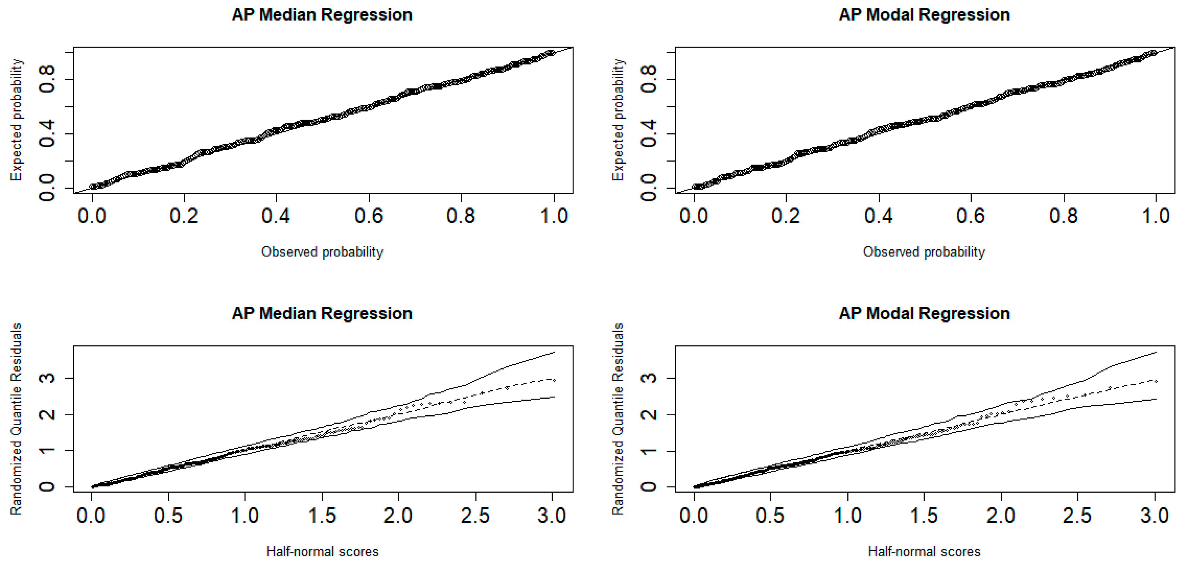
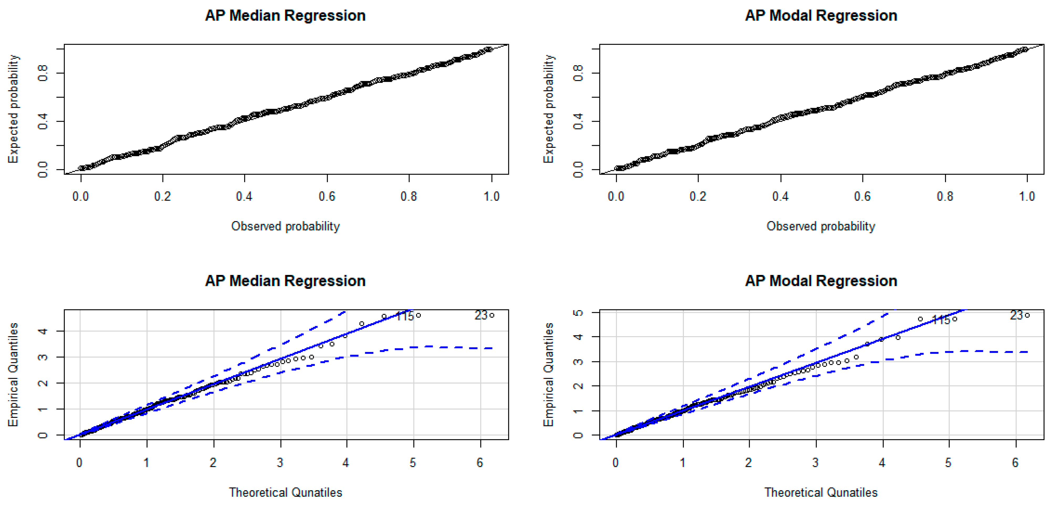
The adequacy of the fitted regression models is assessed by examining the residuals of the fitted models. The P-P plots and half-normal plots with simulated envelopes of the randomized quantile residuals in Figure 14 indicate that the models are adequate.

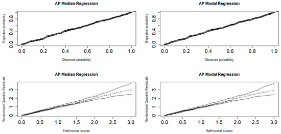
Figure 14. P-P (top) and half-normal (bottom) plots of the randomized quantile residuals.

The P-P and quantile-quantile (Q-Q) plots with simulated envelopes of the Cox–Snell residuals shown in Figure 15 again affirm that the fitted models are adequate.

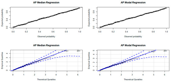
Figure 15. P-P (top) and Q-Q (bottom) plots of the Cox–Snell residuals.

8. Conclusions

In this study, the AP distribution and its associated quantile and modal regressions were developed. The PDF of the AP distribution exhibits flexible shapes such as left-skewed, right-skewed, J, and reversed-J shapes. This makes the distribution a suitable candidate for fitting data with such characteristics. The corresponding HRF also suggests that the distribution is capable of fitting data with monotonic and non-monotonic failure rates. We explored the performance of nine frequentist estimation procedures for estimating the parameters of the distribution using Monte Carlo simulations, and the results revealed that most of the procedures are consistent with regards to estimating the parameters. A biomedical application of the distribution showed that the model provides a good fit to the data. A Bayesian illustration of how to apply the distribution showed that the approach is able to estimate the parameters of the distribution very well. The applications of the elaborated quantile and modal regressions demonstrated that the new regression models outperformed some existing regression models. The future perspective of this work is to demonstrate the Bayesian applications of the quantile and modal regressions.

References

- Korkmaz, M.Ç.; Chesneau, C.; Korkmaz, Z.S. The unit folded normal distribution: A new unit probability distribution with the estimation procedures, quantile regression modeling and educational attainment applications. J. Reliab. Stat. Stud. 2022, 15, 261–298. [Google Scholar] [CrossRef]
- Nasiru, S.; Abubakari, A.G.; Chesneau, C. New lifetime distribution for modeling data on the unit interval: Properties, application and quantile regression. Math. Comput. Appl. 2022, 27, 105. [Google Scholar] [CrossRef]
- Abubakari, A.G.; Luguterah, A.; Nasiru, S. Unit exponentiated Fréchet distribution: Actuarial measures, quantile regression and applications. J. Indian Soc. Probab. Stat. 2022, 23, 387–424. [Google Scholar] [CrossRef]
- Eliwa, M.S.; Ahsan-ul-Haq, M.; Al-Bossly, A.; El-Morshedy, M. Properties and estimation techniques with application to model data from SC16 and P3 algorithms. Math. Probl. Eng. 2022, 2022, 9289721. [Google Scholar] [CrossRef]
- Korkmaz, M.Ç.; Emrah, A.; Chesneau, C.; Yousof, H.M. On the unit-Chen distribution with associated quantile regression and applications. Math. Slovaca 2022, 72, 765–786. [Google Scholar] [CrossRef]
- Korkmaz, M.Ç.; Chesneau, C. On the unit Burr XII distribution with the quantile regression modeling and applications. Comput. Appl. Math. 2021, 40, 29. [Google Scholar] [CrossRef]
- Korkmaz, M.Ç. The unit generalized half normal distribution: A new bounded distribution with inference and application. UPB Sci. Bull. Ser. A 2020, 82, 133–140. [Google Scholar]
- Modi, K.; Gill, V. Unit Burr-III distribution with application. J. Stat. Manag. Syst. 2019, 23, 579–592. [Google Scholar] [CrossRef]
- Mazucheli, J.; Menezes, A.F.B.; Chakraborty, S. On the one parameter unit-Lindley distribution and its associated regression model for proportion data. J. Appl. Stat. 2019, 46, 700–714. [Google Scholar] [CrossRef]
- Mazucheli, J.; Menezes, A.F.; Dey, S. Unit-Gompertz distribution with applications. Statistica 2019, 79, 25–43. [Google Scholar]
- Altun, E.; Cordeiro, G.M. The unit-improved second-degree Lindley distribution: Inference and regression modeling. Comput. Stat. 2019, 35, 259–279. [Google Scholar] [CrossRef]
- Mazucheli, J.; Menezes, A.F.; Ghitany, M.E. The unit Weibull distribution and associated inference. J. Appl. Probab. Stat. 2018, 13, 1–22. [Google Scholar]
- Pourdarvish, A.; Mirmostafaee, S.M.T.K.; Naderi, K. The exponentiated Topp-Leone distribution: Properties and application. J. Appl. Environ. Biol. Sci. 2015, 5, 251–256. [Google Scholar]
- Kharazmi, O.; Alizadeh, M.; Contreras-Reyes, J.E.; Haghbin, H. Arctan-based family of distributions: Properties, survival regression, Bayesian analysis and applications. Axioms 2022, 11, 399. [Google Scholar] [CrossRef]
- Al-Mofleh, H.; Afify, A.Z.; Ibrahim, N.A. A new extended two-parameter distribution: Properties, estimation methods and, applications in medicine and geology. Mathematics 2020, 8, 1578. [Google Scholar] [CrossRef]
- Iqbal, Z.; Tahir, M.M.; Riaz, N.; Ali, S.A.; Ahmad, M. Generalized inverted Kumaraswamy distribution: Properties and application. Open J. Stat. 2017, 7, 645–662. [Google Scholar] [CrossRef]
- Iqbal, Z.; Hasnain, S.A.; Salman, M.; Ahmad, M.; Hamedani, G.G. Generalized exponentiated moment exponential distribution. Pak. J. Stat. 2014, 30, 537–554. [Google Scholar]
- Gradshteyn, I.S.; Ryzhik, I.M. Tables of Integrals, Series and Products, 7th ed.; Elsevier/Academic Press: Amsterdam, The Netherlands, 2007. [Google Scholar]
- Sklar, A. Random variables, joint distribution functions and copulas. Kybernetika 1973, 9, 449–460. [Google Scholar]
- Elhassanein, A. On statistical properties of a new bivariate modified Lindley distribution with an application to financial data. Complexity 2022, 2022, 2328831. [Google Scholar] [CrossRef]
- Ganji, M.; Bevrani, H.; Hami, N. A new method for generating continuous bivariate families. J. Iran. Stat. Soc. 2018, 17, 109–129. [Google Scholar] [CrossRef]
- Zhang, P.; Qiu, Z.; Shi, C. Simplexreg: An R package for regression analysis of proportional data using the simplex distribution. J. Stat. Softw. 2016, 71, 1–21. [Google Scholar] [CrossRef]
- Bantan, R.A.R.; Shafiq, S.; Tahir, M.H.; Elhassanein, A.; Jamal, F.; Almutiry, W.; Elgarhy, M. Statistical analysis of COVID-19 data: Using a new univariate and bivariate statistical model. J. Funct. Spaces 2022, 2022, 2851352. [Google Scholar] [CrossRef]
- Ghosh, I.; Dey, S.; Kumar, D. Bounded M-O extended exponential distribution with applications. Stoch. Qual. Control. 2019, 34, 35–51. [Google Scholar] [CrossRef]
- Kumaraswamy, P. A Generalized probability density function for double-bounded random processes. J. Hydrol. 1980, 46, 79–88. [Google Scholar] [CrossRef]
- Muse, A.H.; Chesneau, C.; Ngesa, O.; Mwalili, S. Flexible parametric accelerated hazard model: Simulation and application to censored lifetime data with crossing survival curves. Math. Comput. Appl. 2022, 27, 104. [Google Scholar] [CrossRef]
- Khan, S.A. Exponentiated Weibull regression for time-to-event data. Lifetime Data Anal. 2018, 24, 328–354. [Google Scholar] [CrossRef]
- Su, Y.S.; Yajima, M. R2jags: A Package for Running Jags from R. 2012. Available online: https://CRAN.R-project.org/package=R2jags (accessed on 21 December 2022).
- Menezes, A.F.B.; Mazucheli, J.; Chakraborty, S. A collection of parametric modal regression models for bounded data. J. Biopharm. Stat. 2021, 31, 490–506. [Google Scholar] [CrossRef]
- Yao, W.; Li, L. A new regression model. Scand. J. Stat. 2014, 41, 656–671. [Google Scholar] [CrossRef]
- Cox, D.R.; Snell, E.J. A general definition of residuals. J. R. Stat. Soc. Ser. B 1968, 30, 248–275. [Google Scholar] [CrossRef]
- Dunn, P.K.; Smyth, G.K. Randomized quantile residuals. J. Comput. Graph. Stat. 1996, 5, 236–244. [Google Scholar]
Disclaimer/Publisher’s Note: The statements, opinions and data contained in all publications are solely those of the individual author(s) and contributor(s) and not of MDPI and/or the editor(s). MDPI and/or the editor(s) disclaim responsibility for any injury to people or property resulting from any ideas, methods, instructions or products referred to in the content. |
© 2023 by the authors. Licensee MDPI, Basel, Switzerland. This article is an open access article distributed under the terms and conditions of the Creative Commons Attribution (CC BY) license (https://creativecommons.org/licenses/by/4.0/).