Stability Analysis of Caputo Fractional Order Viral Dynamics of Hepatitis B Cellular Infection

Abstract

We present a Caputo fractional order mathematical model that describes the cellular infection of the Hepatitis B virus and the immune response of the body with Holling type II functional response. We study the existence of unique positive solutions and the local and global stability of virus-free and endemic equilibria. Finally, we present numerical results using the Adam-type predictor–corrector iterative scheme.

1. Introduction

Hepatitis B is a known killer infectious disease caused by the Hepatitis B virus (HBV), which attacks the liver cells (Hepatocyte), resulting in changes in the antigen structure of the surface of the liver cells, thus, leading to attack and destruction by a mechanism called ‘self-mediated immune damage’.

Although “recovered” patients have lifetime protective immunity, tiny levels of HBV DNA can still be discovered occasionally. These traces of HBV DNA are infectious and stimulate HBV-specific B- and T-cell responses, which control viremia [1]. However, HBV replication is strongly suppressed by the antiviral effects of inflammatory cytokines generated by HBV-specific $CD8+$ T lymphocytes when they detect the antigen in the infected or transgenic liver, as shown in chimpanzee [2] and transgenic mouse [3].

Hepatitis B infection is in two phases; acute and chronic. The acute stage is the earliest stage of the infection whereby the body can recover by its immune system within six $\left(6\right)$ months. The acute infection stage might be asymptotic and characterized by viral replication. Loss of appetite, joint and muscle discomfort, low-grade fever, and potential stomach aches are all signs of an acute infection. Recovery from acute HBV infection means that the virus is no longer in the bloodstream, but inactive in the liver. However, if one uses immune-suppressing drugs, the virus in your liver might be reactivated in the future. HBV replicates only within the host cell since it lacks the enzymes necessary for protein and nucleic acid synthesis [4]. Chronic HBV infection occurs when the virus is still detectable six months after the infection, indicating that the virus has not been fully cleared by the immune system and is still present in the patient’s blood and liver. The majority of patients with chronic infections are asymptomatic. HBV is transmitted from an infected person to an uninfected person through sexual transmission, child-birth relation, misuse of contaminated needles such as syringes, exchange of infected body fluids such as blood, saliva, menstrual, seminal, and vaginal fluid [5].

It is also well-known that infected people do not always show symptoms in the early stages, although some may experience an acute illness that lasts several weeks, including Jaundice (yellowing of the skin and eye), dark urine, and extreme fatigue, nausea, vomiting, and some abdominal pains. Despite the above symptoms mentioned, symptoms exhibited by patients also depend on the status of the immune system of the patient, the age, and general health of the patient [4].

Due to the severity of hepatitis B infection, it has intrigued many scientists and researchers to investigate the dynamics of HBV. In [6], a spatio-temporal dynamics of a fractional model for HBV infection with cellular immunity was proposed. A time-fractional diffusion model for HBV infection with capsids and Cytotoxic T lymphocytes (CTL) immune response and were able to show that the diffusion and the order of fractional derivatives in the sense of Caputo do not affect the stability of the equilibria, but they can affect the time to arrive at the equilibria. When the order of the fractional derivative increases, for example, the model’s solutions converge quickly to the equilibrium points.

In [7], the authors looked at a fractional-order HBV immunological model’s global analysis and simulation. Using the Lyapunov function to prove the model’s stability, they derived basic reproduction numbers and presented their relationship with the corresponding equilibria. Studying the hepatitis B virus, the authors in [8] incorporated the immune response and took into account both cytolytic and noncytolytic effect pathways. The dynamics of immune response to hepatitis B, which takes into account contributions from innate and adaptive immune responses, as well as cytokines, has also been studied, see, [9].

In this article, we consider an HBV model with a Holling type 2 functional response rate and three (3) compartments, i.e., healthy hepatocytes (H), infected hepatocytes (I), and the body’s immune response (R). We study the existence and uniqueness of the solutions and the equilibrium states, i.e., virus-free and endemic equilibrium state. When the virus present in the liver cells exceeds the cytokines, the virus will overcome the cytokines and multiply in the body, resulting in an endemic state where the virus comes to stay in the body. When cytokines outnumber the viruses in the body, the viruses are cleared from the body, and the person is virus-free.

The rest of the paper is organized as follows; Section 2 presents preliminary results for fractional calculus. We present the fractional order model and the analysis in Section 3. In Section 4, we present the local and global stability analysis. The numerical results and simulations are presented in Section 5. Finally, we present the conclusions in Section 6.

2. Mathematical Preliminary on Fractional Calculus

In this section, we present useful results from the theory of fractional calculus; see, for example, the monographs [10,11] for further details.

Definition 1 

([11]). The fractional order integral of the function $f:[0,+\infty )\to \mathbb{R})$ of order $\alpha \in (0,1)$ is defined in the sense of Riemann–Liouville as where $[0,T]\subset {\mathbb{R}}_{+}.$ Then fractional integral of order v for a function g in the sense of Riemann–Liouville is defined as

$${\mathcal{I}}^{\alpha }f\left(t\right)=\frac{1}{\mathrm{\Gamma }\left(\alpha \right)}{\int }_0^t{(t-\tau )}^{\alpha -1}f\left(\tau \right)\mathrm{d}\tau ,t>0,$$

(1)

where $[0,T]\subset {\mathbb{R}}^{+}$ and $\mathrm{\Gamma }\left(\alpha \right)={\int }_0^{\infty }{t}^{\alpha -1}{e}^{-t}dt,\alpha >0,$ is the Euler gamma function.

Definition 2 

([11]). For a function $f\in C^n([0,+\infty ],\mathbb{R}),$ the Caputo fractional-order derivative of order α is defined by

$${}^c{D}^{\alpha }f\left(t\right)=\frac{1}{\mathrm{\Gamma }(n-\alpha )}={\int }_0^t{(t-\tau )}^{n-\alpha -1}{f}^{\left(n\right)}\left(\tau \right)\mathrm{d}\tau ,t>0,$$

(2)

where $n=\lfloor \alpha \rfloor +1$ and $\lfloor \alpha \rfloor$ denotes the smallest integer that is less or equal to $\alpha .$

Finally, a relation between 1 and 2 is given by

Lemma 1. 

Let $\alpha \ge 0$ and $n=\lfloor \alpha \rfloor +1.$ Then

$${\mathcal{I}}^{\alpha }{(}^c{D}^{\alpha }f\left(t\right))=f\left(t\right)-\sum _{k=0}^{n-1}\frac{f^k\left(0\right)}{k!}{t}^k.$$

In particular, if $0<\alpha \le 1,$ then

$${\mathcal{I}}^{\alpha }{(}^c{D}^{\alpha }f\left(t\right))=f\left(t\right)-f\left(0\right).$$

The generalized mean value theorem for the Caputo fractional order is given by

Lemma 2. 

For $\alpha \in (0,1],$ let $f\left(t\right)\in C\left(\right[a,b\left]\right)$ and $D^{\alpha }f\left(t\right)\in (a,b].$ Then it holds

$$f\left(t\right)=f\left(a\right)+{\displaystyle \frac{1}{\mathrm{\Gamma }\left(\alpha \right)}}{D}^{\alpha }f\left(\eta \right){(t-a)}^{\alpha },0\le \eta \le t,t\in (a,b].$$

(3)

3. Fractional Order Model Derivation and Analysis

We consider a liver consisting of Healthy Hepatocyte $\left(H\right),$ Infected hepatocytes $\left(I\right)$, and immune response-dependent cytotoxic cells $\left(R\right).$ We assume a logistic growth of healthy hepatocytes, see, e.g., [12,13]. Healthy Hepatocytes of the liver are known to have half-lives of more than six months; see, [14]. In the presence of the Hepatitis B virus, we assume that the rate at which hepatocytes become infected is proportional to $HI.$ Given $\beta$ as the contact rate and assuming that infected hepatocytes die at a rate ${\mu }_1,$ the dynamic model for the infected hepatocytes and the immune response can be described as

$$\begin{array}{cc}\hfill \frac{dH}{dt}& =r_{1}H\left(1-{\displaystyle \frac{H}{K}}\right)-\beta HI,\hfill \\ \hfill \frac{dI}{dt}& =\beta HI-c_{1}RI-{\mu }_{1}I,\hfill \\ \hfill \frac{dR}{dt}& =\delta HI+{\displaystyle \frac{r_{2}RI}{\sigma +I}}-c_{2}RI-{\mu }_{2}R,\hfill \end{array}$$

(4)

with the initial conditions $H\left(0\right)=H_0\ge 0,I\left(0\right)=I_0\ge 0$ and $R\left(0\right)=R_0\ge 0,$ where $c_1$ and $c_2$ are the rates of deactivation of virons and cytotoxic cells, respectively. Let $\delta$ be the rate of production of cytotoxic cells, and ${\mu }_2$ be the baseline degradation rate. We note that the immune response of the cytotoxic cells to the viral invasion was included via a positive feedback mechanism, with a response term ${\displaystyle \frac{r_{2}RI}{\sigma +I}}$ which is a saturating function of the amount of virus present, the full description of the parameters can be seen in Table 1. Following [15,16], the fractional order model of the mathematical model (4) is given by Caputo derivativeas follows

$$\begin{array}{cc}\hfill {}^C{D}_t^{\alpha }H& =r_1^{\alpha }H\left(1-{\displaystyle \frac{H}{K}}\right)-{\beta }^{\alpha }HI,\hfill \\ \hfill {}^C{D}_t^{\alpha }I& ={\beta }^{\alpha }HI-c_1^{\alpha }RI-{\mu }_1^{\alpha }I,\hfill \\ \hfill {}^C{D}_t^{\alpha }R& ={\delta }^{\alpha }HI+{\displaystyle \frac{r_2^{\alpha }RI}{{\sigma }^{\alpha }+I}}-c_2^{\alpha }RI-{\mu }_2^{\alpha }R,\hfill \end{array}$$

(5)

subject to the initial conditions $H\left(0\right)=H_0\ge 0,I\left(0\right)=I_0\ge 0$ and $R\left(0\right)=R_0\ge 0,$ where ${}^C{D}^{\alpha }$ denotes Caputo fractional derivative with the order of the derivative $\alpha \in (0,1].$

Table 1. The parameters involved in the model equation are described in detail (5).

Parameters	Description
$\beta$	Contact rate (rate of infection of the normal cell)
${\mu }_1$	Natural death rate of HBV
${\mu }_2$	Natural death rate of Cytotoxic cell
$\delta$	Production rate of Cytotoxic cells
$\sigma$	Cytotoxic cell simulation half saturation rate
$r_1$	Growth rate of uninfected hepatocytes
$r_2$	Rate simulation of Cytotoxic cells by HBV
$c_1$	Rate of destruction of HBV by Cytotoxic cells
$c_2$	Rate of deactivation of Cytotoxic cells by HBV
K	Carrying capacity
${\mathcal{R}}_0$	Basic reproduction Number
$\alpha$	Fractional order

3.1. Qualitative Properties

Here, we study the well-posedness of the fractional order model. By means of a Banach contraction mapping, we the existence and uniqueness of the solutions.

Let $X\left(t\right)={(H,I,R)}^T$ and $\mathcal{K}{(t,X\left(t\right))}^T={\left({\varphi }_i\right)}^T,i=1,2,3,$ where,

$$\begin{array}{cc}\hfill {\varphi }_1& =r_1^{\alpha }H\left(1-{\displaystyle \frac{H}{K}}\right)-{\beta }^{\alpha }HI,\hfill \\ \hfill {\varphi }_2& ={\beta }^{\alpha }HI-c_1^{\alpha }RI-{\mu }_1^{\alpha }I,\hfill \\ \hfill {\varphi }_3& ={\delta }^{\alpha }HI+{\displaystyle \frac{r_2^{\alpha }RI}{{\sigma }^{\alpha }+I}}-c_2^{\alpha }RI-{\mu }_2^{\alpha }R.\hfill \end{array}$$

(6)

The dynamical system (5) can be written as,

$$\begin{array}{c}\hfill {}^C{D}_t^{\alpha }X\left(t\right)=\mathcal{K}(t,X\left(t\right)),\mathrm{with}X\left(0\right)=X_0\ge 0\mathrm{and}t\in [0,T],0<\alpha \le 1,\end{array}$$

(7)

which is equivalent to (6). The fractional model has integral representation,

$$\begin{array}{cc}\hfill X\left(t\right)& =X_0+{\mathcal{L}}_0^{\alpha }\mathcal{K}(t,X\left(t\right)),\hfill \\ \hfill & =X_0+\frac{1}{\mathrm{\Gamma }\left(\alpha \right)}{\int }_0^T{(t-\tau )}^{\alpha -1}\mathcal{K}(\tau ,X\left(\tau \right))d\tau ,\mathrm{where}n-1<\alpha <n.\hfill \end{array}$$

(8)

As a result, we show that the fractional model is bounded and positive as long as positive initial conditions are provided. By using the integral representation (8), we present an analysis of the model. We consider a Banach space, $\mathcal{E},$ of all continuous functions from $[0,T]$ to $\mathbb{R},$ i.e., $\mathcal{E}=\mathcal{C}\left(\right[0,T];\mathbb{R}),$ endowed with the norm,

$$\begin{array}{c}\hfill {\left|\right|X\left|\right|}_{\mathcal{E}}=\underset{t\in [0,T]}{sup}\left\{\right|X\left(t\right)\left|\right\}\mathrm{where}\left|X\left(t\right)\right|=\left|H\left(t\right)\right|+\left|I\left(t\right)\right|+\left|R\left(t\right)\right|,\end{array}$$

Moreover, $H,I,R\in \mathcal{C}\left(\right[0,T];\mathbb{R})$. Let us consider a well-defined operator $\mathcal{P}:\mathcal{E}\to \mathcal{E}$ such that

$$\begin{array}{c}\hfill \left(\mathcal{P}X\right)\left(t\right)=X_0+\frac{1}{\mathrm{\Gamma }\left(\alpha \right)}{\int }_0^T{(t-\tau )}^{\alpha -1}\mathcal{K}(\tau ,X\left(\tau \right))d\tau .\end{array}$$

(9)

3.2. Positivity and Boundedness of Solution

The model (5) will be biologically meaningful given that the solution of the system with non-negative initial conditions will remain non-negative for any given time $t>0$. This is true for this model, given that the theorem below is satisfied.

Theorem 1. 

Let $X\left(t\right)={(H,I,R)}^T$ then for $X\left(0\right)\ge 0$ the solution $X\left(t\right)$ of system is bounded and remains positive for $t\ge 0.$

Proof. 

Let us consider the trajectory of solution along H-axis where $I=R=0$ and $H\left(0\right)=H_0\ge 0.$ Given,

$$\begin{array}{cc}\hfill {}^C{D}_t^{\alpha }H& =r_1^{\alpha }H\left(1-{\displaystyle \frac{H}{K}}\right).\hfill \end{array}$$

(10)

We know from (8) that Equation (10) can be expressed as,

$$\begin{array}{cc}\hfill H\left(t\right)& =H_0+\frac{1}{\mathrm{\Gamma }\left(\alpha \right)}{\int }_0^b{(H-\tau )}^{\alpha -1}\mathcal{K}(\tau ,X\left(t\right))d\tau \hfill \\ \hfill & =H_0+\frac{1}{\mathrm{\Gamma }\left(\alpha \right)}{\int }_0^b{(H-\tau )}^{\alpha -1}\left[r_1^{\alpha }H\left(1-{\displaystyle \frac{H}{K}}\right)\right]d\tau .\hfill \end{array}$$

By using $\tau =Hy$ and applying the beta-gamma relations, we obtain,

$$\begin{array}{cc}\hfill H\left(t\right)& =H_0+H^{\alpha +1}{E}_{{\alpha }_1}(1-H)\ge 0,\mathrm{where}{E}_{{\alpha }_1}={\displaystyle \frac{r_1^{\alpha }}{\alpha \mathrm{\Gamma }\left(\alpha \right)}}.\hfill \end{array}$$

(11)

Similar arguments as above yields

$$\begin{array}{cc}\hfill I\left(t\right)& =I_0+I^{\alpha +1}{E}_{{\alpha }_2}>0\mathrm{and}R\left(t\right)=R_0+R^{\alpha +1}{E}_{{\alpha }_3}>0\hfill \end{array}$$

(12)

where $E_{{\alpha }_2}={\displaystyle \frac{{\mu }_1^{\alpha }}{\alpha \mathrm{\Gamma }\left(\alpha \right)}}$ and $E_{{\alpha }_3}={\displaystyle \frac{{\mu }_2^{\alpha }}{\alpha \mathrm{\Gamma }\left(\alpha \right)}},$ yielding non-negative invariance on all axes. Considering a positive solution in the $I-R$ plane such that for some $t^{*},$ we have $H\left(t^{*}\right)=0,I\left(t^{*}\right)>0$ and $R\left(t^{*}\right)>0$ and $H\left(t\right)<H\left(t^{*}\right).$ In the $I-R$ plane, ${}^c{D}_t^{\alpha }{H|}_{t=t^{*}}>0.$ Thus, we obtain $H\left(t\right)>H\left(t^{*}\right)$ by the mean value theorem for the Caputo-fractional order derivative Lemma 2 which is a contradiction to our earlier statement. □

For the boundedness of the solution, we show that the model and solution are continuous and exist within a given closed interval or region $\mathrm{\Omega }$.

Theorem 2. 

The model (5) has solutions bounded within the invariant region given by

$$\begin{array}{c}\hfill \mathrm{\Omega }:=\left\{(H,I,R)\in \mathbb{R}:0\le N\left(t\right)\le \gamma r_1^{\alpha },0\le H\left(t\right)\le \gamma r_1^{\alpha }\right\}.\end{array}$$

Proof. 

Since $N\left(t\right)$ is the total Population, it follows from Theorem 1 that $N\left(t\right)=H\left(t\right)+I\left(t\right)+R\left(t\right).$ Using (11) and (12), we obtain, $N\left(t\right)\le N_0+{\displaystyle \frac{1}{\alpha \mathrm{\Gamma }\left(\alpha \right)}}\left[H^{\alpha +1}{r}_1^{\alpha }\right].$ By taking limits of both sides, we have

$$\begin{array}{cc}\hfill \underset{t\to \infty }{lim}supN\left(t\right)& \le N_0+\gamma r_1^{\alpha },\mathrm{where}\gamma ={\displaystyle \frac{H^{\alpha +1}}{\alpha \mathrm{\Gamma }\left(\alpha \right)}}.\hfill \end{array}$$

□

3.3. Existence and Uniqueness of the Solution

We demonstrate that there is a solution to the model (5), i.e., the model is mathematically and biologically consistent. To prove this, we use the lemma below.

Lemma 3. 

Let $\overline{X}={(\overline{H},\overline{I},\overline{R})}^T$. The function $\mathcal{K}={\left({\varphi }_i\right)}^T$ defined above satisfies $\left|\right|\mathcal{K}(t,X\left(t\right))-\mathcal{K}(t,\overline{X}\left(t\right)){\left|\right|}_{\mathcal{E}}$≤$L_{\mathcal{K}}\left|\right|X-\overline{X}{\left|\right|}_{\mathcal{E}}$ for some $L_{\mathcal{K}}>0$.

Proof. 

$H,I,$ and R are all dependent on t and from the first component of $\mathcal{K}$ see (6) we observe that,

$$\begin{array}{cc}\hfill \left|\right({\varphi }_1(t,X\left(t\right))-{\varphi }_1(t,\overline{X}\left(t\right))\left)\right|& =|r_1^{\alpha }H-\frac{r_1^{\alpha }{H}^2}{K}-{\beta }^{\alpha }HI-r_1^{\alpha }\overline{H}+\frac{r_1^{\alpha }\overline{H^2}}{K}+{\beta }^{\alpha }\overline{H}\overline{I}|,\hfill \\ \hfill & \le r_1^{\alpha }|H-\overline{H}|+{\displaystyle \frac{r_1^{\alpha }}{K}}\lambda |H-\overline{H}|+{\beta }^{\alpha }|HI-\overline{H}\overline{I}|\hfill \\ \hfill & \le r_1^{\alpha }|H-\overline{H}|+{\displaystyle \frac{r_1^{\alpha }}{K}}\lambda |H-\overline{H}|+{\beta }^{\alpha }|H-\overline{H}|+{\beta }^{\alpha }|I+\overline{I}|,\hfill \end{array}$$

(13)

where $\lambda \left(t\right)=H+\overline{H}.$ Grouping constant terms and simplifying (13) we obtain,

$$\begin{array}{cc}\hfill \left|\right({\varphi }_1(t,X\left(t\right))-{\varphi }_1(t,\overline{X}\left(t\right))\left)\right|& =\left(r_1^{\alpha }+\frac{r_1^{\alpha }}{K}\lambda +{\beta }^{\alpha }\right)|H-\overline{H}|+{\beta }^{\alpha }|I-\overline{I}|\hfill \\ \hfill & \le L_1\left(|H-\overline{H}|+|I-\overline{I}|\right).\hfill \end{array}$$

where $L_1=\underset{t\in [0,T]}{max}\{f_1+g_1\},$ with $f_1=\left(r_1^{\alpha }+\frac{r_1^{\alpha }}{K}\lambda +{\beta }^{\alpha }\right)$ and $g_1={\beta }^{\alpha }.$ Similarly, we do same for second equation in (6) and we get,

$$\begin{array}{c}\hfill \left|\right({\varphi }_2(t,X\left(t\right))-{\varphi }_2(t,\overline{X}\left(t\right))|\le L_2\left(|H-\overline{H}+|I-\overline{I}|+|R-\overline{R}|\right)\end{array}$$

where $L_2=\underset{t\in [0,T]}{max}\{P_1+P_1+P_3\}$ with $P_1={\beta }^{\alpha },P_2={\beta }^{\alpha }+C_1^{\alpha }+{\mu }_1^{\alpha }),P_3=C_1^{\alpha }$ and finally, we can express,

$$\begin{array}{cc}\hfill |{\varphi }_3(t,X\left(t\right))-{\varphi }_3(t,\overline{X}\left(t\right))|& \le L_3\left(|H-\overline{H}|+|I-\overline{I}|+|R-\overline{R}|\right),\hfill \end{array}$$

where $L_3=\underset{t\in [0,T]}{max}\{{\tau }^{\alpha }+n_1+n_2\},$ with $n_1={\displaystyle \frac{r_1^{\alpha }}{{\sigma }^{\alpha }+1}}+C_2^{\alpha }$ and $n_2={\displaystyle \frac{r_2^{\alpha }}{{\sigma }^{\alpha }+1}}+{\mu }_2^{\alpha }.$ Finally, we obtain,

$$\begin{array}{c}\hfill \left|\right|\mathcal{K}(t,X\left(t\right))-\mathcal{K}(t,\overline{X}\left(t\right)){\left|\right|}_{\mathcal{E}}=\underset{t\in [0,T]}{sup}\sum _{i=1}^3|{\varphi }_i(t,X\left(t\right))-{\varphi }_i(t,\overline{X}\left(t\right))|\le L_{\mathcal{K}}\left|\right|X-\overline{X}{\left|\right|}_{\mathcal{E}},\end{array}$$

(14)

and $L_{\mathcal{K}}=L_1+L_2+L_3.$ □

Next, we show that the solution to the model problem exists and is unique using the Banach contraction mapping and follows the technique from [17].

Theorem 3. 

Let the result of Lemma 3 hold and let $\mathrm{\Omega }=\frac{T^{\alpha }}{\mathrm{\Gamma }(\alpha +1)}.$ If $\mathrm{\Omega }{L}_{\mathcal{K}}<1,$ then there exist a unique solution of model (5) on $[0,T]$.

Proof. 

By Banach contraction mapping, we will show that $\mathcal{P}$ is both a self-map and a contraction. By definition, $\underset{t\in [0,T]}{sup}\parallel \mathcal{K}(t,0)\parallel =\mathcal{Q}$ and let $\kappa >{\displaystyle \frac{\parallel X_0\parallel +\mathrm{\Omega }\mathcal{Q}}{1-\mathrm{\Omega }{L}_{\mathcal{K}}}}$ and a close convex set $B_K={\{X\in \mathcal{E}:\parallel X\parallel }_{\mathcal{E}}\le \kappa \}$. In the case of the self-map property, it is sufficient to demonstrate that $\mathcal{P}{B}_K\subset B_K,$ so let $X\in B_K,$ then

$$\begin{array}{cc}\hfill & {\parallel \left(\mathcal{P}X\right)\left(t\right)\parallel }_{\mathcal{E}}=\underset{t\in [0,T]}{sup}\left\{|X_0+\frac{1}{\mathrm{\Gamma }\left(\alpha \right)}{\int }_0^t{(t-\tau )}^{\alpha -1}\mathcal{K}(\tau ,X\left(\tau \right))d\tau |\right\}\hfill \\ \hfill & \le |X_0|+\frac{1}{\mathrm{\Gamma }\left(\alpha \right)}\underset{t\in [0,T]}{sup}\left\{{\int }_0^t{(t-\tau )}^{\alpha -1}\left(\left|\mathcal{K}\right(\tau ,X\left(\tau \right))-\mathcal{K}(\tau ,0\left)\right|+\left|\mathcal{K}\right(\tau ,0\left)\right|\right)d\tau \right\}\hfill \\ \hfill & \le |X_0|+\frac{1}{\mathrm{\Gamma }\left(\alpha \right)}\underset{t\in [0,T]}{sup}\left\{{\int }_0^t{(t-\tau )}^{\alpha -1}d\tau \left({\parallel \mathcal{K}(\tau ,X\left(\tau \right))-\mathcal{K}(\tau ,0)\parallel }_{\mathcal{E}}+{\parallel \mathcal{K}(\tau ,0)d\tau \parallel }_{\mathcal{E}}\right)\right\}\hfill \\ \hfill & \le |X_0|+\frac{1}{\mathrm{\Gamma }\left(\alpha \right)}\underset{t\in [0,T]}{sup}\left({\parallel \mathcal{K}(\tau ,X\left(\tau \right))-\mathcal{K}(\tau ,0)\parallel }_{\mathcal{E}}+{\parallel \mathcal{K}(\tau ,0)\parallel }_{\mathcal{E}}\right)\underset{t\in [0,T]}{sup}{\int }_0^t{(t-\tau )}^{\alpha -1}d\tau \hfill \\ \hfill & =|X_0|+\frac{L_{\mathcal{K}}{\parallel X\parallel }_{\mathcal{E}}+\mathcal{Q}}{\mathrm{\Gamma }\left(\alpha \right)}\left(\frac{T^{\alpha }}{\alpha }\right)\hfill \\ \hfill & =|X_0|+\mathrm{\Omega }(L_{\mathcal{K}}\kappa +\mathcal{Q})\le \kappa ,\hfill \end{array}$$

where $\mathrm{\Omega }=\frac{T^{\alpha }}{\mathrm{\Gamma }(\alpha +1)}.$ Thus $\mathcal{P}{B}_{\kappa }\subset B_{\kappa }$ and $\mathcal{P}$ is a self-map. Next, we show that $\mathcal{P}$ is a contraction.

$$\begin{array}{cc}\hfill \parallel \mathcal{P}X-\mathcal{P}\tilde{X}{\parallel }_{\mathcal{E}}& =\underset{t\in [0,T]}{sup}\left\{|\left(\mathcal{P}X\right)\left(t\right)-\left(\mathcal{P}\tilde{X}\right)\left(t\right)|\right\}\hfill \\ \hfill & =\frac{1}{\mathrm{\Gamma }\left(\alpha \right)}\underset{t\in [0,T]}{sup}\left\{{\int }_0^t{(t-\tau )}^{\alpha -1}|\mathcal{K}(\tau ,X\left(\tau \right))-\mathcal{K}(\tau ,\tilde{X}\left(\tau \right))|d\tau \right\}\hfill \\ \hfill & \le \frac{L_{\mathcal{K}}}{\mathrm{\Gamma }\left(\alpha \right)}\underset{t\in [0,T]}{sup}\left\{{\int }_0^t{(t-\tau )}^{\alpha -1}|X\left(\tau \right)-\tilde{X}\left(\tau \right)|d\tau \right\}\hfill \\ \hfill & \le \mathrm{\Omega }{L}_{\mathcal{K}}{\parallel X-\tilde{X}\parallel }_{\mathcal{E}}.\hfill \end{array}$$

If $\mathrm{\Omega }{L}_{\mathcal{K}}<1,$ then $\mathcal{P}$ is a contraction mapping, and thus, there exists a unique fixed point on $[0,T]$ via Banach contraction principle. □

The existence of the solution follows from Schauder’s fixed point theorem.

Lemma 4. 

Let ${\beta }_1,{\beta }_2\in \mathcal{E}$ such that

$$\left|\mathcal{K}(t,X\left(t\right))\right|\le {\beta }_1\left(t\right)+{\beta }_2\left|X\left(t\right)\right|,\mathrm{for}\mathrm{all}X\in \mathcal{E},t\in [0,T]$$

(15)

such that ${\beta }_1^{*}=\underset{t\in [0,T]}{sup}|{\beta }_1\left(t\right)|,{\beta }_2^{*}=\underset{t\in [0,T]}{sup}\left|{\beta }_2\left(t\right)\right|<1.$ Then, the operator $\mathcal{P}$ is completely continuous.

Proof. 

For all $X\in B_{\kappa },$ we obtain

$$\begin{array}{cc}\hfill {\parallel \left(\mathcal{P}X\right)\left(t\right)\parallel }_{\mathcal{E}}& =\underset{t\in [0,T]}{sup}\left\{|X_0+\frac{1}{\mathrm{\Gamma }\left(\alpha \right)}{\int }_0^t{(t-\tau )}^{\alpha -1}\mathcal{K}(\tau ,X\left(\tau \right))d\tau |\right\}\hfill \\ \hfill & \le |X_0|+\frac{1}{\mathrm{\Gamma }\left(\alpha \right)}\underset{t\in [0,T]}{sup}\left\{{\int }_0^t{(t-\tau )}^{\alpha -1}\left|\mathcal{K}(\tau ,X\left(\tau \right))d\tau \right|\right\}\hfill \\ \hfill & \le |X_0|+\underset{t\in [0,T]}{sup}{\displaystyle \frac{\left|\mathcal{K}\right(t,X\left(t\right)\left)\right|}{\mathrm{\Gamma }\left(\alpha \right)}}\underset{t\in [0,T]}{sup}{\int }_0^t{(t-\tau )}^{\alpha -1}d\tau \hfill \\ \hfill & \le |X_0|+{\displaystyle \frac{({\beta }_1^{*}+{\beta }_2^{*}\parallel X\left(t\right){\parallel }_{\mathcal{E}})}{\mathrm{\Gamma }\left(\alpha \right)}}\left(\frac{T^{\alpha }}{\alpha }\right)\hfill \\ \hfill & =|X_0|+\mathrm{\Omega }({\beta }_1^{*}+{\beta }_2^{*}{\parallel X\left(t\right)\parallel }_{\mathcal{E}})<+\infty .\hfill \end{array}$$

Thus, $\mathcal{P}$ is uniformly bounded. Next, we show that $\mathcal{P}$ is equicontinuous. Let $t_1,t_2\in [0,T]$ such that $t_2\ge t_1,$ and ${sup}_{(t,X)\in [0,T]\times B_K}\left|\mathcal{K}(t,X\left(t\right))\right|={\mathcal{K}}^{*},$ then

$$\begin{array}{cc}\hfill \parallel \left(\mathcal{P}X\right)\left(t_2\right)-\left(\mathcal{P}X\right)\left(t_1\right){\parallel }_{\mathcal{E}}& =\underset{t\in [0,T]}{sup}\left\{|\left(\mathcal{P}X\right)\left(t_2\right)-\left(\mathcal{P}X\right)\left(t_1\right)|\right\}\hfill \\ \hfill & =\frac{1}{\mathrm{\Gamma }\left(\alpha \right)}\underset{t\in [0,T]}{sup}|{\int }_0^{t_1}[{(t_2-\tau )}^{\alpha -1}-{(t_1-\tau )}^{\alpha -1}]\mathcal{K}(\tau ,X\left(\tau \right))d\tau \hfill \\ \hfill & +{\int }_{t_1}^{t_2}[{(t_2-\tau )}^{\alpha -1}\mathcal{K}(\tau ,X\left(\tau \right))d\tau |\hfill \\ \hfill & \le \frac{{\mathcal{K}}^{*}}{\mathrm{\Gamma }\left(\alpha \right)}[2{(t_2-t_1)}^{\alpha }+(t_2-t_1)]\to 0,\mathrm{as}{t}_2\to t_1.\hfill \end{array}$$

Thus, $\mathcal{P}$ is equicontinuous. It is completely continuous as a result of the Arzelá-Ascoli theorem. □

4. Equilibrium Points and Basic Reproduction Number

The model (5) has a virus-free equilibrium (VFE) obtained by setting the right-hand side of (5) to zero. Using the next-generation matrix method, the new virus terms and the remaining transfer terms are given by

$$\mathcal{F}\left(x\right)=\left(\begin{array}{c}{\beta }^{\alpha }HI\end{array}\right)\mathrm{and}\mathcal{V}\left(x\right)=\left(\begin{array}{c}{c}_1^{\alpha }RI+{\mu }_1^{\alpha }I\end{array}\right).$$

The effective basic reproduction number is given by

$$\begin{array}{c}\hfill {\mathcal{R}}_0=\rho \left(F{V}^{-1}\right)={\beta }^{\alpha }K\left(\frac{1}{{\mu }_1^{\alpha }}\right)=\frac{{\beta }^{\alpha }K}{{\mu }_1^{\alpha }},\end{array}$$

(16)

where $\rho$ denotes the spectral radius, $F={\beta }^{\alpha }K$ and $V^{-1}=1/{\mu }_1^{\alpha }.$ Next, we consider other equilibrium points, $E^1=(H_1,I_1,R_1)$. Here, we consider the case where there are no healthy Hepatocytes, i.e., we equate the right-hand side of (5) to zero, and assume $H_1=0$ in the model (5) yielding

$$\begin{array}{cc}\hfill H_1& =0\hfill \end{array}$$

$$\begin{array}{cc}\hfill -c_1^{\alpha }{R}_1{I}_1-{\mu }_1^{\alpha }{I}_1& =0\hfill \end{array}$$

(17)

$$\begin{array}{cc}\hfill \frac{r_2^{\alpha }{R}_1{I}_1}{{\sigma }^{\alpha }+I_1}-c_2^{\alpha }{R}_1{I}_1-{\mu }_2^{\alpha }{R}_1& =0\hfill \end{array}$$

(18)

From (17), we have $R_1=-{\mu }_1^{\alpha }/c_1^{\alpha }.$ By substituting and simplifying, we have

$$\begin{array}{c}\hfill I_1^{1,2}={\displaystyle \frac{r_2^{\alpha }-c_2^{\alpha }{\sigma }^{\alpha }-{\mu }_2^{\alpha }\pm \sqrt{{(c_2^{\alpha }{\sigma }^{\alpha }+{\mu }_2^{\alpha }-r_2^{\alpha })}^2-4c_2^{\alpha }{\mu }_2^{\alpha }{\sigma }^{\alpha }}}{2c_2^{\alpha }}}.\end{array}$$

The final equilibrium point is given by $E^2=(H_2,I_2,R_2).$ Again, we set the right-hand side of (5) to zero yielding,

$$\begin{array}{cc}\hfill I_2& =\frac{r_1^{\alpha }\left(1-\frac{H_2}{K}\right)}{{\beta }^{\alpha }}.\hfill \end{array}$$

(19)

The second equation of (5) yields

$$\begin{array}{c}\hfill I_2({\beta }^{\alpha }{H}_2-c_1^{\alpha }{R}_2-{\mu }_1^{\alpha })=0.\end{array}$$

Since $I_2$ is non-zero, we have

$$\begin{array}{cc}\hfill R_2& =\frac{{\beta }^{\alpha }{H}_2-{\mu }_1^{\alpha }}{c_1^{\alpha }},\mathrm{where}{c}_1^{\alpha }>0.\hfill \end{array}$$

(20)

Finally, the last equation of (5) yields

$$\begin{array}{cc}\hfill H_2& =\frac{c_2^{\alpha }{R}_2}{{\tau }^{\alpha }}+{\displaystyle \frac{{\mu }_2^{\alpha }{R}_2}{{\tau }^{\alpha }{I}_2}}-\frac{r_2^{\alpha }{R}_2}{{\tau }^{\alpha }({\sigma }^{\alpha }+I_2)}.\hfill \end{array}$$

(21)

4.1. Local Stability Analysis

Here, we present the local stability analysis of the model.

4.1.1. Local Stability of VFE Point

At this stage, we assume there is no viral infection of the Hepatocytes, i.e., the person is virus free. Following [18], we present the local stability of the virus-free equilibrium in the following theorem.

Theorem 4. 

The virus-free equilibrium point $E^0=(K,0,0)$ of the fractional model is locally asymptotically stable (LAS) if ${\mathcal{R}}_0\le 1$, and unstable if ${\mathcal{R}}_0>1$.

Proof. 

The local stability analysis of the VFE is determined by using the eigenvalues of the Jacobian of (5) given by

$$\begin{array}{c}\hfill J=\left(\begin{array}{ccc}-r_1^{\alpha }-{\beta }^{\alpha }I& -{\beta }^{\alpha }H& 0\\ \\ {\beta }^{\alpha }I& {\beta }^{\alpha }H-c_1^{\alpha }R-{\mu }_1^{\alpha }& -c_1^{\alpha }I\\ \\ {\tau }^{\alpha }I& {\tau }^{\alpha }H+{\displaystyle \frac{r_2^{\alpha }R{\sigma }^{\alpha }}{{({\sigma }^{\alpha }+1)}^2}}-c_2^{\alpha }R& {\displaystyle \frac{r_2^{\alpha }I}{{\sigma }^{\alpha }+I}}-c_2^{\alpha }I-{\mu }_2^{\alpha }\end{array}\right)\end{array}$$

(22)

Evaluating the Jacobian matrix $\left(J\right)$ at the VFE point $E^0,$ yields,

$$J\left(E^0\right)=\left(\begin{array}{ccc}-r_1^{\alpha }& -{\beta }^{\alpha }K& 0\\ \\ 0& {\beta }^{\alpha }K-{\mu }_1^{\alpha }& 0\\ \\ 0& {\tau }^{\alpha }K& -{\mu }_2^{\alpha }\end{array}\right).$$

The eigenvalues of the Jacobian matrix determine an equilibrium’s local stability where the eigenvalues are (${\lambda }_i<0$) and $i=1,2,3$.

$$\begin{array}{c}\hfill {\lambda }_1=-r_1^{\alpha }<0,{\lambda }_2={\beta }^{\alpha }K-{\mu }_1^{\alpha }<0,{\lambda }_3=-{\mu }_2^{\alpha }<0.\end{array}$$

(23)

The virus-free equilibrium is locally stable, given that all the eigenvalues are negative. Considering Equation (23) we have,

$$\begin{array}{cc}\hfill {\beta }^{\alpha }K-{\mu }_1^{\alpha }& <0,\frac{{\beta }^{\alpha }K}{{\mu }_1^{\alpha }}<\frac{{\mu }_1^{\alpha }}{{\mu }_1^{\alpha }},\frac{{\beta }^{\alpha }K}{{\mu }_1^{\alpha }}<1.\hfill \end{array}$$

(24)

Comparing Equations (24) and (16), we can conclude that ${\mathcal{R}}_0<1$ and since the basic reproductive number $({\mathcal{R}}_0<1)$ and ${\lambda }_i<0$ for $i=1,2,3$ implies that $E^0$ is locally asymptotically stable. □

4.1.2. Local Stability of Virus Endemic Point

In this section, we investigate the stability of the Virus Endemic Equilibrium Point(VEE) to see if a small change around it will cause a drastic change or effect on the model or will cause it to return to its original state. In this model, we consider two-state endemic points and investigate their stability. We prove this by showing that ${\mathcal{R}}_0>1$ by the theorem below.

Theorem 5. 

The VEE $E^1=(0,I_1,R_1)$ of the system (5) is locally asymptotically stable whenever ${\mathcal{R}}_0\le 1$ and unstable whenever ${\mathcal{R}}_0>1.$

Proof. 

We proceed by substituting $E^1$ into (22), to obtain

$$J\left(E^1\right)=\left(\begin{array}{ccc}{r}_1^{\alpha }-{\beta }^{\alpha }{I}_1& 0& 0\\ {\beta }^{\alpha }{I}_1& -c_1^{\alpha }{R}_1-{\mu }_1^{\alpha }& -c_1^{\alpha }{I}_1\\ {\tau }^{\alpha }{I}_1& \frac{r_2{\sigma }^{\alpha }{R}_1}{{({\sigma }^{\alpha }+I_1)}^2}-c_2^{\alpha }{R}_1& \frac{r_2^{\alpha }{I}_1}{{\sigma }^{\alpha }+I_1}-c_2^{\alpha }{I}_1-{\mu }_2^{\alpha }\end{array}\right).$$

The characteristic equation of matrix $J\left(E^1\right)$ is ${\lambda }^3+a_1{\lambda }^2+a_2\lambda +a_3=0$ where

$$a_1={\beta }^{\alpha }{I}_1+c_1^{\alpha }{R}_1+c_2^{\alpha }{I}_1+{\mu }_1^{\alpha }+{\mu }_2^{\alpha }+r_1^{\alpha }-\frac{r_2^{\alpha }{I}_1}{{\sigma }^{\alpha }+I_1},a_2={\mathrm{\Gamma }}_1-{\mathrm{\Gamma }}_2,\mathrm{and}{a}_3={\mathrm{\Gamma }}_3-{\mathrm{\Gamma }}_4,$$

with

$$\begin{array}{cc}\hfill {\mathrm{\Gamma }}_1& ={\beta }^{\alpha }{c}_1^{\alpha }{I}_1{R}_1+{\beta }^{\alpha }{c}_2^{\alpha }{I}_1^2+{\beta }^{\alpha }{\mu }_1^{\alpha }{I}_1+c_2^{\alpha }{\mu }_1^{\alpha }{I}_1+{\beta }^{\alpha }{\mu }_2^{\alpha }{I}_1+c_1^{\alpha }{\mu }_{2}v{R}_1+{\mu }_1^{\alpha }{\mu }_2^{\alpha }+\frac{r_1^{\alpha }{r}_2^{\alpha }{I}_1}{{\sigma }^{\alpha }+I_1}+\frac{c_1^{\alpha }{r}_2^{\alpha }{\sigma }^{\alpha }{I}_1{R}_1}{2{\sigma }^{\alpha }{I}_1+{\sigma }^{2\alpha }+I_1^2}\hfill \\ \hfill {\mathrm{\Gamma }}_2& =c_1^{\alpha }{r}_1^{\alpha }{R}_1+{\mu }_1^{\alpha }{r}_1^{\alpha }+{\mu }_2^{\alpha }{r}_1^{\alpha }+c_2^{\alpha }{r}_1^{\alpha }{I}_1+\frac{{\beta }^{\alpha }{r}_2^{\alpha }{I}_1^2}{{\sigma }^{\alpha }+I_1}+\frac{c_1^{\alpha }{r}_2^{\alpha }{I}_1{R}_1}{{\sigma }^{\alpha }+I_1}+\frac{{\mu }_1^{\alpha }{r}_2^{\alpha }{I}_1}{{\sigma }^{\alpha }+I_1}\hfill \\ \hfill {\mathrm{\Gamma }}_3& =\frac{c_1^{\alpha }{r}_2^{\alpha }{\sigma }^{\alpha }{\beta }^{\alpha }{I}_1^2{R}_1}{2{\sigma }^{\alpha }{I}_1+{\sigma }^{2\alpha }+I_1^2}+\frac{c_1^{\alpha }{r}_1^{\alpha }{r}_2^{\alpha }{I}_1{R}_1}{{\sigma }^{\alpha }+I_1}+\frac{{\mu }_1^{\alpha }{r}_1^{\alpha }{r}_2^{\alpha }{I}_1}{{\sigma }^{\alpha }+I_1}+{\beta }^{\alpha }{c}_2^{\alpha }{\mu }_1^{\alpha }{I}_1^2+{\beta }^{\alpha }{c}_1^{\alpha }{\mu }_2^{\alpha }{I}_1{R}_1+{\beta }^{\alpha }{\mu }_1^{\alpha }{\mu }_2^{\alpha }{I}_1\hfill \\ \hfill {\mathrm{\Gamma }}_4& =\frac{{\beta }^{\alpha }{\mu }_1^{\alpha }{r}_2^{\alpha }{I}_1^2}{{\sigma }^{\alpha }+I_1}+\frac{{\beta }^{\alpha }{c}_1^{\alpha }{r}_2^{\alpha }{I}_1^2{R}_1}{{\sigma }^{\alpha }+I_1}+\frac{c_1^{\alpha }{r}_1^{\alpha }{r}_2^{\alpha }{\sigma }^{\alpha }{I}_1{R}_1}{{\sigma }^{2^{\alpha }}+2{\sigma }^{\alpha }{I}_1+I_1^2}+{\mu }_1^{\alpha }{\mu }_2^{\alpha }{r}_1^{\alpha }+c_2^{\alpha }{\mu }_1^{\alpha }{r}_2^{\alpha }{I}_1+c_1^{\alpha }{\mu }_2^{\alpha }{r}_1^{\alpha }{R}_1.\hfill \end{array}$$

If $({\beta }^{\alpha }{I}_1+c_1^{\alpha }{R}_1+c_2^{\alpha }{I}_1+{\mu }_1^{\alpha }+{\mu }_2^{\alpha }+r_1^{\alpha })>{\displaystyle \frac{r_2^{\alpha }{I}_1}{{\sigma }^{\alpha }+I_1}}$, ${\mathrm{\Gamma }}_1>{\mathrm{\Gamma }}_2$ and ${\mathrm{\Gamma }}_3>{\mathrm{\Gamma }}_4$ then $a_1,a_2,a_3$ and $(a_1{a}_2-a_3)$ are all non-negative. By the Routh–Hurwitz criterion [19], we can conclude that the endemic equilibrium point $E^1$ is locally asymptotically stable. □

Theorem 6. 

If ${\mathcal{R}}_0>1$, then $E^2$ is unstable and stable when ${\mathcal{R}}_0\le 1$ and a unique endemic equilibrium $E^2=(H_2,I_2,R_2)$ exist and are locally asymptotically stable in the interior of Ω with $E^2>0.$

Proof. 

We also evaluate the Jacobian matrix (22) at the endemic state $E^2$. We have that

$$J\left(E^2\right)=\left(\begin{array}{ccc}{r}_1^{\alpha }-\frac{2r_1^{\alpha }{H}_2}{K}-{\beta }^{\alpha }{I}_2& {\beta }^{\alpha }{H}_2& 0\\ {\beta }^{\alpha }{I}_2& {\beta }^{\alpha }{H}_2-c_1^{\alpha }{R}_2-{\mu }_1^{\alpha }& -c_1^{\alpha }{I}_2\\ {\tau }^{\alpha }{I}_2& {\tau }^{\alpha }{H}_2+{\displaystyle \frac{r_2^{\alpha }{\sigma }^{\alpha }{R}_2}{{({\sigma }^{\alpha }+I_2)}^2}}-c_2^{\alpha }{R}_2& \frac{r_2{I}_2}{{\sigma }^{\alpha }+I_2}-c_2^{\alpha }{I}_2-{\mu }_2^{\alpha }\end{array}\right).$$

The characteristic equation of matrix $J\left(E^2\right)$ is ${\lambda }^3+b_1{\lambda }^2+b_2\lambda +b_3$ where

$$b_1={\mathcal{E}}_1-{\mathcal{E}}_2,b_2={\mathcal{E}}_3-{\mathcal{E}}_4,\mathrm{and}{b}_3={\mathcal{E}}_5-{\mathcal{E}}_6$$

with

$$\begin{array}{cc}\hfill {\mathcal{E}}_1& ={\beta }^{\alpha }{I}_2+c_1^{\alpha }{R}_2+c_2^{\alpha }{I}_2+{\mu }_1^{\alpha }+{\mu }_2^{\alpha }+\frac{2r_1^{\alpha }{H}_2}{K}\hfill \\ \hfill {\mathcal{E}}_2& ={\beta }^{\alpha }{H}_2+r_1^{\alpha }+\frac{r_2^{\alpha }{I}_2}{{\sigma }^{\alpha }+I_2}.\hfill \\ \hfill {\mathcal{E}}_3& ={\beta }^{\alpha }{I}_2\left(c_1^{\alpha }{R}_2+c_2^{\alpha }{I}_2+{\mu }_1^{\alpha }+{\mu }_2^{\alpha }+\frac{r_2^{\alpha }{H}_2}{{\sigma }^{\alpha }+I_2}\right)+H_2\left({\tau }^{\alpha }{c}_1^{\alpha }{I}_2+{\beta }^{\alpha }{r}_1^{\alpha }+\frac{2c_1^{\alpha }{r}_1^{\alpha }{R}_2}{K}+\frac{2c_2^{\alpha }{r}_1^{\alpha }{I}_2}{K}+\frac{2r_1^{\alpha }{\mu }_2^{\alpha }}{K}\right)\hfill \\ \hfill & +c_2^{\alpha }{\mu }_1^{\alpha }{I}_2+c_1^{\alpha }{\mu }_2^{\alpha }{R}_2+{\mu }_1^{\alpha }{\mu }_2^{\alpha }+\frac{c_1^{\alpha }{r}_2^{\alpha }{\sigma }^{\alpha }{I}_2{R}_2}{{\sigma }^{2^{\alpha }}+2{\sigma }^{\alpha }{I}_2+I_2^2}+\frac{2{\mu }_1^{\alpha }{r}_1^{\alpha }{H}_2}{K}+\frac{r_1^{\alpha }{r}_2^{\alpha }{I}_2}{{\sigma }^{\alpha }+I_2}\hfill \\ \hfill {\mathcal{E}}_4& ={\beta }^{\alpha }{c}_2^{\alpha }{H}_2{I}_2+{\beta }^{\alpha }{\mu }_2^{\alpha }{H}_2+c_1^{\alpha }{r}_1^{\alpha }{R}_2+c_2^{\alpha }{r}_1^{\alpha }{I}_2+{\mu }_1^{\alpha }{r}_1^{\alpha }+{\mu }_2^{\alpha }{r}_1^{\alpha }+\frac{2{\beta }^{\alpha }{r}_1^{\alpha }{H}_2}{K}+\frac{{\beta }^{\alpha }{r}_2^{\alpha }{I}_2^2}{{\sigma }^{\alpha }+I_2}\hfill \\ \hfill & +\frac{c_1^{\alpha }{r}_2^{\alpha }{I}_2{R}_2}{{\sigma }^{\alpha }+I_2}+\frac{{\mu }_1^{\alpha }{r}_2^{\alpha }{I}_2}{{\sigma }^{\alpha }+I_2}+\frac{2r_1^{\alpha }{r}_2^{\alpha }{H}_2{I}_2}{({\sigma }^{\alpha }+I_2)K}\hfill \\ \hfill {\mathcal{E}}_5& ={\beta }^{\alpha }{I}_2\left(\frac{c_1^{\alpha }{r}_2^{\alpha }{\sigma }^{\alpha }{R}_2}{I_2^2+2{\sigma }^{\alpha }{I}_2+{\sigma }^{2^{\alpha }}}+c_2^{\alpha }{\mu }_1^{\alpha }{I}_2+c_1^{\alpha }{\mu }_2^{\alpha }{R}_2+c_2^{\alpha }{r}_1^{\alpha }{H}_2+{\mu }_1^{\alpha }{\mu }_2^{\alpha }+\frac{2r_1^{\alpha }{r}_2^{\alpha }{H}_2^2}{({\sigma }^{\alpha }+I_2)K}\right)\hfill \\ \hfill & +\frac{2c_1^{\alpha }{r}_1^{\alpha }{r}_2^{\alpha }{\sigma }^{\alpha }{H}_2{I}_2{R}_2}{(I_2^2+2{\sigma }^{\alpha }{I}_2+{\sigma }^{2^{\alpha }})K}+\frac{2c_1^{\alpha }{r}_1^{\alpha }{\tau }^{\alpha }{H}_2^2{I}_2}{K}+\frac{2c_2^{\alpha }{\mu }_1^{\alpha }{r}_1^{\alpha }{H}_2{I}_2}{K}+{\beta }^{\alpha }{\mu }_2^{\alpha }{r}_1^{\alpha }{H}_2+\frac{2c_1^{\alpha }{\mu }_2^{\alpha }{r}_1{H}_2{R}_2}{K}\hfill \\ \hfill & +\frac{c_1^{\alpha }{r}_1^{\alpha }{r}_2^{\alpha }{I}_2{R}_2}{{\sigma }^{\alpha }+I_2}+\frac{2{\mu }_1^{\alpha }{\mu }_2{r}_1^{\alpha }{H}_2}{K}+\frac{{\mu }_1^{\alpha }{r}_1^{\alpha }{r}_2^{\alpha }{I}_2}{{\sigma }^{\alpha }+I_2}\hfill \\ \hfill {\mathcal{E}}_6& ={\beta }^{\alpha }{I}_2\left(\frac{2c_2^{\alpha }{r}_1^{\alpha }{H}_2^2}{K}+\frac{c_1^{\alpha }{r}_2^{\alpha }{I}_2{R}_2}{{\sigma }^{\alpha }+I_2}+\frac{{\mu }_1^{\alpha }{r}_2^{\alpha }{I}_2}{{\sigma }^{\alpha }+I_2}+\frac{r_1^{\alpha }{r}_2^{\alpha }{H}_2}{{\sigma }^{\alpha }+I_2}\right)+\frac{c_1^{\alpha }{r}_1^{\alpha }{r}_2^{\alpha }{\sigma }^{\alpha }{R}_2{I}_2}{I_2^2+2{\sigma }^{\alpha }{I}_2+{\sigma }^{2^{\alpha }}}+c_1^{\alpha }{r}_1^{\alpha }{\mu }_2^{\alpha }{R}_2+c_2^{\alpha }{r}_1^{\alpha }{\mu }_1^{\alpha }{I}_2\hfill \\ \hfill & +{\mu }_1^{\alpha }{\mu }_2^{\alpha }{r}_1^{\alpha }+\frac{2{\beta }^{\alpha }{\mu }_2^{\alpha }{r}_1^{\alpha }{H}_2^2}{K}+H_2{I}_2\left(c_1^{\alpha }{r}_1^{\alpha }{\tau }^{\alpha }+\frac{2c_1^{\alpha }{r}_1^{\alpha }{r}_2^{\alpha }{R}_2}{({\sigma }^{\alpha }+I_2)K}+\frac{2{\mu }_1^{\alpha }{r}_1^{\alpha }{r}_2^{\alpha }}{({\sigma }^{\alpha }+I_2)K}\right).\hfill \end{array}$$

If ${\mathcal{E}}_1>{\mathcal{E}}_2$, ${\mathcal{E}}_3>{\mathcal{E}}_4$ and ${\mathcal{E}}_5>{\mathcal{E}}_6$ which implies that $b_1,b_2,b_3$ and $(b_1{b}_2-b_3)$ are all non-negative. Then by Routh–Hurwitz criterion [19], the endemic equilibrium point $E^2$ is locally asymptotically stable. □

4.2. Global Stability Analysis

To obtain the global stability of the equilibrium points, we use the Ulam–Hyers stability criteria. We show that the fractional model (5) is both stable and generalized stable in the sense of Ulam–Hyers. We say $\overline{X}\in \mathcal{E}$ is a solution of

$$\begin{array}{c}\hfill {|}^c{D}_t^{\alpha }X\left(t\right)-\mathcal{K}(t,X\left(t\right))|\le ϵ,t\in [0,T],\end{array}$$

(25)

if and only if there exists $h\in \mathcal{E}$ satisfying,

1.

$\left|h\right(t\left)\right|\le ϵ$,

2.

${}^c{D}_t^{\alpha }=\mathcal{K}(t,\overline{X}\left(t\right))+h\left(t\right),t\in [0,T].$

Note that any function satisfying (2) also satisfies the integral inequality given,

$$\begin{array}{c}\hfill |\overline{X}\left(t\right)-\overline{X}\left(0\right)-\frac{1}{\mathrm{\Gamma }\left(\alpha \right)}{\int }_0^t{(t-\tau )}^{\alpha -1}\mathcal{K}(\tau ,\overline{X}\left(\tau \right))|\le \mathrm{\Omega }ϵ,t\in [0,T].\end{array}$$

(26)

Definition 3. 

The fractional order model see (5) and equivalently (7) is Ulam–Hyers stable if there exist $C_{\mathcal{K}}>0$ such that for every $ϵ>0,$ and for each $\overline{X}\in \mathcal{E}$ satisfying (25), there exist a solution $X\in \mathcal{E}$ of the model see (5) with,

$$\begin{array}{c}\hfill \parallel \overline{X}\left(t\right)-X\left(t\right){\parallel }_{\mathcal{E}}\le C_{\mathcal{K}ϵ}.\end{array}$$

Definition 4. 

The fractional order model (5) and (7) is said to be generalized Ulam–Hyers stability if there exists a continuous function ${\varphi }_{\mathcal{K}}:{\mathbb{R}}^{+}\to {\mathbb{R}}^{+}$ with ${\varphi }_{\mathcal{K}}\left(0\right)=0$, such that, for each solution $\overline{X}\in \mathcal{E}$ of (25), there exist a solution $X\in \mathcal{E}$ of the model (5) such that,

$$\begin{array}{c}\hfill \parallel \overline{X}\left(t\right)-X\left(t\right){\parallel }_{\mathcal{E}}\le {\varphi }_{{\mathcal{K}}_{ϵ}},t\in [0,T].\end{array}$$

The stability of the fractional-order model is now presented as follows;

Theorem 7. 

Let the hypothesis and result of Lemma 3 hold see (3), $\mathrm{\Omega }=\frac{b}{\mathrm{\Gamma }\left(a\right)}$ and $1-\mathrm{\Omega }{L}_{\mathcal{K}}>1$. Then the fractional order model (5) and (7) is Ulam–Hyers stable and consequently generalized Ulam–Hyers stable.

Proof. 

Let X be a unique solution of (7) guaranteed by theorem(3.3) see (3), $\overline{X}$ satisfies (25) and recalling the expression for (8), (26) we have for $ϵ>0,t\in [0,T]$ we have that,

$$\begin{array}{cc}\hfill \parallel \overline{X}{\left(t\right)-X\left(t\right)\parallel }_{\mathcal{E}}& =\underset{t\in [0,T]}{sup}|\overline{X}\left(t\right)-X_0-\frac{1}{\mathrm{\Gamma }\left(\alpha \right)}{\int }_0^t(t-\tau )\mathcal{K}(\tau ,X\left(\tau \right))d\tau |\hfill \\ \hfill & \le \underset{t\in [0,T]}{sup}|\overline{X}\left(t\right)-{\overline{X}}_0-\frac{1}{\mathrm{\Gamma }\left(\alpha \right)}{\int }_0^t{(t-\tau )}^{\alpha -1}\mathcal{K}(\tau ,\overline{X}\left(\tau \right))d\tau |\hfill \\ \hfill & +\underset{t\in [0,T]}{sup}\frac{1}{\mathrm{\Gamma }\left(\alpha \right)}{\int }_0^t{(t-\tau )}^{\alpha -1}|\mathcal{K}(\tau ,\overline{X}\left(\tau \right))-\mathcal{K}(\tau ,X\left(\tau \right))|d\tau \hfill \\ \hfill & \le \mathrm{\Omega }ϵ+\mathrm{\Omega }{L}_{\mathcal{K}}{\parallel \overline{X}-X\parallel }_{\mathcal{E}}.\hfill \end{array}$$

(27)

From the above, we obtain $\parallel \overline{X}{-X\parallel }_{\mathcal{E}}\le C_{\mathcal{K}}$, where $C_{\mathcal{K}}=\frac{\mathrm{\Omega }ϵ}{1-\mathrm{\Omega }{L}_{\mathcal{K}}}.$ We conclude that the proposed problem (5) is both Ulam–Hyers and generalized Ulam–Hyers stable since ${\phi }_K\left(ϵ\right)=C_{\mathcal{K}}ϵ$ such that ${\phi }_K\left(0\right)=0.$ □

4.2.1. Global Stability of VFE Point

Using a Lyapunov function, we demonstrate that the virus-free equilibrium point $E^0$ is globally asymptotically stable.

Theorem 8. 

The virus free equilibrium, $E^0,$ is globally asymptotically stable if ${\mathcal{R}}_0>1.$

Proof. 

Consider the Lyapunov function of the Goh–Volterra type,

$$\begin{array}{c}\hfill \mathcal{L}=H_0\mathrm{\Psi }\left(\frac{H}{H_0}\right)+I_0\mathrm{\Psi }\left(\frac{I}{I_0}\right)+R_0\mathrm{\Psi }\left(\frac{R}{R_0}\right),\end{array}$$

where $\mathrm{\Psi }\left(x\right)=x-1-lnx,\forall x>0.$ The solution of the system (5) is determined by the derivative of $\mathcal{L}$ as follows

$$\begin{array}{cc}\hfill {}^C{D}_t^{\alpha }\mathcal{L}& =\left(1-\frac{H_0}{H}\right){}^C{D}_t^{\alpha }H+\left(1-\frac{I_0}{I}\right){}^C{D}_t^{\alpha }I+\left(1-\frac{R_0}{R}\right){}^C{D}_t^{\alpha }R\hfill \\ \hfill & =\left(1-\frac{H_0}{H}\right)\left(r_1^{\alpha }H-\frac{r_1^{\alpha }{H}^2}{K}-{\beta }^{\alpha }HI\right)+\left(1-\frac{I_0}{I}\right)\left({\beta }^{\alpha }HI-c_1^{\alpha }RI-{\mu }_1^{\alpha }I\right)\hfill \\ \hfill & +\left(1-\frac{R_0}{R}\right)\left({\tau }^{\alpha }HI+{\displaystyle \frac{r_2^{\alpha }RI}{{\sigma }^{\alpha }+I}}-c_2^{\alpha }RI-{\mu }_2^{\alpha }R\right).\hfill \end{array}$$

By evaluating the above expression at the $E^0$, we obtain,

$$\begin{array}{cc}\hfill {}^C{D}_t^{\alpha }\mathcal{L}& =\left(1-\frac{K}{H}\right)\left(r_1^{\alpha }H-\frac{r_1^{\alpha }{H}^2}{K}-{\beta }^{\alpha }HI\right)+{\beta }^{\alpha }HI-c_1^{\alpha }RI-{\mu }_1^{\alpha }I+{\tau }^{\alpha }HI+{\displaystyle \frac{r_2^{\alpha }RI}{{\sigma }^{\alpha }+I}}-c_2^{\alpha }RI-{\mu }_2^{\alpha }R\hfill \\ \hfill & =-r_1^{\alpha }R+r_1^{\alpha }K+{\beta }^{\alpha }KI-c_1^{\alpha }RI-{\mu }_1^{\alpha }I+{\tau }^{\alpha }KI+\frac{r_2^{\alpha }RI}{{\sigma }^{\alpha }+I}-c_2^{\alpha }RI-{\mu }_2^{\alpha }R\hfill \\ \hfill & \le r_1^{\alpha }K+{\beta }^{\alpha }KI+{\tau }^{\alpha }KI-{\mu }_1^{\alpha }I+\frac{r_2^{\alpha }RI}{{\sigma }^{\alpha }+I}\hfill \\ \hfill & ={\mu }_1^{\alpha }\frac{{\beta }^{\alpha }KI}{{\mu }_1^{\alpha }}-{\mu }_1^{\alpha }I+\varrho ={\mu }_1^{\alpha }I({\mathcal{R}}_0-1)+\varrho ,\hfill \end{array}$$

(28)

where we have assumed that $H=K$ at $H_{max}$ and $\varrho =r_1^{\alpha }K+{\tau }^{\alpha }KI+{\displaystyle \frac{r_2^{\alpha }RI}{{\sigma }^{\alpha }+I}}.$ Therefore, ${}^C{D}_t^{\alpha }\mathcal{L}\le 0$ if ${\mathcal{R}}_0\le 1.$ Furthermore, by the LaSalle’s invariance principle, the virus-free equilibrium point $\left(E^0\right)$ is globally asymptotically stable. □

4.2.2. Global Stability of Virus EE Point

Finally, we investigate the global stability of the endemic equilibrium points.

Theorem 9. 

The virus EE, $E^1,$ is globally asymptotically stable if ${\mathcal{R}}_0>1.$

Proof. 

We consider a Lyapunov function,

$$\begin{array}{c}\hfill {\mathcal{L}}_1=H_1\mathrm{\Psi }\left(\frac{H}{H_1}\right)+I_1\mathrm{\Psi }\left(\frac{I}{I_1}\right)+R_1\mathrm{\Psi }\left(\frac{R}{R_1}\right),\end{array}$$

where $\mathrm{\Psi }\left(x\right)=x-1-lnx,\forall x>0.$ By differentiating and evaluating at $E^1=(0,I_1,R_1),$ we obtain

$$\begin{array}{cc}\hfill {}^C{D}_t^{\alpha }\mathcal{L}& =\left(1-\frac{H_1}{H}\right)\left(r_1^{\alpha }{H}_1-\frac{r_1^{\alpha }{H}_1^2}{K}-{\beta }^{\alpha }{H}_1{I}_1\right)+\left(1-\frac{I_1}{I}\right)\left({\beta }^{\alpha }{H}_1{I}_1-c_1^{\alpha }{R}_1{I}_1-{\mu }_1^{\alpha }{I}_1\right)\hfill \\ \hfill & +\left(1-\frac{R_1}{R}\right)\left({\tau }^{\alpha }{H}_1{I}_1+{\displaystyle \frac{r_2^{\alpha }{R}_1{I}_1}{{\sigma }^{\alpha }+I_1}}-c_2^{\alpha }{R}_1{I}_1-{\mu }_2^{\alpha }{R}_1\right).\hfill \\ \hfill & =-c_1^{\alpha }{R}_1{I}_1-{\mu }_1^{\alpha }{I}_1-\frac{c_1^{\alpha }{R}_1{I}_1^2}{I}-\frac{{\mu }_1^{\alpha }{I}_1^2}{I}+\frac{r_2^{\alpha }{R}_1{I}_1}{{\sigma }^{\alpha }+I_1}-c_2^{\alpha }{R}_1{I}_1\hfill \\ \hfill & -{\mu }_2^{\alpha }{R}_1-\frac{r_2^{\alpha }{R}_1^2{I}_1}{R({\sigma }^{\alpha }+I_1)}-\frac{c_2^{\alpha }{R}_1^2{I}_2}{R}-\frac{{\mu }_2^{\alpha }{R}_1^2}{R}\hfill \\ \hfill & \le {\mu }_1^{\alpha }{I}_1(1-{\mathcal{R}}_0)+{\mathrm{\Gamma }}_1-{\mathrm{\Gamma }}_2,\hfill \end{array}$$

where

$${\mathrm{\Gamma }}_1=c_1^{\alpha }R{I}_1+{\tau }^{\alpha }HI+{\displaystyle \frac{r_2^{\alpha }RI}{{\sigma }^{\alpha }+I}}+\frac{{\tau }^{\alpha }HI{R}_1}{R}+\frac{r_2^{\alpha }I{R}_1}{{\sigma }^{\alpha }+I},$$

and

$${\mathrm{\Gamma }}_2=c_1^{\alpha }RI+{\mu }_1^{\alpha }I+c_2^{\alpha }RI+{\mu }_2^{\alpha }(R-R_1).$$

If ${\mathcal{R}}_0>1$ then ${}^C{D}_t^{\alpha }{\mathcal{L}}_1\le 0$ provided ${\mathrm{\Gamma }}_1={\mathrm{\Gamma }}_2$. Hence, ${}^C{D}_t^{\alpha }{\mathcal{L}}_1\le 0$ is negative semi-definite, and by the LaSalle’s invariance principle [20], the endemic equilibrium point, $E^1$ is globally asymptotically stable. □

We prove the global stability of the second endemic equilibrium point.

Theorem 10. 

The virus EE, $E^2,$ is globally asymptotically stable if ${\mathcal{R}}_0>1.$

Proof. 

Again, we consider the Goh–Volterra type lyapunov function,

$$\begin{array}{c}\hfill {\mathcal{L}}_2=H_2\mathrm{\Psi }\left(\frac{H}{H_2}\right)+I_2\mathrm{\Psi }\left(\frac{I}{I_2}\right)+R_2\mathrm{\Psi }\left(\frac{R}{R_2}\right),\end{array}$$

(29)

where $\mathrm{\Psi }\left(x\right)=x-1-lnx,\forall x>0.$ It follows that By differentiating and evaluating at $E^2=(H_2,I_2,R_2),$ we obtain

$$\begin{array}{cc}\hfill {}^C{D}_t^{\alpha }{\mathcal{L}}_2& =\left(1-\frac{H_2}{H}\right)\left(r_1^{\alpha }{H}_2-\frac{r_1^{\alpha }{H}_2^2}{K}-{\beta }^{\alpha }{H}_2{I}_2\right)+\left(1-\frac{I_2}{I}\right)\left({\beta }^{\alpha }{H}_2{I}_2-c_1^{\alpha }{R}_2{I}_2-{\mu }_1^{\alpha }{I}_2\right)\hfill \\ \hfill & +\left(1-\frac{R_2}{R}\right)\left({\tau }^{\alpha }{H}_2{I}_2+{\displaystyle \frac{r_2^{\alpha }{R}_2{I}_2}{{\sigma }^{\alpha }+I_2}}-c_2^{\alpha }{R}_2{I}_2-{\mu }_2^{\alpha }{R}_2\right).\hfill \\ \hfill & =r_1^{\alpha }{H}_2-\frac{r_1^{\alpha }{H}_2^2}{K}-\frac{r_1^{\alpha }{H}_2^2}{K}-\frac{r_1^{\alpha }{H}_2^3}{H_{2}K}-\frac{{\beta }^{\alpha }{H}_2^2{I}_2}{H_2}-c_1^{\alpha }{R}_2{I}_2-{\mu }_1^{\alpha }{I}_2\hfill \\ \hfill & -\frac{{\beta }^{\alpha }{H}_2{I}_2^2}{I_2}-\frac{c_1^{\alpha }{R}_2{I}_2^2}{I_2}-\frac{{\mu }_1^{\alpha }{I}_2^2}{I_2}+{\tau }^{\alpha }{H}_2{I}_2+\frac{r_2^{\alpha }{R}_2{I}_2}{{\sigma }^{\alpha }+I_2}-c_2^{\alpha }{R}_2{I}_2-{\mu }_2^{\alpha }{R}_2\hfill \\ \hfill & -\frac{{\tau }^{\alpha }{H}_2{I}_2{R}_2}{R_2}-\frac{r_2^{\alpha }{R}_2^2{I}_2}{R_2({\sigma }^{\alpha }+I_2)}-\frac{c_2^{\alpha }{R}_2^2{I}_2}{R_2}-\frac{{\mu }_2^{\alpha }{R}_2^2}{R_2},\hfill \\ \hfill & \le I_2{\mu }_1^{\alpha }(1-{\mathcal{R}}_0)+{\mathrm{\Gamma }}_3-{\mathrm{\Gamma }}_4,\hfill \end{array}$$

where

$${\mathrm{\Gamma }}_3={\beta }^{\alpha }{H}_{2}I+c_1^{\alpha }R{I}_2+c_2^{\alpha }{R}_{2}I+{\mu }_2^{\alpha }{R}_2+{\tau }^{\alpha }KI+\frac{r_2^{\alpha }RI}{{\sigma }^{\alpha }+I}$$

and

$${\mathrm{\Gamma }}_4=c_1^{\alpha }RI+{\mu }_1^{\alpha }I+c_2^{\alpha }RI+{\mu }_2^{\alpha }R+\frac{{\tau }^{\alpha }K{R}_{2}I}{R}+\frac{r_2^{\alpha }{R}_{2}I}{{\sigma }^{\alpha }+I}.$$

If ${\mathcal{R}}_0>1$ then ${}^C{D}_t^{\alpha }{\mathcal{L}}_2\le 0$ provided ${\mathrm{\Gamma }}_3={\mathrm{\Gamma }}_4$. Then by LaSalle’s invariance principle [20], the endemic equilibrium point, $E^2$, is globally asymptotically stable. □

5. Numerical Results and Simulation

In this section, we present the numerical simulation to explain the dynamics of the Caputo fractional order nonlinear HBV mathematical model using the Adams-type predictor–corrector iterative scheme, see for example, [21,22] to solve the fractional-order differential equations. Using an equivalent integral formulation of our fractional model (7), we consider a uniform time discretization of $[0,T]$ given by $t_n=nh,n=0,1,2,\cdots ,N$ where $h=T/n$ denote the step size. For any given approximation $X_h\left(t_n\right)\approx X\left(t_n\right),$ the next approximate $X_h\left(t_{n+1}\right)$ is derived via the Adams-type predictor–corrector iterative scheme as follows;

Predictor:

$$X_h^p\left(t_{n+1}\right)=\sum _{k=0}^{\lceil \alpha \rceil -1}{\displaystyle \frac{t_{n+1}^k}{k!}}{X}_0^k+{\displaystyle \frac{1}{\mathrm{\Gamma }\left(\alpha \right)}}\sum _{i=0}^n{b}_{i,n+1}\mathcal{K}(t_i,X_h^c\left(t_i\right))$$

Corrector:

$$X_h^c\left(t_{n+1}\right)=\sum _{k=0}^{\lceil \alpha \rceil -1}{\displaystyle \frac{t_{n+1}^k}{k!}}{X}_0^k+{\displaystyle \frac{h^{\alpha }}{\mathrm{\Gamma }(\alpha +2)}}\mathcal{K}(t_{i+1},X_h^p\left(t_{i+1}\right))+{\displaystyle \frac{h^{\alpha }}{\mathrm{\Gamma }(\alpha +2)}}\sum _{i=0}^n{a}_{i,n+1}\mathcal{K}(t_i,X_h\left(t_i\right))$$

with

$$a_{i,n+1}=\left\{\begin{array}{cc}{n}^{\alpha +1}-(n-\alpha ){(n+1)}^{\alpha },\hfill & \hfill \mathrm{if}i=0\\ {(n-i+2)}^{\alpha +1}+{(n-i)}^{\alpha +1}-2{(n-i+1)}^{\alpha +1},\hfill & \hfill \mathrm{if}1\le i\le n\\ 1,\hfill & \hfill \mathrm{if}i=n+1\end{array}\right.$$

and

$$b_{i,n+1}=\frac{h^{\alpha }}{\alpha }\left[{(n-i+1)}^{\alpha }-{(n-i)}^{\alpha }\right].$$

5.1. Example 1

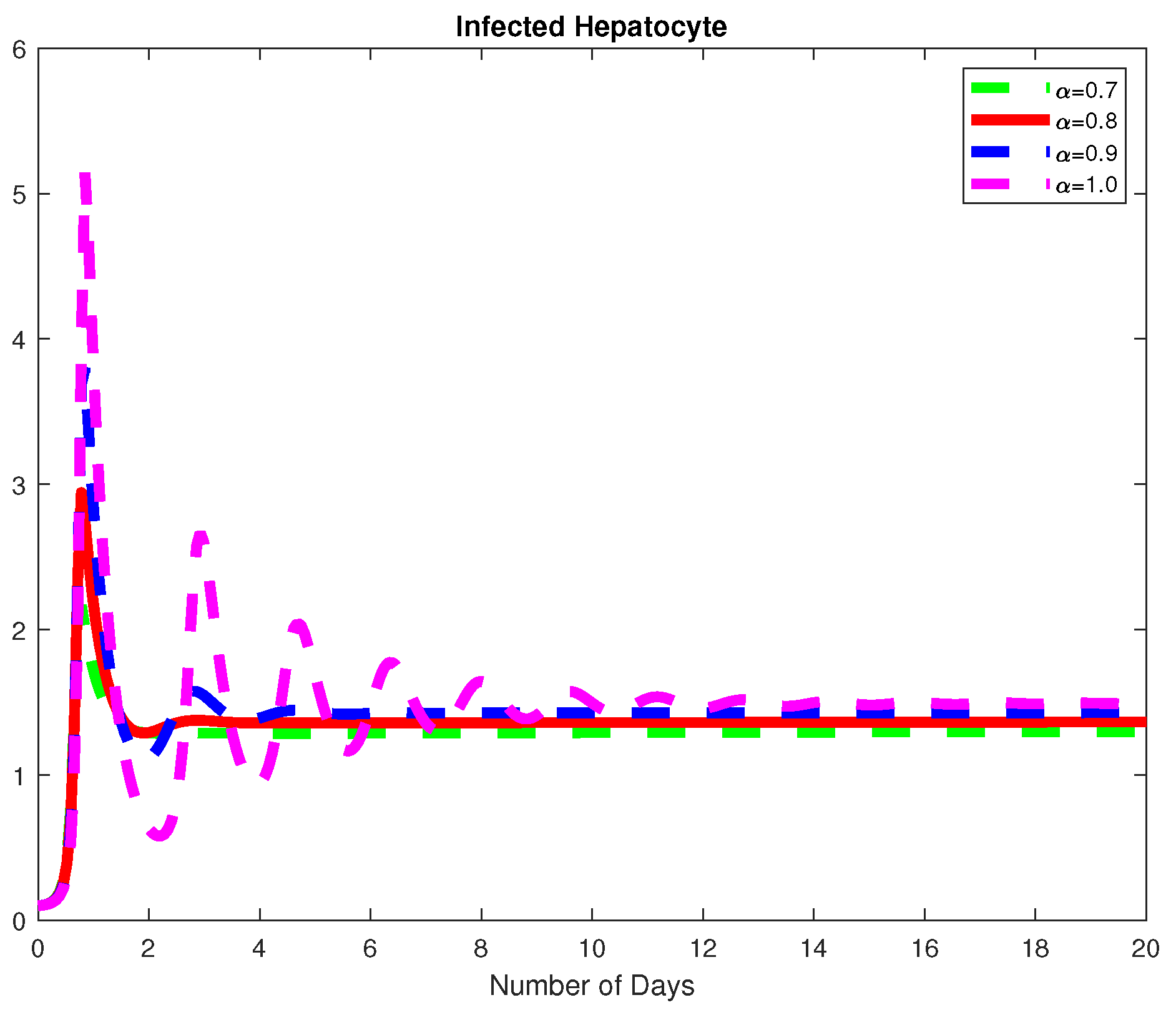
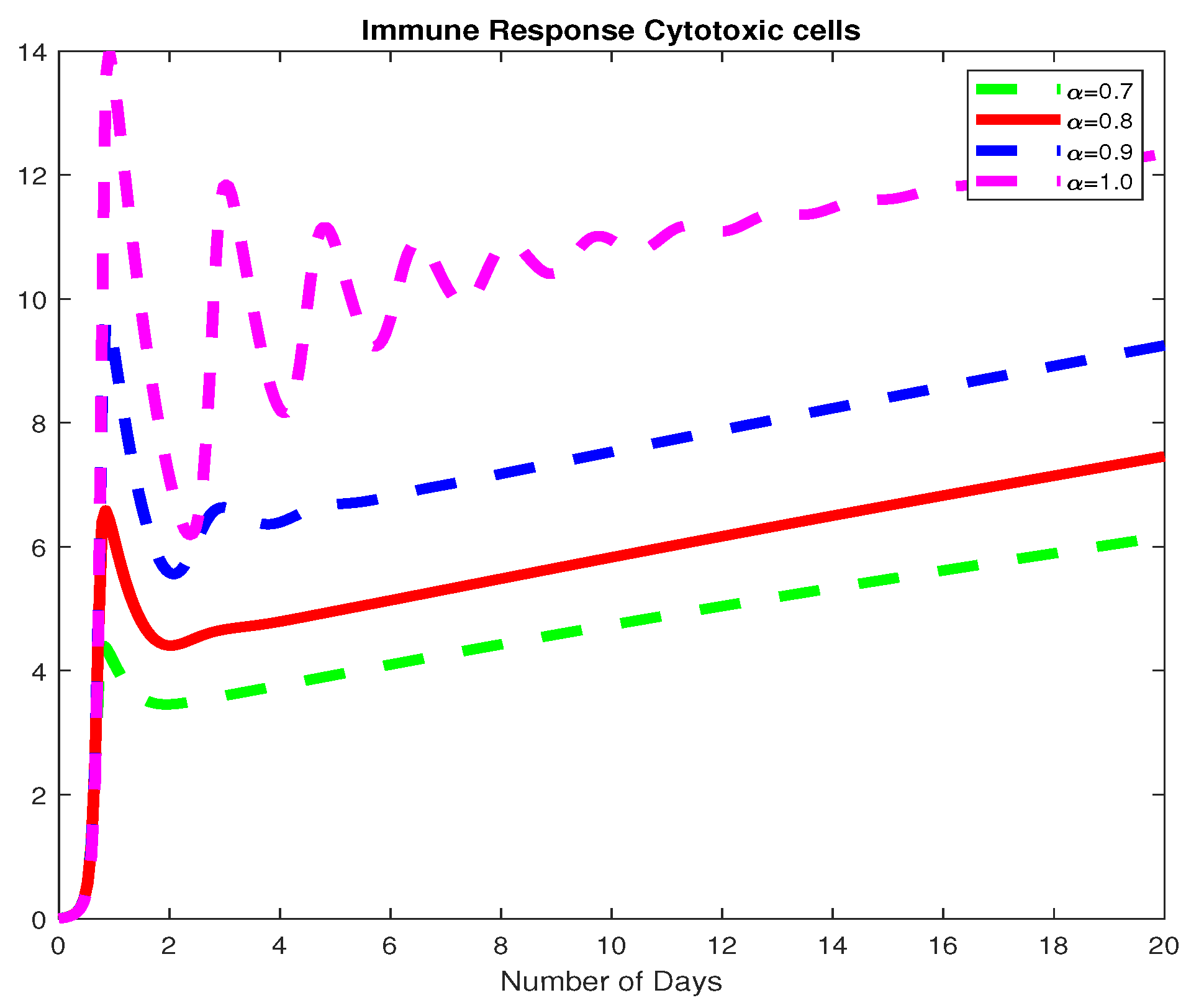
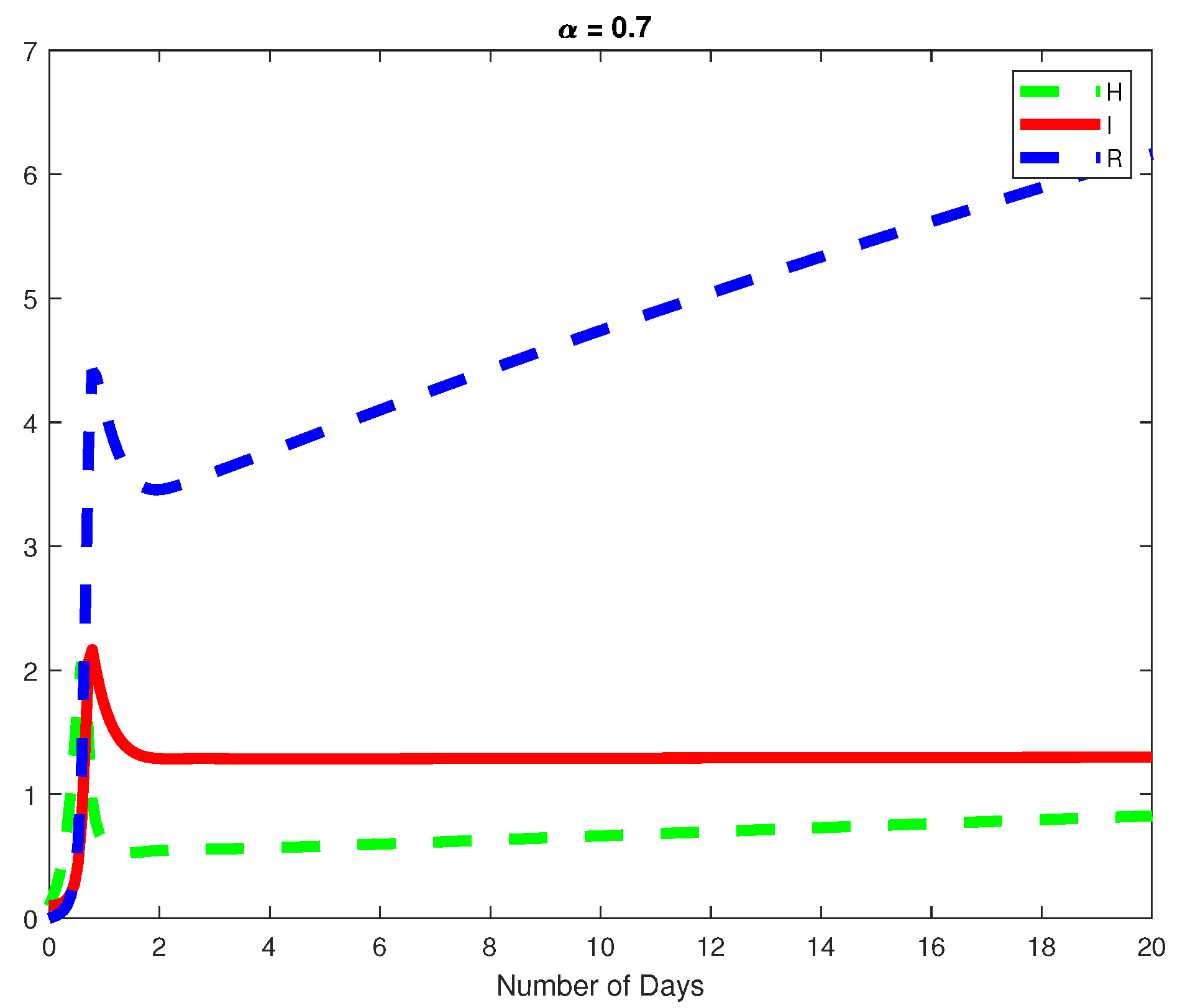
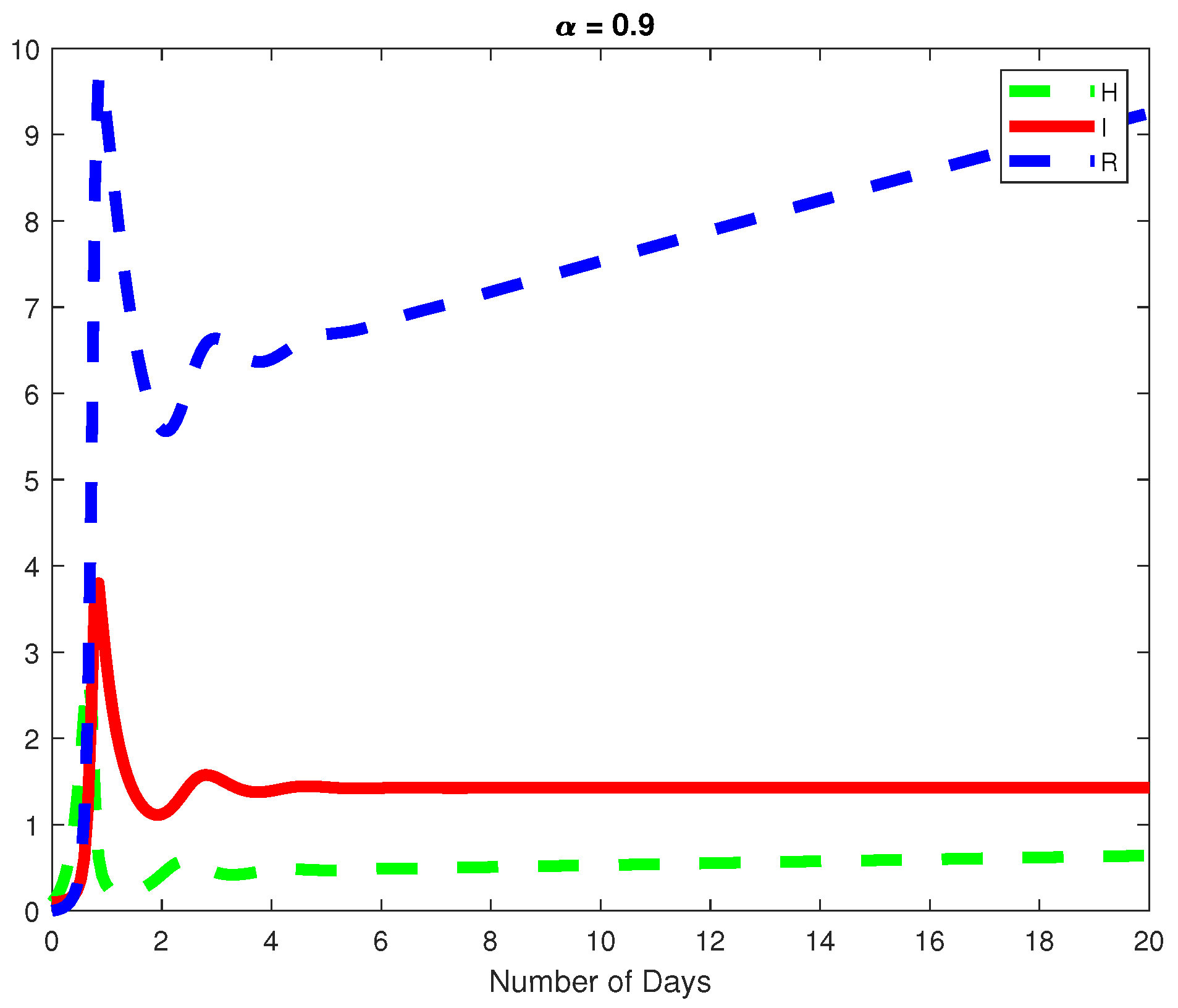
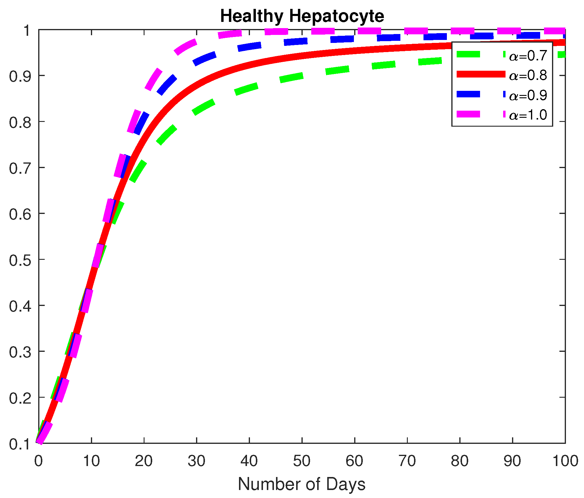
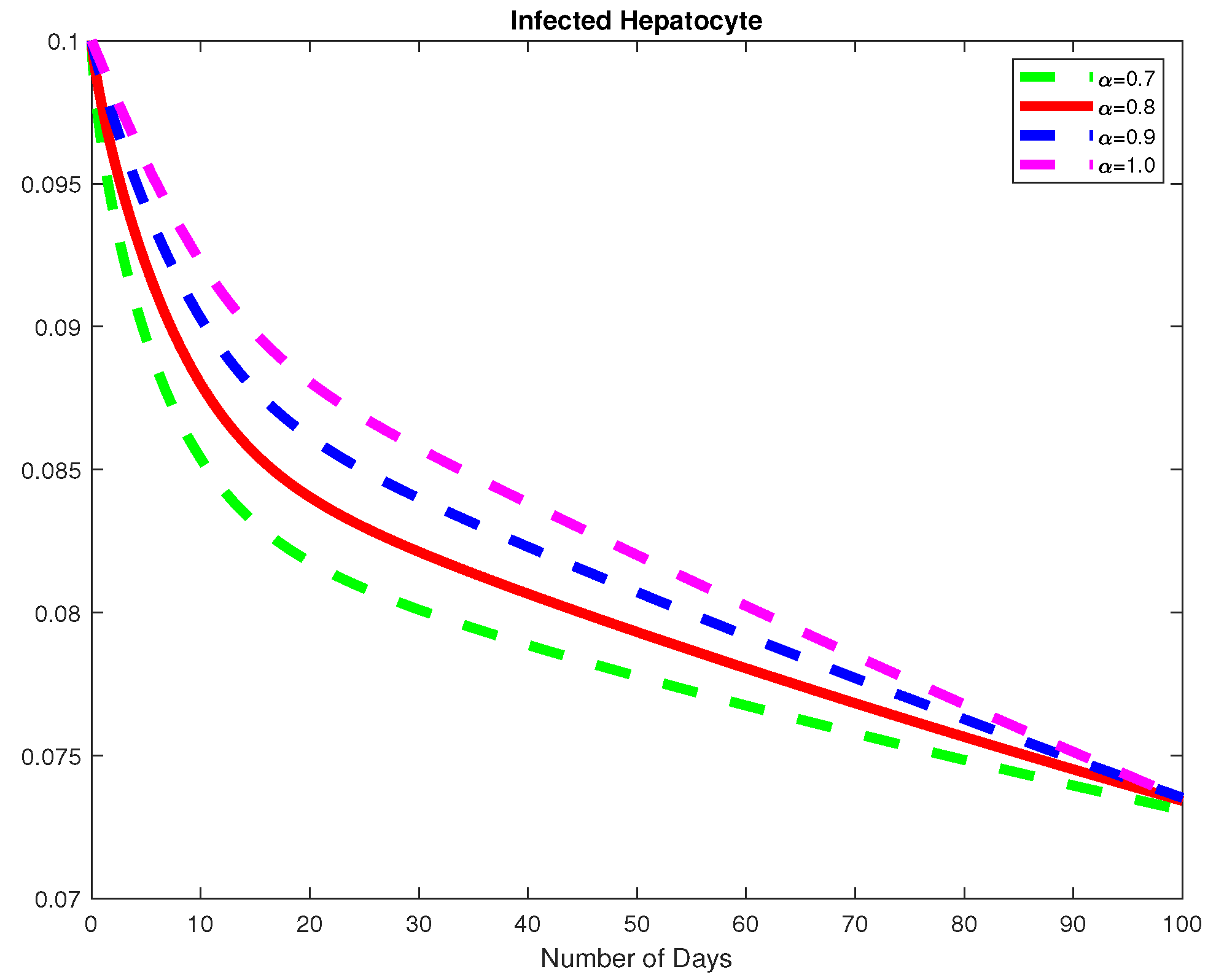
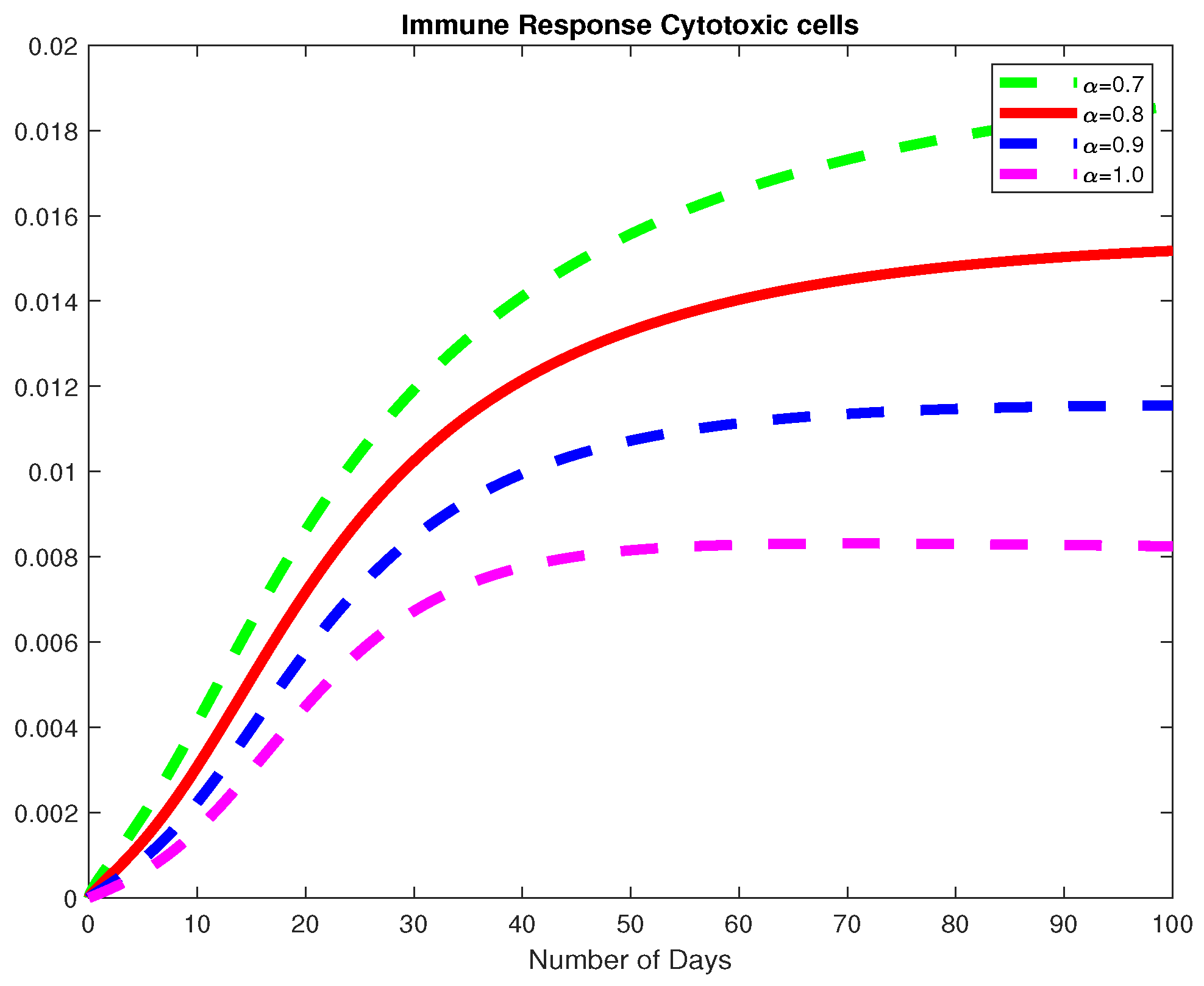
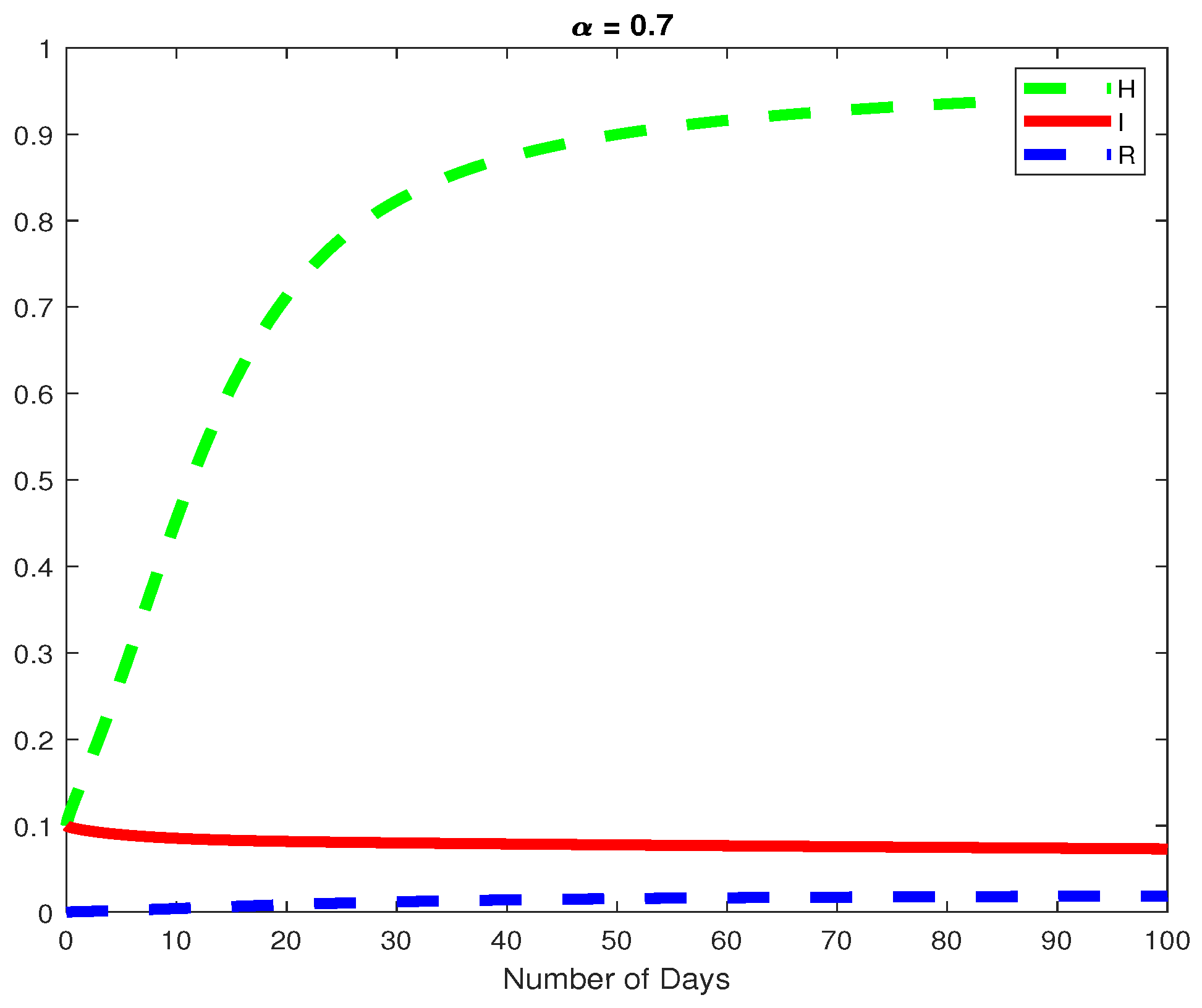
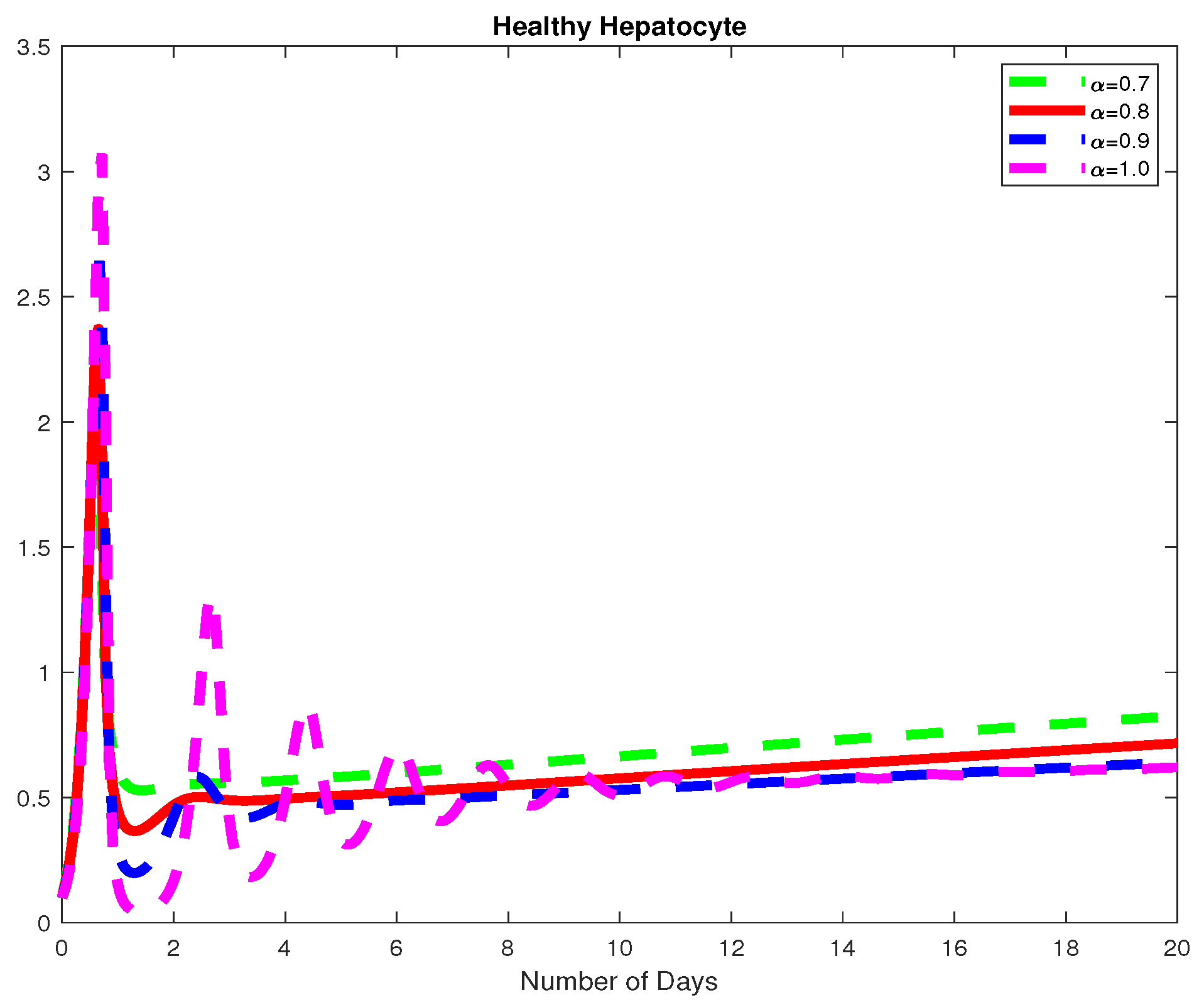
In this example, we assume parameter values as follows $\beta =4.14704,{\mu }_1=0.0693,$${\mu }_2=0.693,\tau =10,\sigma =1.35,r_1=6.2,r_2=0.02,c_1=0.2,c_2=0.037,K=2\times {10}^{11}.$ We consider the initial conditions $H_0=0.1,I_0=0.1,R_0=0$ with a time span of 0 to 20 days and varying values of the fractional order $\alpha$ are reported in Figure 1, Figure 2 and Figure 3. Finally in Figure 4 and Figure 5, we present the dynamics of the model for $\alpha =0.7$ and $\alpha =0.9.$ Here, we obtain a basic reporduction number ${\mathcal{R}}_0>1.$ This example demonstrates the case where the healthy hepatocytes are growing slower than the infected hepatocytes, which activates the growth of more immune response cytotoxic cells, as can be seen in Figure 3 and Figure 4.

Figure 1. The dynamics of the healthy hepatocytes, $H,$ for varying fractional order $\alpha$.

Figure 2. The dynamics of the Infected hepatocytes, $I,$ for varying fractional order $\alpha$.

Figure 3. The dynamics of the immune response cytotoxic cells, $R,$ for varying fractional order $\alpha$.

Figure 4. For the same fractional order, we plot the dynamics of the Healthy and Infected Hepatocyte as well as the Immune response cytotoxic cells for $\alpha =0.7$.

Figure 5. For the same fractional order, we plot the dynamics of the Healthy and Infected Hepatocyte as well as the Immune response cytotoxic cells for $\alpha =0.9$.

5.2. Example 2

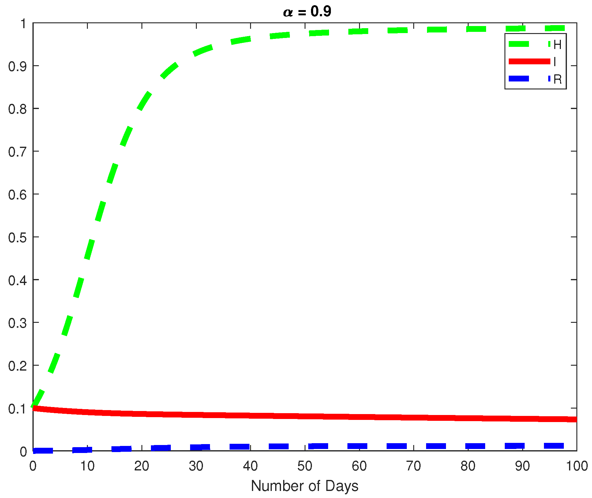
In this example, we consider the parameters values $r_1=0.2,K=1,\beta =0.3,$$c_1=0.02,{\mu }_1=0.01,\tau =0.0001,\sigma =0.001,r_2=0.01,c_2=1,{\mu }_2=0.02.$ Here, we demonstrate the case where ${\mathcal{R}}_0\le 1,$ which means that the virus will die out after a number of days, see Figure 6, Figure 7 and Figure 8. Again we see in Figure 9 and Figure 10, the dynamics of the model for varying parameters $\alpha =0.7$ and $\alpha =0.9.$ This example demonstrates the case where the healthy hepatocytes are growing faster than the infected hepatocytes. This activates a minimal growth of immune response cytotoxic cells, as can be seen in Figure 9 and Figure 10.

Figure 6. The dynamics of the healthy hepatocytes, $H,$ for varying fractional order $\alpha$.

Figure 7. The dynamics of the infected hepatocytes, $I,$ for varying fractional order $\alpha$.

Figure 8. The dynamics of the immune response cytotoxic cells, $R,$ for varying fractional order $\alpha$.

Figure 9. The dynamics of the Healthy $\left(H\right)$ and Infected $\left(I\right)$ Hepatocyte and the Immune resonse cytotoxic cells $\left(R\right)$ for $\alpha =0.7$.

Figure 10. The dynamics of the Healthy $\left(H\right)$ and Infected $\left(I\right)$ Hepatocyte and the Immune response cytotoxic cells $\left(R\right)$ for $\alpha =0.9$.

5.3. Example 3

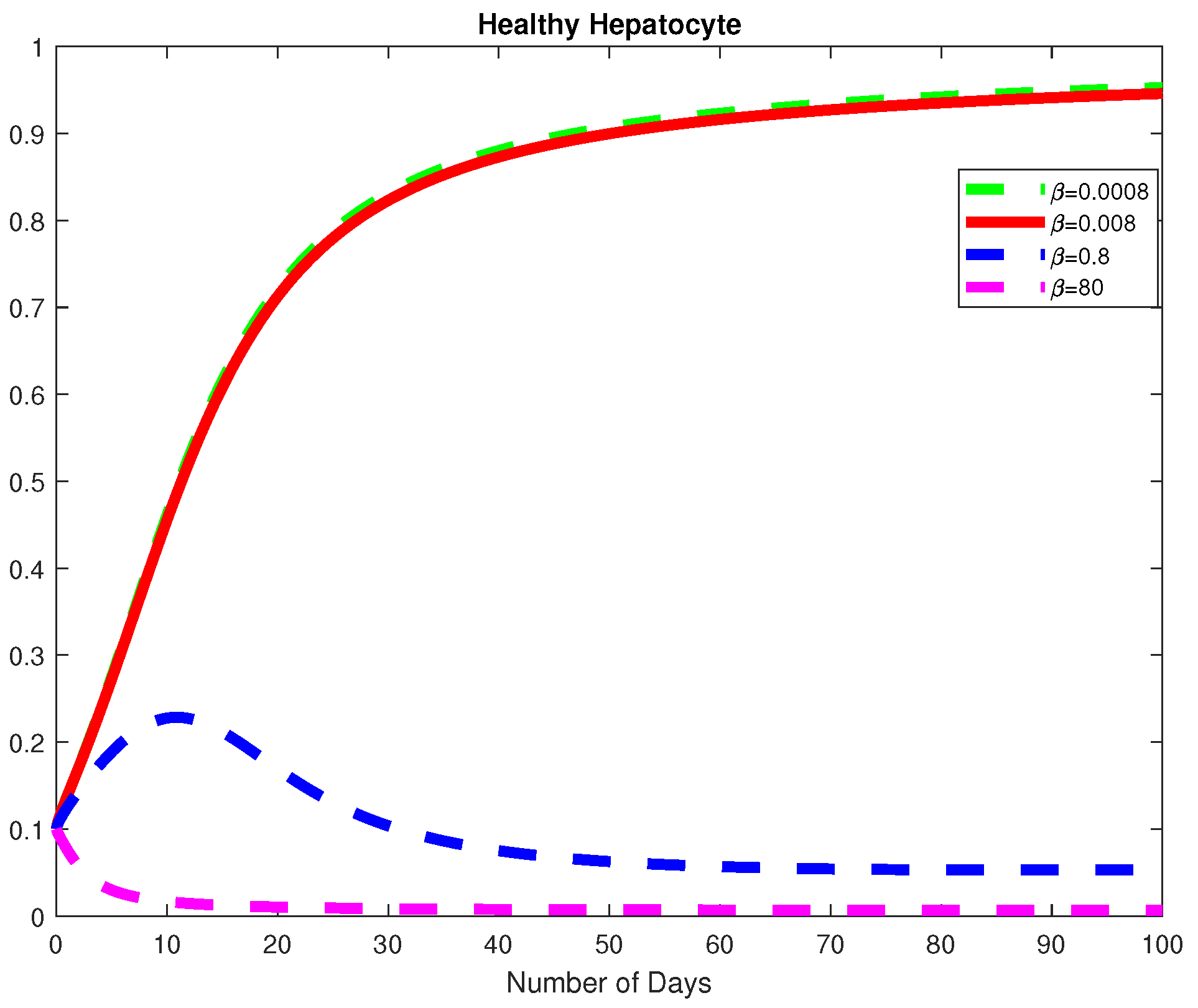
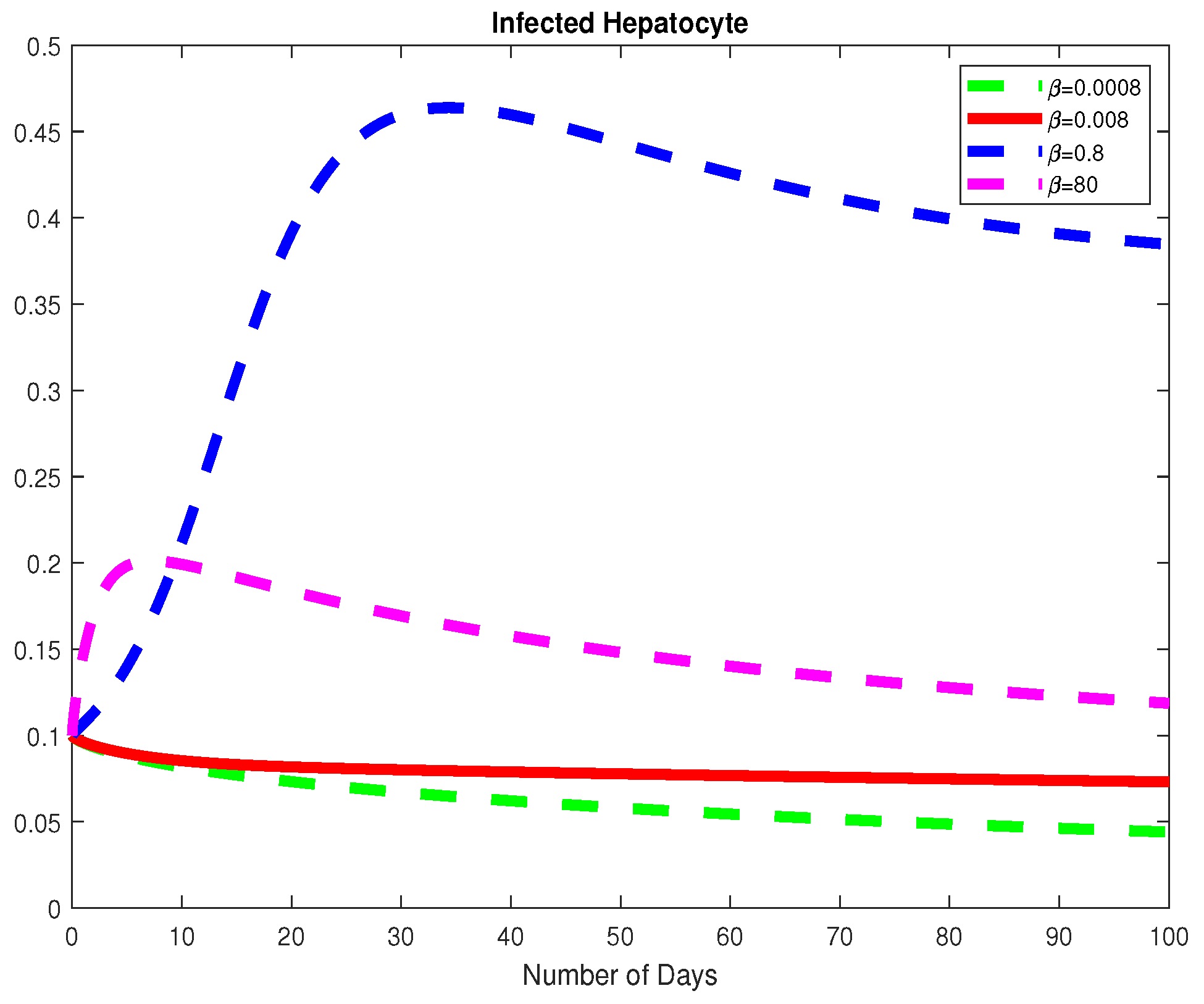
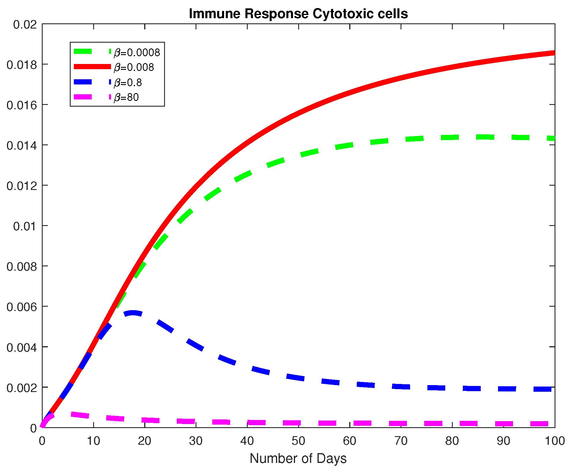
Next, we study the parameters $\beta$ and ${\mu }_1$ to understand the dynamics of the model with respect to the basic reproduction number, ${\mathcal{R}}_0.$ Using the parameter values from Example 2 at a fractional order of $\alpha =0.7,$ we choose varying values for $\beta .$ Here, we note that the basic viral reproduction number ${\mathcal{R}}_0<1,$ for $\beta =\{0.0008,0.008\}.$ Thus, if the infection rate of the normal cells is less than the natural death rate of the HB virus; then the HB virus will finally die out as depicted in Figure 11, Figure 12 and Figure 13. We also notice that, for $\beta <{\mu }_1,$ the Healthy Hepatocytes grow whiles the for $\beta >{\mu }_1,$ the Healthy Hepatocytes diminishes.

Figure 11. The dynamics of the Healthy Hepatocytes $\left(H\right)$ for varying values of $\beta$.

Figure 12. The dynamics of the Infected Hepatocytes $\left(I\right)$ for varying values of $\beta$.

Figure 13. The dynamics of the Immune Response Cytotoxic cells $\left(R\right)$ for varying values of $\beta$.

5.4. Example 4

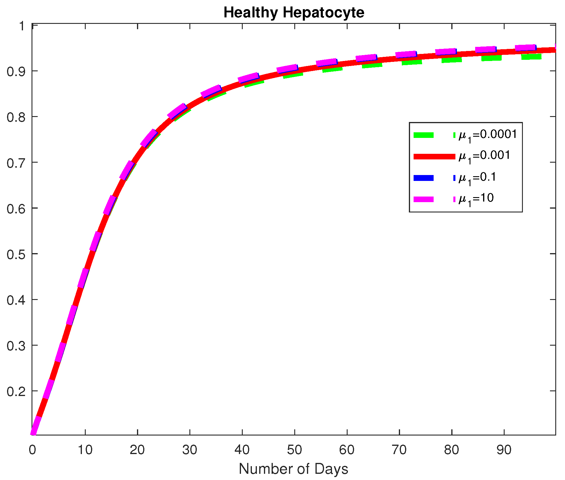
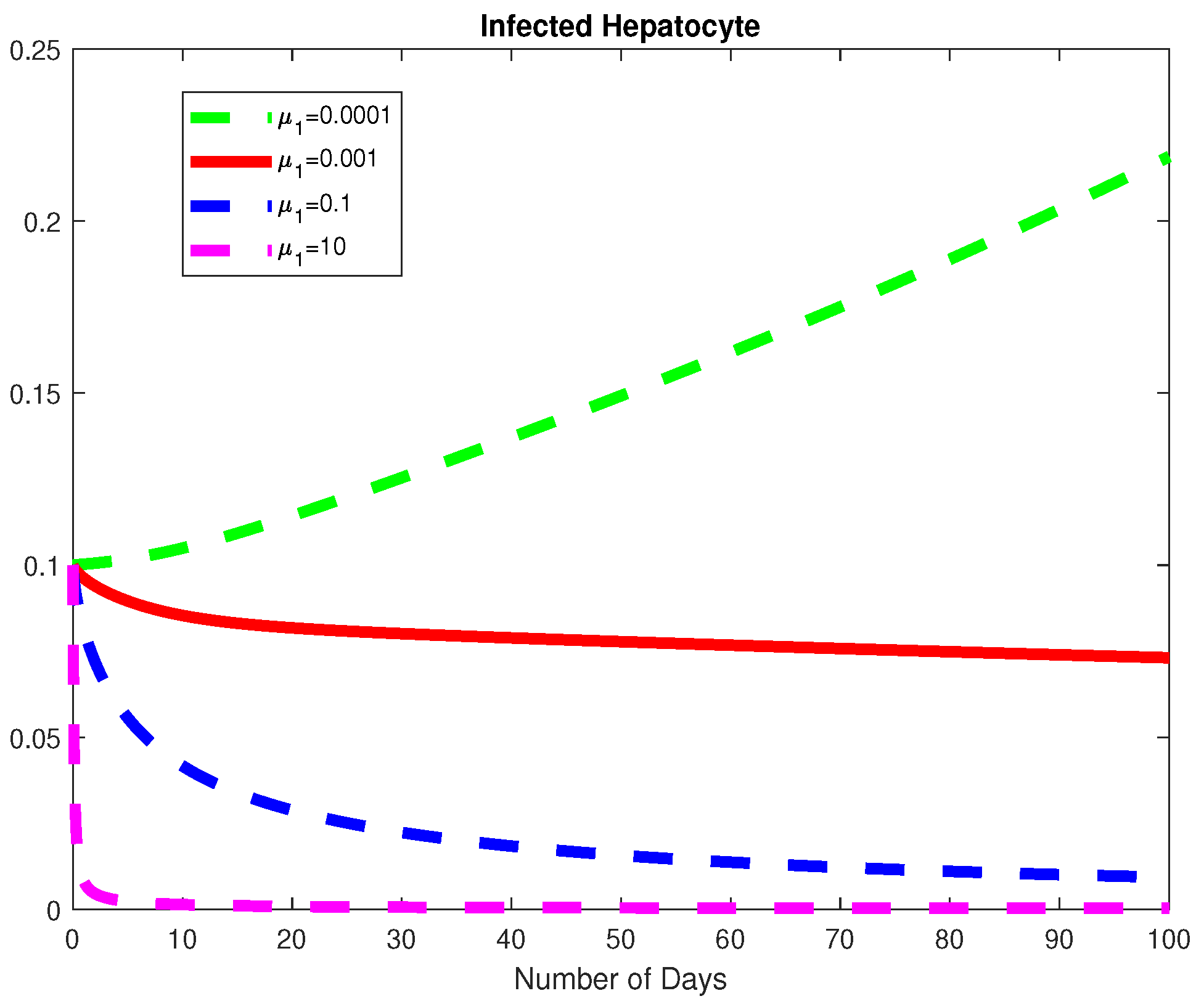
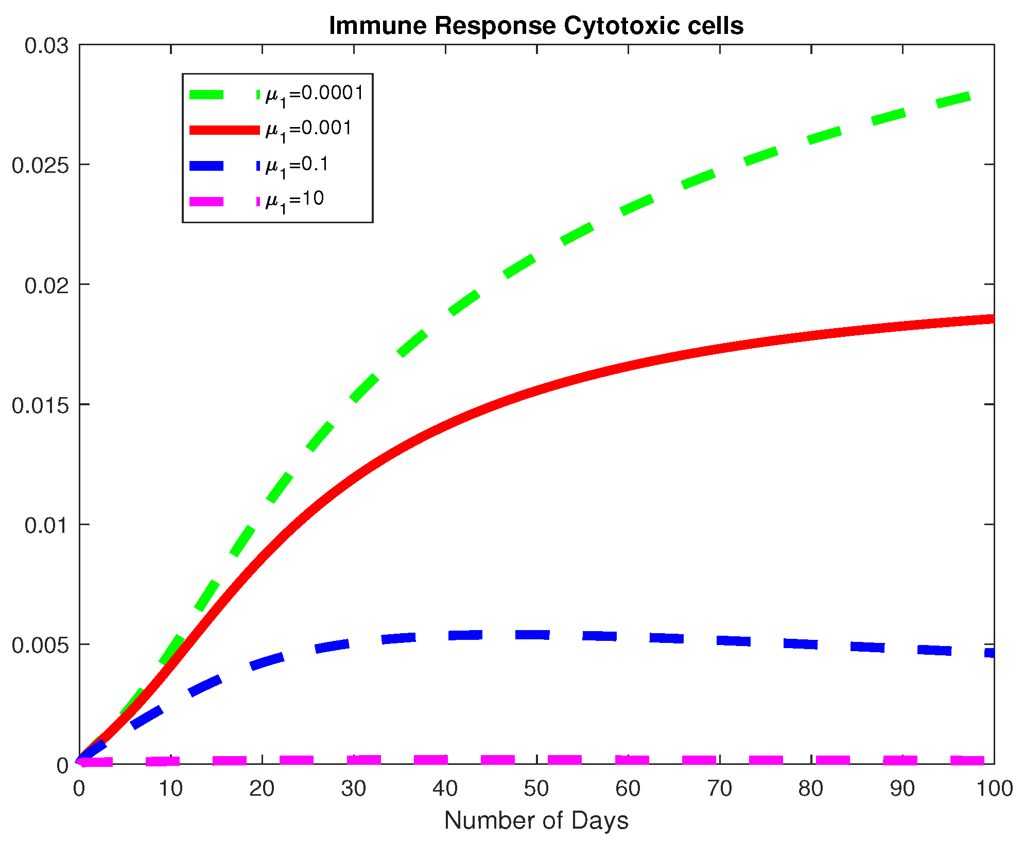
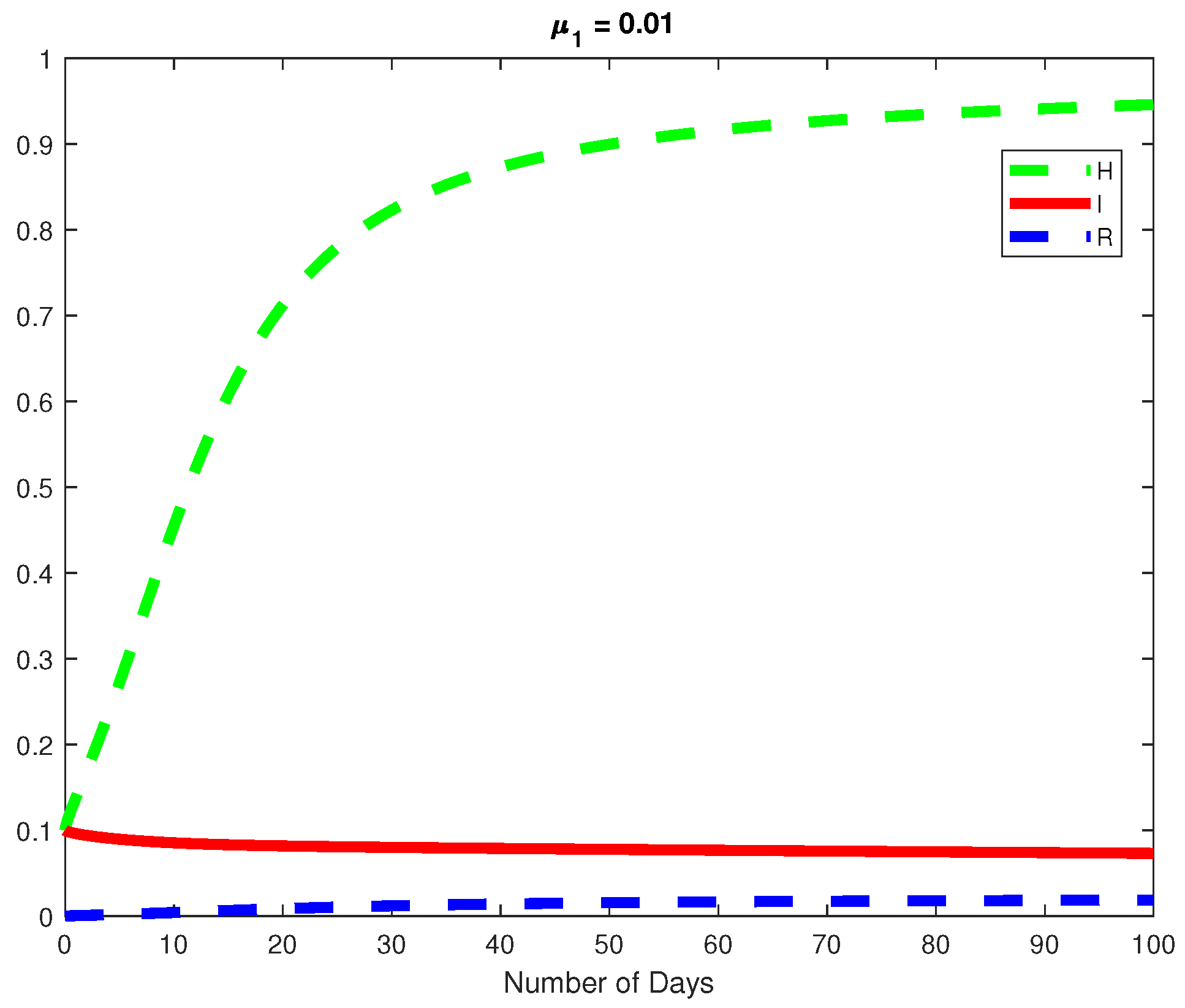
In this example, we consider all the parameter values in Example 2 except for ${\mu }_1$ for a fixed fractional order $\alpha =0.7.$ We used varying values of ${\mu }_1=\{0.0001,0.001,0.1,10\}.$ We obtained the basic viral reproduction number ${\mathcal{R}}_0<1$ for all the values except at ${\mu }_1=0.0001,$ which means that the virus will be removed whenever the natural death rate of the virus is less than the rate of infection of healthy hepatocytes, see Figure 14, Figure 15 and Figure 16. In Figure 17, we notice that when the Healthy Hepatocytes are high, the infected Hepatocytes are low and lead to a low amount of the immune response cytotoxic cells.

Figure 14. The dynamics of the Healthy Hepatocytes $\left(H\right)$ for varying values of ${\mu }_1$.

Figure 15. The dynamics of the Infected Hepatocytes $\left(I\right)$ for varying values of ${\mu }_1$.

Figure 16. The dynamics of the Immune response cytotoxic cells $\left(R\right)$ for varying values of ${\mu }_1$.

Figure 17. The dynamics of the model for ${\mu }_1=0.01$ at a fractional order of $\alpha =0.7$.

Analyzing the impact of K in the model, we realize that, in both endemic and disease-free states, a significant increase in the value of K does not change the state of stability, for instance, keeping all parameters constant in the case of endemic with ${\mu }_1=0.01$, when $K=10,{\mathcal{R}}_0=6>1$, and when $K=1000,{\mathcal{R}}_0=600>1$. we also analyzed $\beta$, which affects the rate at which Healthy hepatocytes become infected; thus, an increase in $\beta$ always causes the infected hepatocytes to increase, indicating a positive relationship between $\beta$ and I. An increase in $\beta$ in an endemic condition indicates that the virus will eventually affect all the healthy hepatocytes, and once there are no healthy hepatocytes left to rely on, the virus will eventually go extinct see (Figure 10). Taking $\alpha =1$, when ${\mu }_1=0.01$ and $\beta =0.3$, ${\mathcal{R}}_0=30$. similarly when $\beta =0.1$, ${\mathcal{R}}_0=10$. The maximum value $\beta$ can take in the endemic case is $1.2$ and a minimum value of $0.1$. In the case of disease free when ${\mu }_1=0.5$, $\beta$ takes values $0<\beta <0.5$. Thus, when $\beta =0.3$, ${\mathcal{R}}_0=0.6<1$ and when $\beta =0.4$, ${\mathcal{R}}_0=0.8<1$.

6. Conclusions

We presented the theoretical and numerical simulations for Caputo fractional order model for Hepatitis B cellular viral infection. We presented the existence and uniqueness as well as the boundedness of the model. We showed that the virus-free equilibrium (VFE) is locally asymptotically stable when ${\mathcal{R}}_0\le 1$ else is unstable, i.e., replicating and becomes persistent in the liver. By means of Routh–Hurwitz, we established local stability. Using Ulam–Hyers stability, we showed that the fractional model is globally asymptotically stable. Subsequently, we presented the global stability results for the virus-free and endemic equilibrium points. Finally, using a predictor–corrector iterative scheme, several numerical simulations were presented for different fractional orders of the derivative, which corresponds to the analytical results predicted.

References

1. Rehermann, B.; Ferrari, C.; Pasquinelli, C.; Chisari, F.V. The hepatitis B virus persists for decades after patients’ recovery from acute viral hepatitis despite active maintenance of a cytotoxic T–lymphocyte response. Nat. Med. 1996, 2, 1104–1108. [Google Scholar]
2. Wieland, S.F.; Spangenberg, H.C.; Thimme, R.; Purcell, R.H.; Chisari, F.V. Expansion and contraction of the hepatitis B virus transcriptional template in infected chimpanzees. Proc. Natl. Acad. Sci. USA 2004, 101, 2129–2134. [Google Scholar] [CrossRef]
3. Guidotti, L.G.; Ishikawa, T.; Hobbs, M.V.; Matzke, B.; Schreiber, R.; Chisari, F.V. Intracellular inactivation of the hepatitis B virus by cytotoxic T lymphocytes. Immunity 1996, 4, 25–36. [Google Scholar] [CrossRef] [PubMed]
4. Reuter, T.Q.; Gomes-Gouvea, M.; Chuffi, S.; Duque, U.H.; Carvalho, J.A.; Perini, W.; Queiroz, M.M.; Segal, I.M.; Azevedo, R.S.; Pinho, J.R.R. Hepatitis B virus genotypes and subgenotypes and the natural history and epidemiology of hepatitis B. Ann. Hepatol. 2022, 27, 100574. [Google Scholar] [PubMed]
5. Khan, T.; Jung, I.H.; Khan, A.; Zaman, G. Classification and sensitivity analysis of the transmission dynamic of hepatitis B. Theor. Biol. Med. Model. 2017, 14, 1–17. [Google Scholar]
6. Bachraoui, M.; Ichou, M.A.; Hattaf, K.; Yousfi, N. Spatiotemporal dynamics of a fractional model for hepatitis B virus infection with cellular immunity. Math. Model. Nat. Phenom. 2021, 16, 5. [Google Scholar]
7. Yang, X.; Su, Y.; Yang, L.; Zhuo, X. Global analysis and simulation of a fractional order HBV immune model. Chaos Solitons Fractals 2022, 154, 111648. [Google Scholar] [CrossRef]
8. Khatun, Z.; Islam, M.S.; Ghosh, U. Mathematical modeling of hepatitis B virus infection incorporating immune responses. Sensors Int. 2020, 1, 100017. [Google Scholar]
9. Fatehi Chenar, F.; Kyrychko, Y.; Blyuss, K. Mathematical model of immune response to hepatitis B. J. Theor. Biol. 2018, 447, 98–110. [Google Scholar] [CrossRef] [PubMed]
10. Kilbas, A.A.; Srivastava, H.M.; Trujillo, J.J. Theory and Applications of Fractional Differential Equations; Elsevier: Amsterdam, The Netherlands, 2006; Volume 204. [Google Scholar]
11. Podlubny, I. Fractional Differential Equations: An Introduction to Fractional Derivatives, Fractional Differential Equations, to Methods of Their Solution and Some of Their Applications; Academic Press: San Diego, CA, USA, 1999. [Google Scholar]
12. Komarova, N.L.; Barnes, E.; Klenerman, P.; Wodarz, D. Boosting immunity by antiviral drug therapy: A simple relationship among timing, efficacy, and success. Proc. Natl. Acad. Sci. USA 2003, 100, 1855–1860. [Google Scholar] [PubMed]
13. Eikenberry, S. A tumor cord model for doxorubicin delivery and dose optimization in solid tumors. Theor. Biol. Med Model. 2009, 6, 1–20. [Google Scholar] [CrossRef] [PubMed]
14. Ribeiro, R.M.; Perelson, A.S. Hepatitis B virus viral dynamics: Effects of drug dose and baseline alanine aminotransferase. J. Hepatol. 2002, 37, 277–279. [Google Scholar] [PubMed]
15. Diethelm, K. A fractional calculus based model for the simulation of an outbreak of dengue fever. Nonlinear Dyn. 2013, 71, 613–619. [Google Scholar] [CrossRef]
16. Sardar, T.; Rana, S.; Bhattacharya, S.; Al-Khaled, K.; Chattopadhyay, J. A generic model for a single strain mosquito-transmitted disease with memory on the host and the vector. Math. Biosci. 2015, 263, 18–36. [Google Scholar] [CrossRef] [PubMed]
17. Lin, W. Global existence theory and chaos control of fractional differential equations. J. Math. Anal. Appl. 2007, 332, 709–726. [Google Scholar] [CrossRef]
18. Li, M.Y. An Introduction to Mathematical Modeling of Infectious Diseases; Springer: Berlin/Heidelberg, Germany, 2018; Volume 2. [Google Scholar]
19. Harianto, J. Local stability analysis of an SVIR epidemic model. CAUCHY 2017, 5, 20–28. [Google Scholar] [CrossRef]
20. Adda, P.; Bichara, D. Global stability for SIR and SIRS models with differential mortality. arXiv 2011, arXiv:1112.2662. [Google Scholar]
21. Diethelm, K.; Ford, N.J.; Freed, A.D. Detailed error analysis for a fractional Adams method. Numer. Algorithms 2004, 36, 31–52. [Google Scholar]
22. Diethelm, K.; Ford, N.J.; Freed, A.D. A predictor-corrector approach for the numerical solution of fractional differential equations. Nonlinear Dyn. 2002, 29, 3–22. [Google Scholar] [CrossRef]