
The Binomial–Natural Discrete Lindley Distribution: Properties and Application to Count Data


Abstract
:1. Introduction
2. Natural Discrete Lindley Distribution
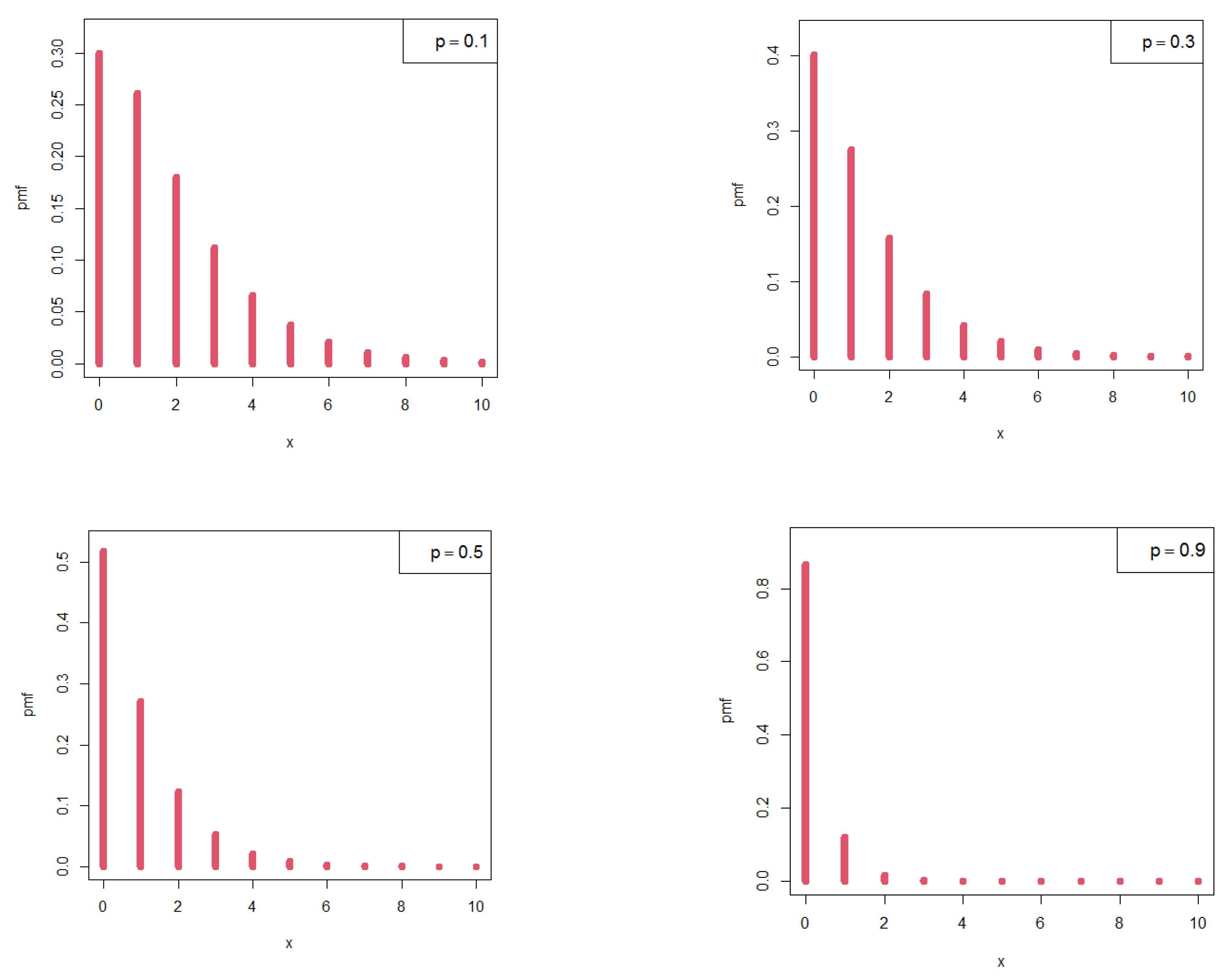
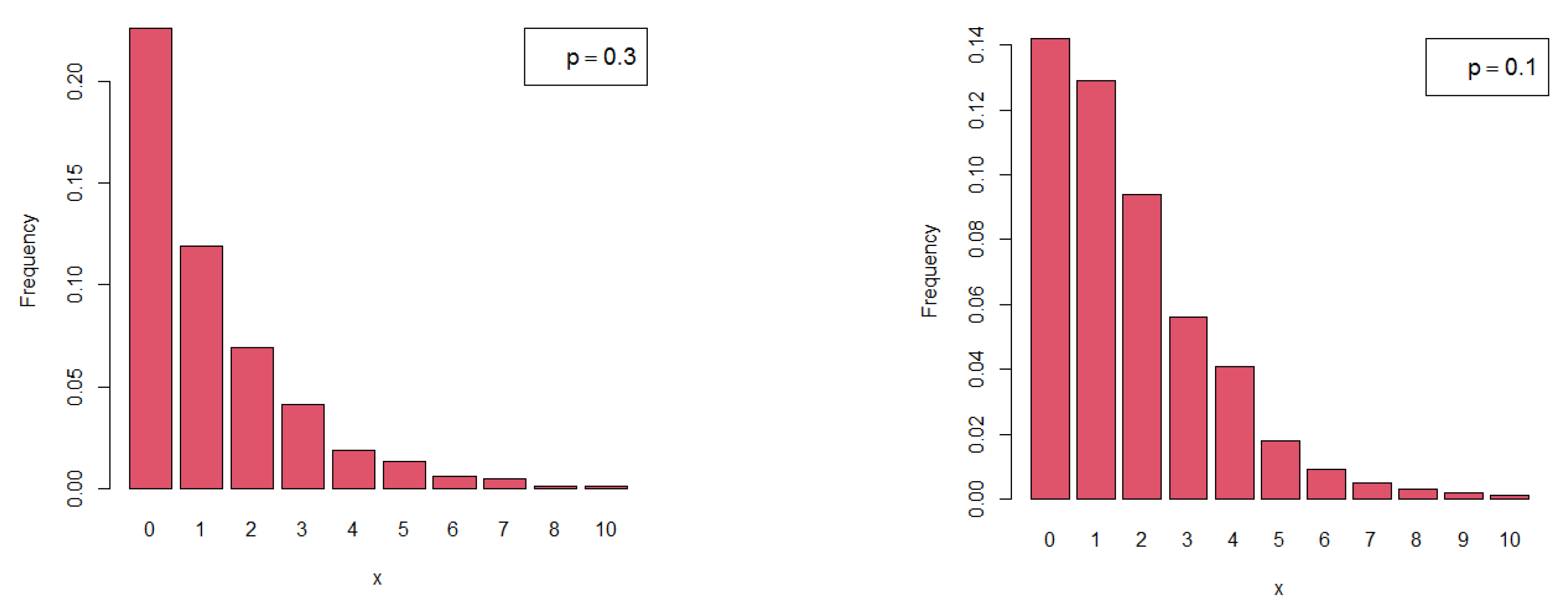
2.1. The Proposed Discrete Analog
2.2. Statistical Properties of the BNDL Distribution
2.2.1. Moment-Generating Function
2.2.2. Probability-Generating Function
2.2.3. Non-Central Moments and Variance
2.2.4. Central Moments
2.2.5. Skewness and Kurtosis
2.2.6. Index of Dispersion
2.2.7. Log-Concavity
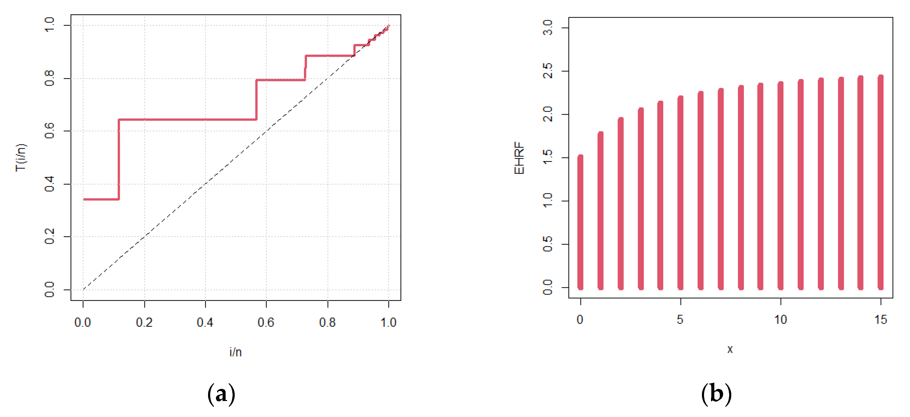
2.3. Reliability Properties of the BNDL Distribution
2.3.1. Survival Function
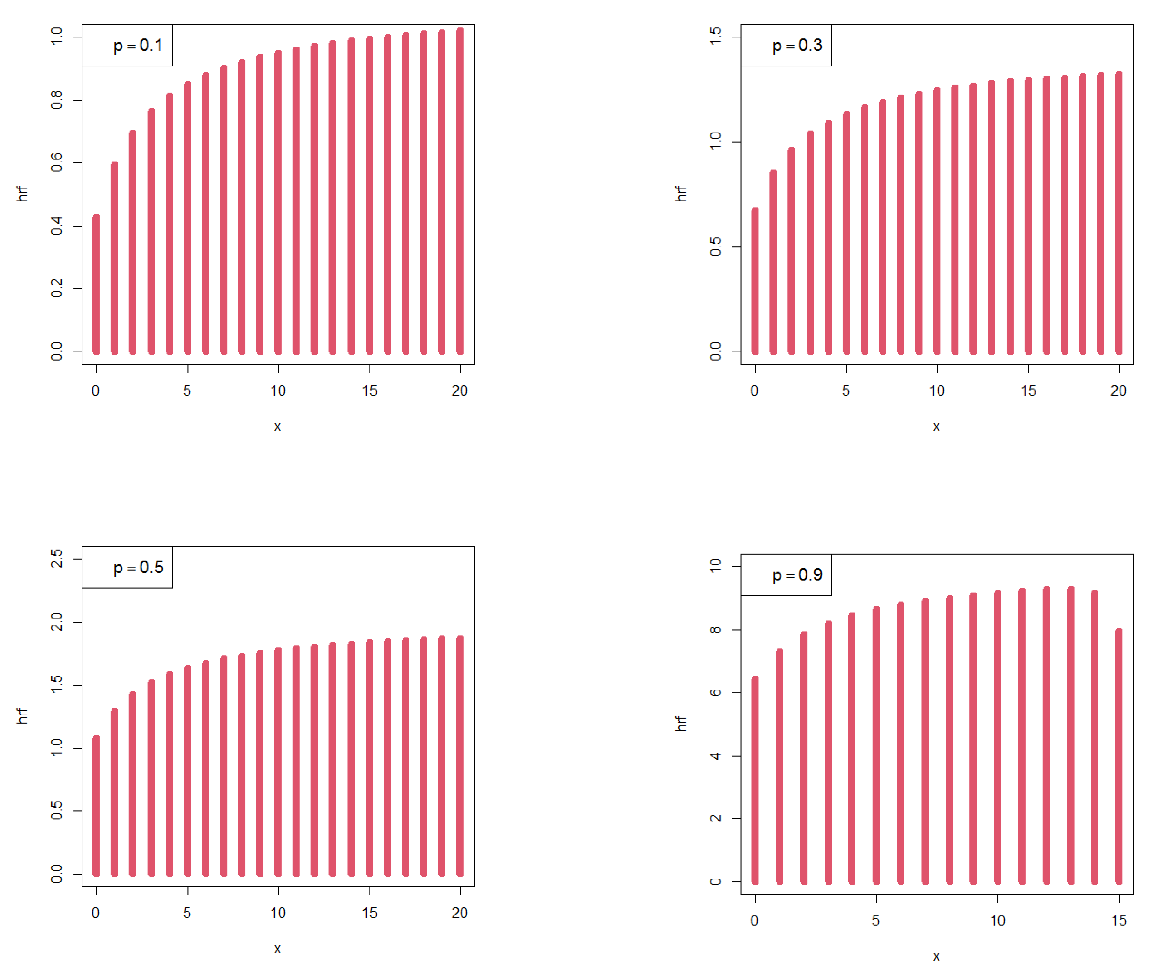
2.3.2. Hazard Rate and Mean Residual Life Functions
- IFR (increasing failure rate).
- IFRA(increasing failure rate average).
- NBU (new better than used).
- NBUE(new better than used in expectation).
- DMRL (decreasing mean residual lifetime).
2.4. Stochastic Orderings
- Usual stochastic order, denoted by , if , for all .
- Hazard rate order, denoted by , if , for all .
- Reversed hazard rate order, denoted by , if decreases in .
- Mean residual life order, denoted by , if , for all x.
- Likelihood ratio order, denoted by , if decreases in .
2.5. Entropy
3. Estimation and Simulation
3.1. Method of Maximum Likelihood Estimation
3.2. Method of Moments Estimation
3.3. Method of Proportions Estimation
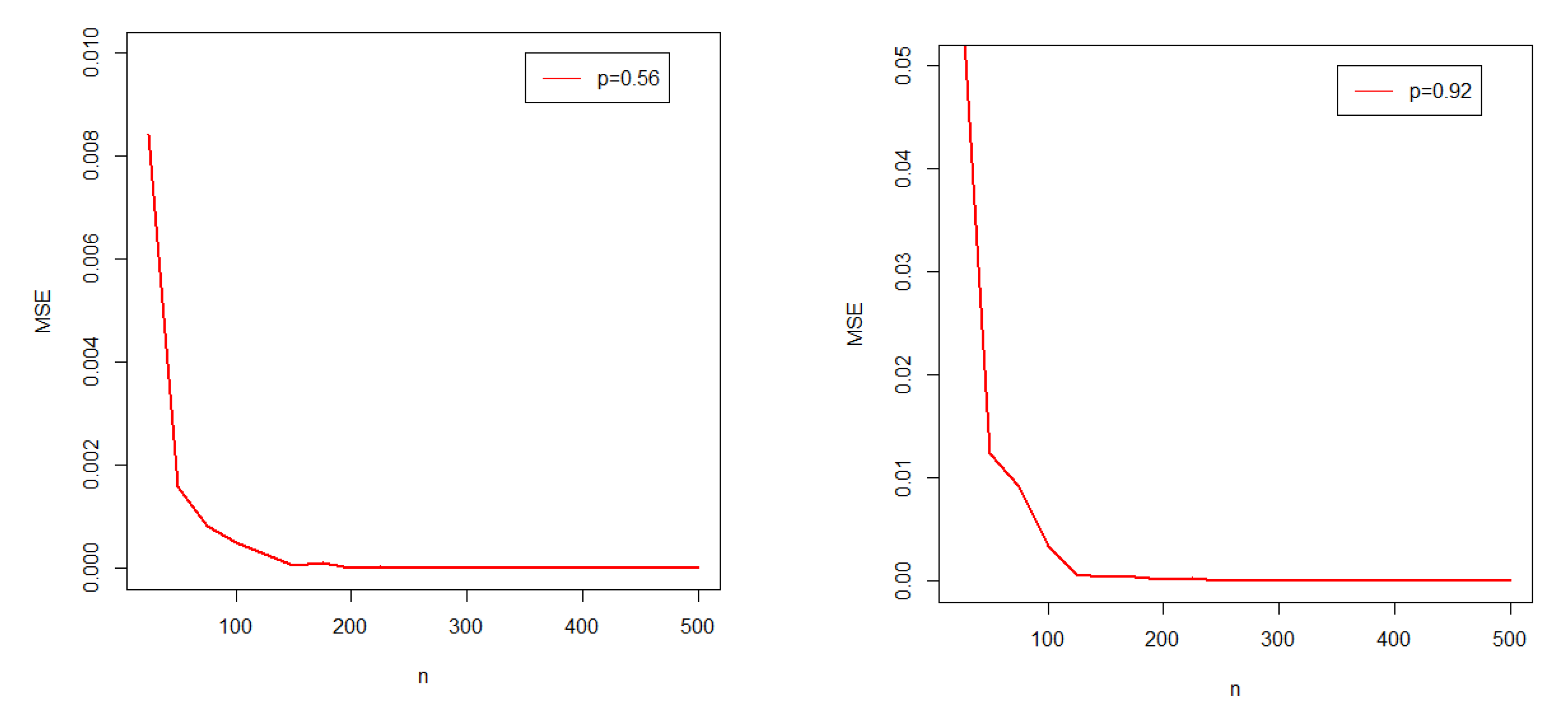
3.4. Simulation Study
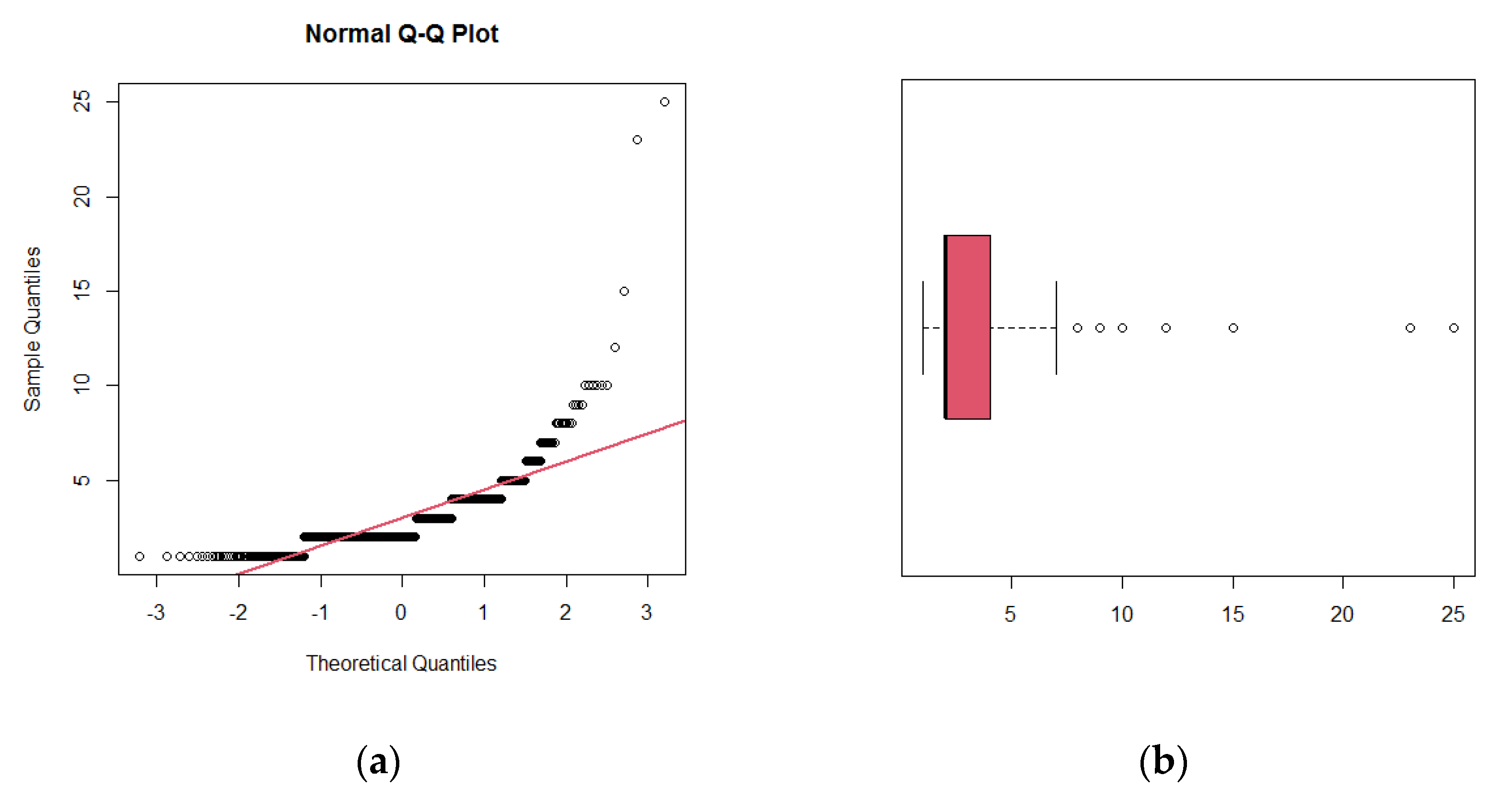
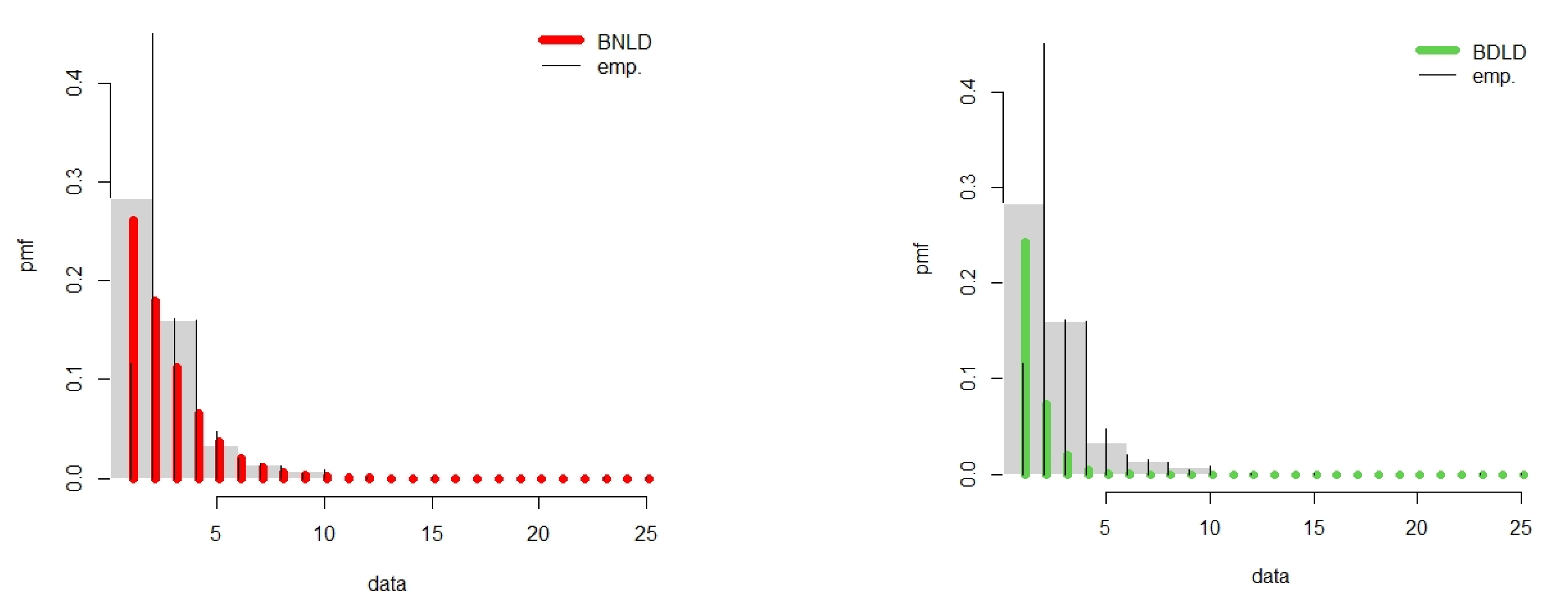
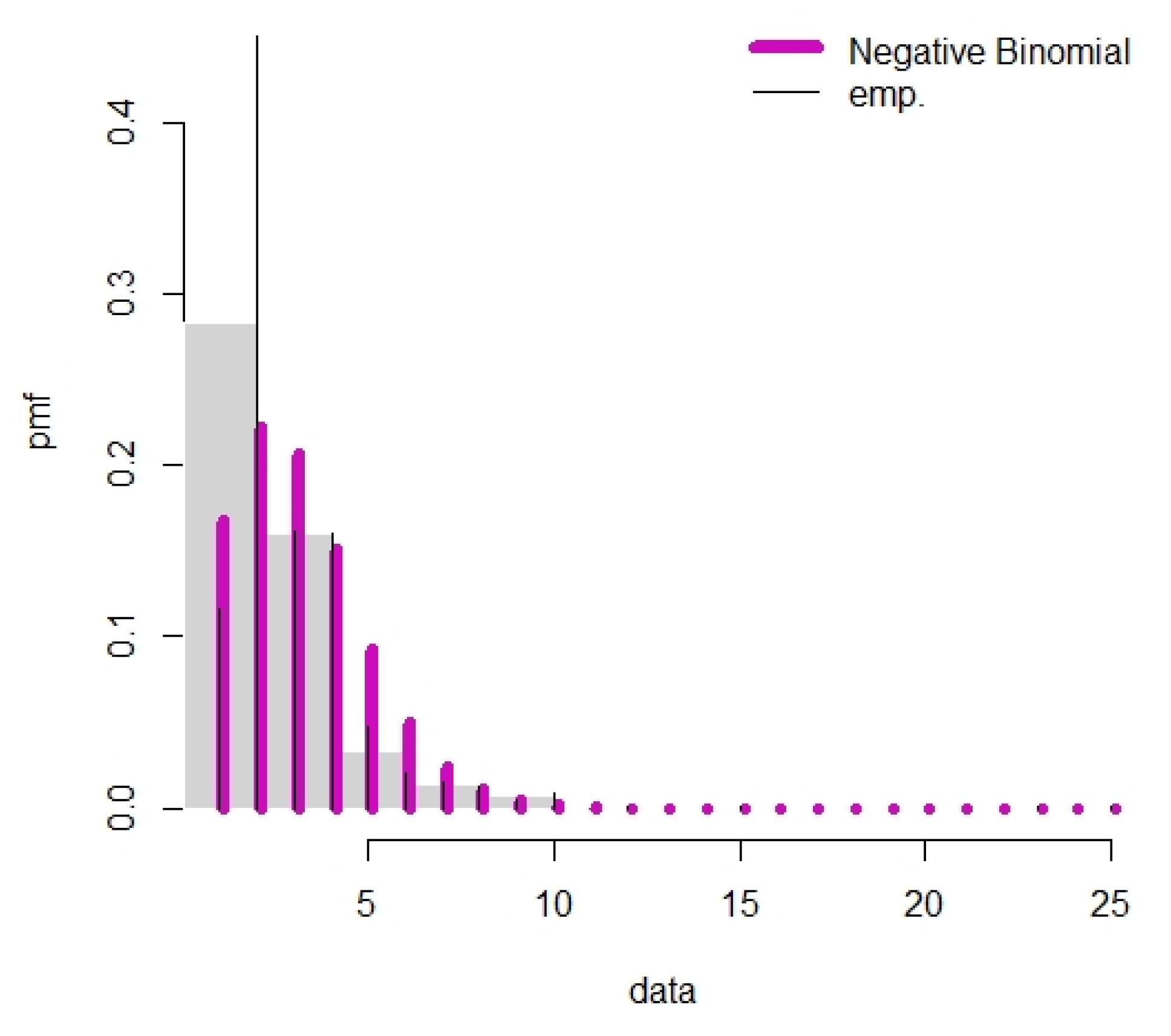
4. Applications to Count Data
| x | 1 | 2 | 3 | 4 | 5 | 6 | 7 | 8 | 9 | 10 and above |
| f | 86 | 235 | 120 | 119 | 35 | 15 | 11 | 9 | 4 | 10 |
5. Concluding Remarks
Author Contributions
Funding
Conflicts of Interest
References
- Aryuyuen, S.; Bodhisuwan, W.; Volodin, A. Discrete Generalized Odd Lindley—Weibull Distribution with Applications. Lobachevskii J. Math. 2020, 41, 945–955. [Google Scholar] [CrossRef]
- Chakraborty, S. A New Discrete Distribution Related to Generalized Gamma Distribution and Its Properties. Commun. Stat. Theory Methods 2015, 44, 1691–1705. [Google Scholar] [CrossRef]
- Chakraborty, S.; Chakravarty, D. Discrete Gamma Distributions: Properties and Parameter Estimations. Commun. Stat. Theory Methods 2012, 41, 3301–3324. [Google Scholar] [CrossRef]
- Chakraborty, S.; Dhrubajyoti, C. A Discrete Gumbel Distribution. arXiv 2014. Available online: https://arxiv.org/abs/1410.7568 (accessed on 8 June 2022).
- El-Morshedy, M.; Eliwa, M.S.; Nagy, H. A New Two-Parameter Exponentiated Discrete Lindley Distribution: Properties, Estimation and Applications. J. Appl. Stat. 2018, 47, 354–375. [Google Scholar] [CrossRef]
- Gómez-Déniz, E.; Calderín-Ojeda, E. The Discrete Lindley Distribution: Properties and Applications. J. Stat. Comput. Simul. 2011, 81, 1405–1416. [Google Scholar] [CrossRef]
- Hu, Y.; Peng, X.; Li, T.; Guo, H. On the Poisson Approximation to Photon Distribution for Faint Lasers. Phys. Lett. A 2007, 367, 173–176. [Google Scholar] [CrossRef] [Green Version]
- Shaked, M.; Shanthikumar, J.G. Stochastic Orders; Springer: New York, NY, USA, 2007. [Google Scholar] [CrossRef]
- Nekoukhou, V.; Alamatsaz, M.H.; Bidram, H. Discrete Generalized Exponential Distribution of a Second Type. Statistics 2013, 47, 876–887. [Google Scholar] [CrossRef]
- Para, B.A.; Jan, T.R. Discrete Generalized Weibull Distribution: Properties and Applications in Medical Sciences. Pak. J. Stat. 2017, 33, 337–354. [Google Scholar]
- Roy, D. The Discrete Normal Distribution. Commun. Stat.-Theory Methods 2003, 32, 1871–1883. [Google Scholar] [CrossRef]
- Afify, A.Z.; Elmorshedy, M.; Eliwa, M.S. A New Skewed Discrete Model: Properties, Inference, and Applications. Pak. J. Stat. Oper. Res. 2021, 17, 799–816. [Google Scholar] [CrossRef]
- Déniz, E.G. A New Discrete Distribution: Properties and Applications in Medical Care. J. Appl. Stat. 2013, 40, 2760–2770. [Google Scholar] [CrossRef]
- Akdoğan, Y.; Kuş, C.; Asgharzadeh, A.; Kinaci, I.; Sharafi, F. Uniform-Geometric Distribution. J. Stat. Comput. Simul. 2016, 86, 1754–1770. [Google Scholar] [CrossRef]
- Kuş, C.; Akdoğan, Y.; Asgharzadeh, A.; Kınacı, I.; Karakaya, K. Binomial-Discrete Lindley Distribution. Commun. Fac. Sci. Univ. Ank. Ser. A1 Math. Stat. 2019, 68, 401–411. [Google Scholar] [CrossRef]
- Al-Babtain, A.A.; Ahmed, A.H.N.; Afify, A.Z. A New Discrete Analog of the Continuous Lindley Distribution, with Reliability Applications. Entropy 2020, 22, 603. [Google Scholar] [CrossRef]
- Yalcin, F.; Simsek, Y. Formulas for characteristic function and moment generating functions of beta type distribution. Rev. Real Acad. Cienc. Exactas Físicas Y Naturales. Ser. A Matemáticas 2022, 116, 86. [Google Scholar] [CrossRef]
- Yalcin, F.; Simsek, Y. Anew class of symmetric beta type distributions constructed by means of symmetric Bernstein type basis functions. Symmetry 2020, 12, 779. [Google Scholar] [CrossRef]
- Simsek, B. Formulas derived from moment generating functions and Bernstein polynomials. Appl. Anal. Discret. Math. 2019, 13, 839–848. [Google Scholar] [CrossRef] [Green Version]
- Keilson, J.; Gerber, H. Some Results for Discrete Unimodality. J. Am. Stat. Assoc. 1971, 66, 386–389. [Google Scholar] [CrossRef]
- Gupta, P.L.; Gupta, R.C.; Tripathi, R.C. On the monotonic properties of discrete failure rates. J. Stat. Plan. Inference 1997, 65, 255–268. [Google Scholar] [CrossRef]
- Kemp, A.W. Classes of discrete lifetime distributions. Commun. Stat. Theory Methods 2004, 33, 3069–3093. [Google Scholar] [CrossRef]
- Gray, R.M. Entropy and Information Theory; Springer: New York, NY, USA, 2011. [Google Scholar] [CrossRef]
- Balakrishnan, N.; Leiva, V.; Sanhueza, A.; Cabrera, E. Mixture inverse Gaussian distributions and its transformations, moments and applications. Statistics 2009, 431, 91–104. [Google Scholar] [CrossRef]


| p | 0.1 | 0.2 | 0.3 | 0.4 | 0.5 | 0.6 | 0.7 | 0.8 | 0.9 |
|---|---|---|---|---|---|---|---|---|---|
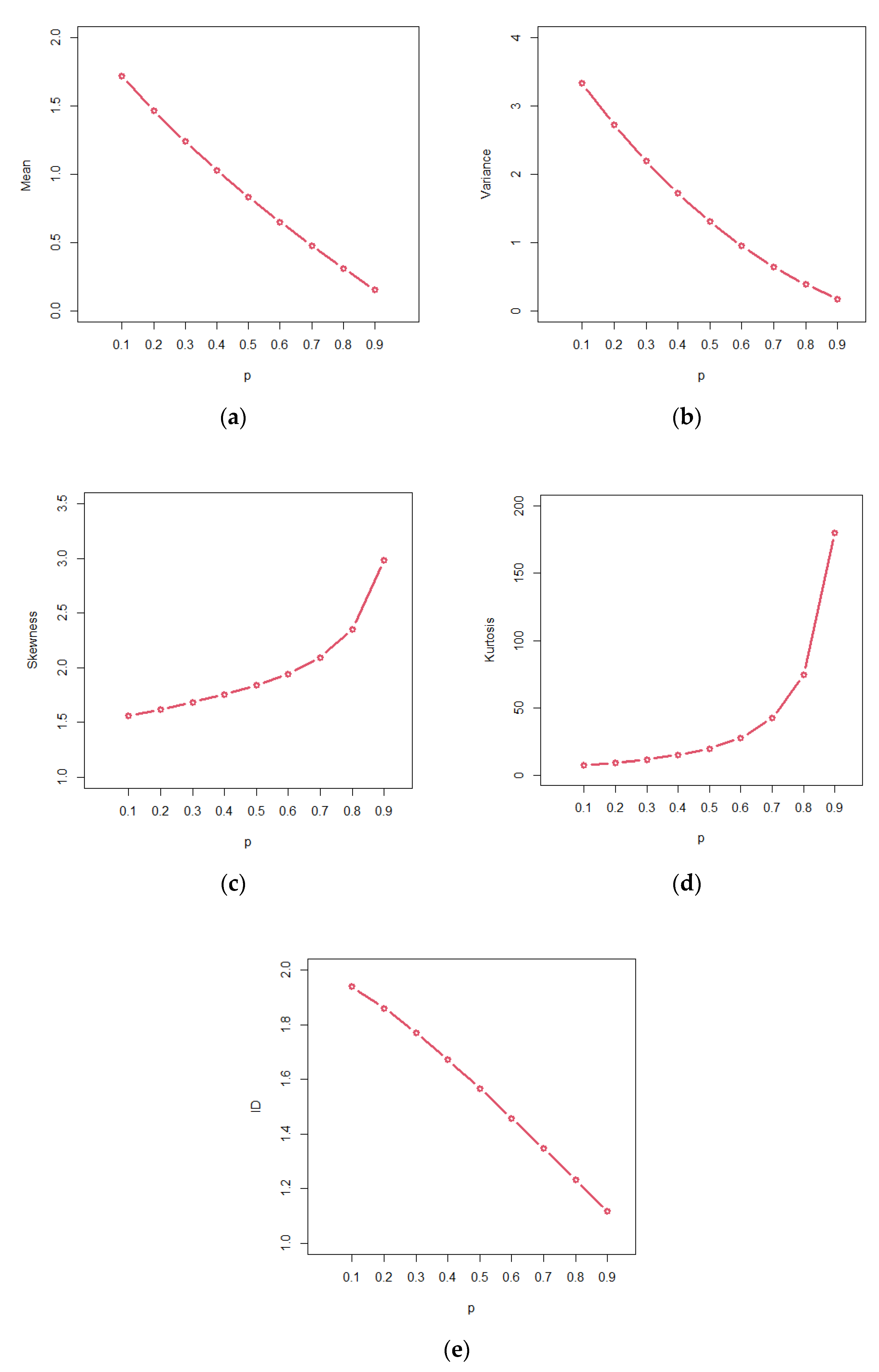
| Mean | 1.71818 | 1.4666 | 1.2384 | 1.0285 | 0.8333 | 0.6500 | 0.4764 | 0.3111 | 0.1526 |
| Variance | 3.3314 | 2.7288 | 2.1923 | 1.7191 | 1.3055 | 0.9475 | 0.6412 | 0.3832 | 0.1703 |
| Skewness | 1.5578 | 1.6186 | 1.6831 | 1.7542 | 1.8372 | 1.9427 | 2.0935 | 2.3522 | 2.9813 |
| Kurtosis | 7.7069 | 9.4991 | 11.8378 | 15.0902 | 19.9488 | 27.8656 | 42.3746 | 74.4447 | 180.1786 |
| ID | 1.9389 | 1.8606 | 1.770268 | 1.6714 | 1.5666 | 1.4576 | 1.3459 | 1.2317 | 1.1159 |
| p | p | ||
|---|---|---|---|
| 0.0001 | 1.87934 | 0.5 | 1.25943 |
| 0.01 | 1.86852 | 0.55 | 1.18391 |
| 0.03 | 1.84654 | 0.6 | 1.10402 |
| 0.05 | 1.82437 | 0.65 | 1.01888 |
| 0.07 | 1.80201 | 0.7 | 0.927315 |
| 0.09 | 1.77948 | 0.75 | 0.827736 |
| 0.11 | 1.75675 | 0.8 | 0.717861 |
| 0.14 | 1.72231 | 0.85 | 0.594157 |
| 0.17 | 1.6874 | 0.9 | 0.450497 |
| 0.2 | 1.652 | 0.95 | 0.273684 |
| 0.25 | 1.59181 | 0.96 | 0.231718 |
| 0.3 | 1.52994 | 0.97 | 0.186252 |
| 0.35 | 1.46611 | 0.98 | 0.135994 |
| 0.4 | 1.40002 | 0.99 | 0.078212 |
| 0.45 | 1.33128 | 0.999 | 0.0112562 |
| Distribution | MLE (SE) | MEASURES | |||
|---|---|---|---|---|---|
| AIC | CAIC | BIC | HQIC | ||
| BNDL (p) | 0.6283 (0.0129) | 2681.839 | 2681.844 | 2686.451 | 2683.616 |
| BDLD (p) | 0.6922 (0.0055) | 3092.3700 | 3092.3760 | 3096.9820 | 3094.1480 |
| Negative Binomial (n, k) | 17.2957, 2.9262 (4.7378, 0.0678) | 2824.156 | 2849.44 | 2833.38 | 2818.69 |
Publisher’s Note: MDPI stays neutral with regard to jurisdictional claims in published maps and institutional affiliations. |
© 2022 by the authors. Licensee MDPI, Basel, Switzerland. This article is an open access article distributed under the terms and conditions of the Creative Commons Attribution (CC BY) license (https://creativecommons.org/licenses/by/4.0/).
Share and Cite
Shafiq, S.; Khan, S.; Marzouk, W.; Gillariose, J.; Jamal, F. The Binomial–Natural Discrete Lindley Distribution: Properties and Application to Count Data. Math. Comput. Appl. 2022, 27, 62. https://doi.org/10.3390/mca27040062
Shafiq S, Khan S, Marzouk W, Gillariose J, Jamal F. The Binomial–Natural Discrete Lindley Distribution: Properties and Application to Count Data. Mathematical and Computational Applications. 2022; 27(4):62. https://doi.org/10.3390/mca27040062
Chicago/Turabian StyleShafiq, Shakaiba, Sadaf Khan, Waleed Marzouk, Jiju Gillariose, and Farrukh Jamal. 2022. "The Binomial–Natural Discrete Lindley Distribution: Properties and Application to Count Data" Mathematical and Computational Applications 27, no. 4: 62. https://doi.org/10.3390/mca27040062
APA StyleShafiq, S., Khan, S., Marzouk, W., Gillariose, J., & Jamal, F. (2022). The Binomial–Natural Discrete Lindley Distribution: Properties and Application to Count Data. Mathematical and Computational Applications, 27(4), 62. https://doi.org/10.3390/mca27040062