
On the Use of High-Order Shape Functions in the SAFE Method and Their Performance in Wave Propagation Problems

 , , , ,
Abstract
:1. Introduction
2. SAFE Method
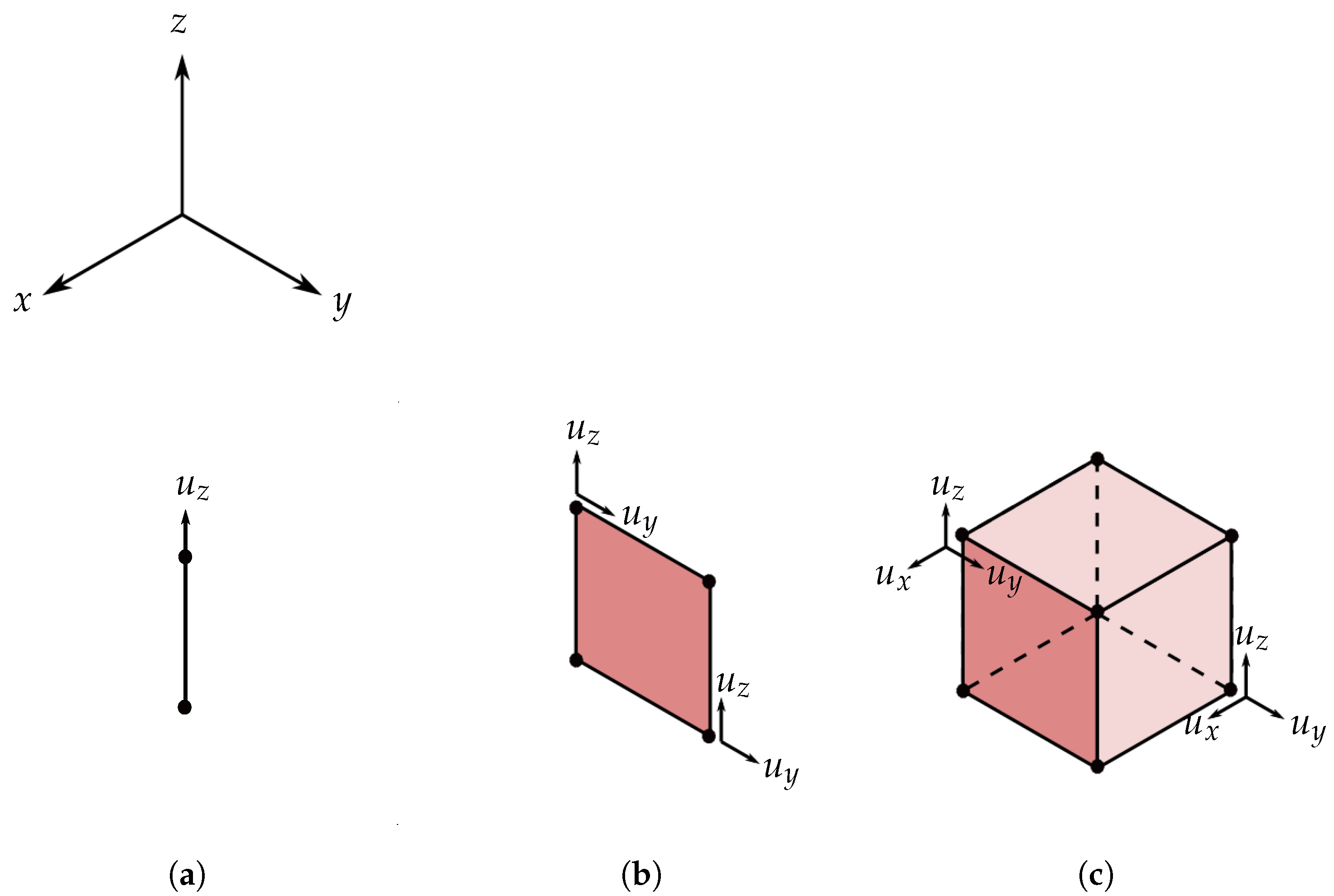
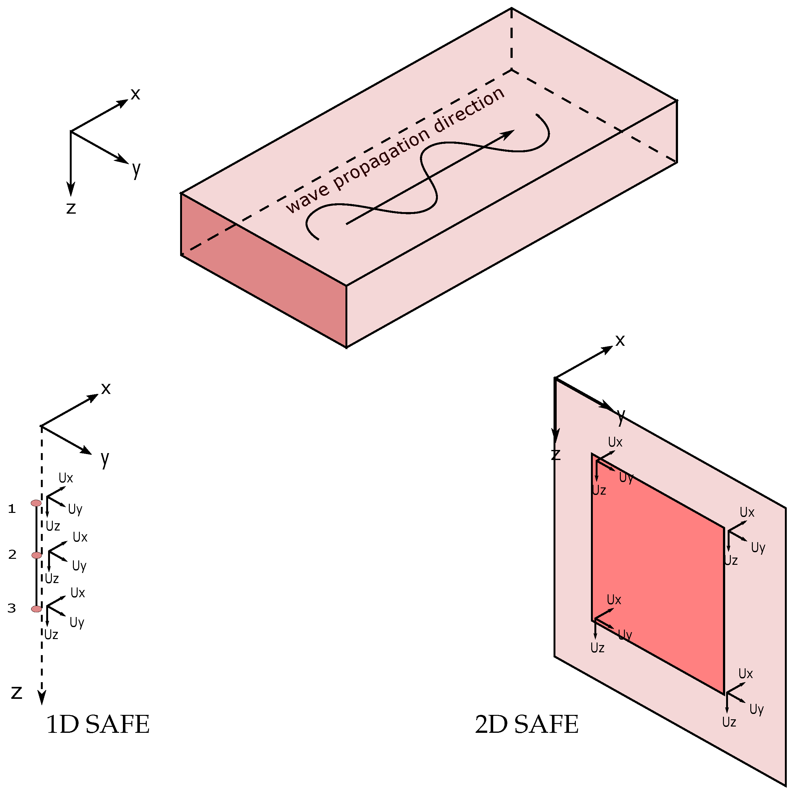
- 1D SAFE method:withand
- 2D SAFE method:withand
3. High-Order Shape Functions
- Standard shape functions based on Lagrange polynomials with equidistant nodal distribution:
- The Lagrange interpolation polynomials are defined as [63,64]is a p-th degree polynomial given by the product of p linear factors [65]. Moreover, represents the given set of points over a specified range, while is a particular point in that set. An equidistant distribution of the points over the interval , which is a typical for a local coordinate system of an element, is calculated by [66]:
- Spectral shape functions based on Lagrange polynomials with Gauss–Lobatto–Legendre (GLL) and Gauss–Lobatto–Chebyshev (GLC) nodal distributions:
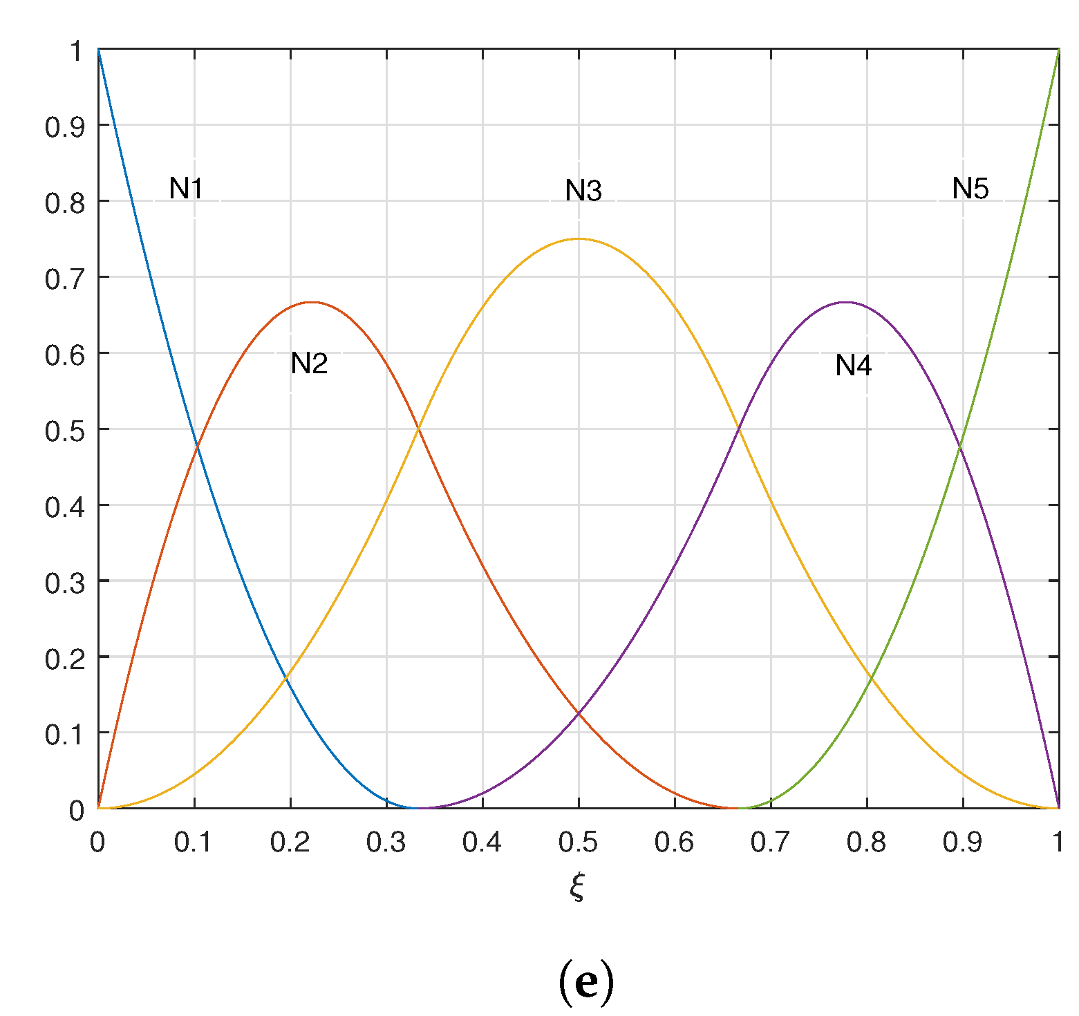
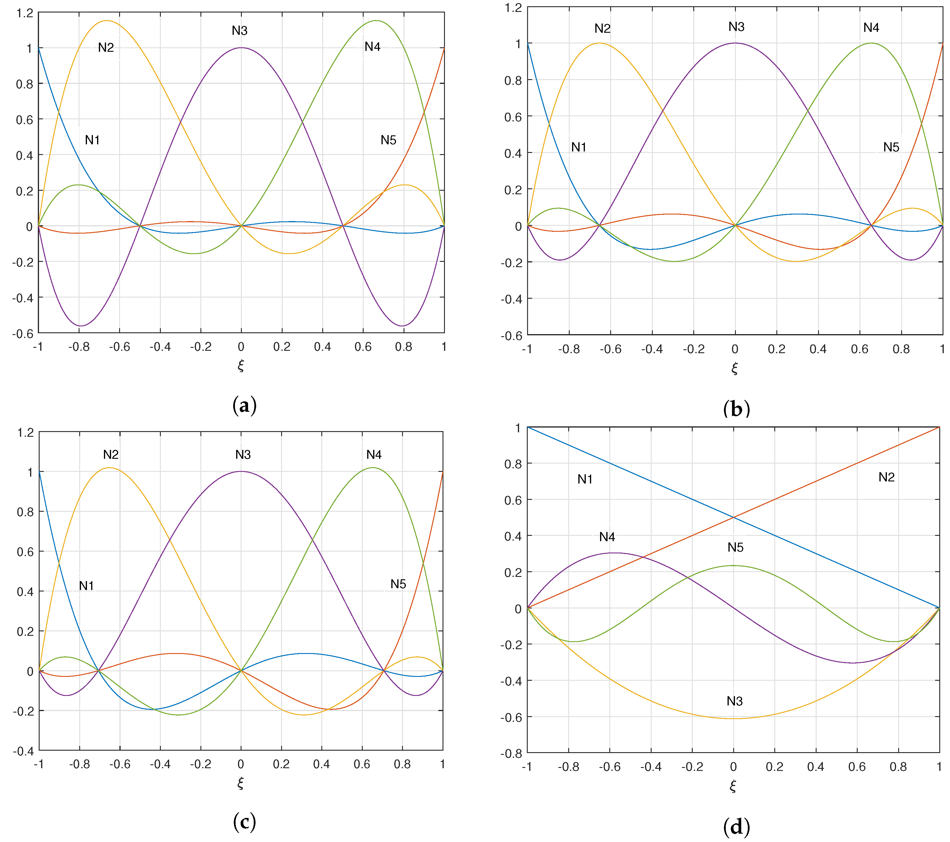
- Standard shape functions based on Lagrange polynomials defined using an equidistant nodal distribution lead to large oscillations and consequently to ill-conditioning [63,67]. This poor behavior of polynomial interpolation in equally spaced points is known as Runge’s phenomenon, which infers that increasing the order of shape functions does not necessarily incur lower errors [63,68]. Therefore, in order to circumvent this problem, non-equidistant nodal distributions such as GLL points [69] and GLC [70] have been proposed. In Figure 2a–c, the shape functions of a fifth order Lagrange polynomial based on equidistant, GLL, and GLC nodal distributions are depicted, respectively. The GLL and GLC nodal distributions along with high-order Lagrange polynomials are used in the SEM [63], which was first presented by Patera et al. in the field of fluid dynamics [71]. Note that SEM with GLL points has a special characteristic besides low numerical dispersion. The mass matrix for this particular spectral element is approximated through reduced integration by a diagonal matrix [67,72]. However, the SEM suffers from the fact that, for increasing the order of the shape functions, an additional node should be inserted and consequently all other internal nodes are repositioned and the coefficient matrices must be re-computed [73,74]. To derive the GLL points, we choose the roots of the first derivative of a p-th degree Legendre polynomial plus the endpoints located at and [63]where denotes the aforementioned roots.
- Hierarchic shape functions based on the normalized integrals of the Legendre-polynomials:
- Hierarchic shape functions are mainly used in the p-version of FEM. The principal difference between hierarchical shape functions and other sets of shape functions lies in the fact that in the hierarchic case the new DOFs are added to the existing ones without changing the existing DOFs. Thus, all lower order shape functions are contained in the higher order basis as depicted in Figure 2d. Unlike the previously discussed shape functions, where all the shape functions are of the same order, the order of the hierarchic shape functions increases incrementally starting from the first two linear shape functions. The one-dimensional, hierarchic shape functions consist of two nodal shape functions and various internal shape functionswhich are normalized integrals of Legendre polynomials. Here, is a Legendre polynomial of order . Note that, in p-FEM, not all DOFs represent actual nodal displacements [72], instead they are actually only unknowns of the high-order ansatz space [73].
- Non-Uniform Rational Basis Splines:
- In standard isoparamteric approaches, the shape functions used on an elemental level to discretize the geometry under investigation are only approximate in nature. Hence, numerical errors in geometries description are cause, which is especially important for geometries including curved surfaces. Thus, Hughes et al. [75] introduced the socalled isogeometric analysis in which nonuniform rational B-splines (NURBS) are used as shape functions. NURBS are frequently used for describing the geometry in a computer aided design (CAD) and computer aided manufacturing (CAM) applications [75,76]. NURBS are a generalization of B-splines and are derived by projecting B-splines from into , where d represents the dimensionality of the problem. A NURBS entity can be defined using knot vectors and a series of control points. The term ‘knot vector’ can be deceiving as a knot vector is simply a list of non-decreasing entries called knots and is not a real vector. A knot vector (see the example below),defines the parametric space of a univariate NURBS entity (curve). In Equation (38), p and n represent the degree of the NURBS and the number of control points, respectively. A knot vector can range between any two real numbers, but it is very common to choose 0 and 1 as the lower- and upper-bounds of the parametric space. The space between two adjacent knots is called a knot span. Non-zero knot spans can be compared to elements in the classical finite element method. Knot vectors control the discretization of the geometry and also the continuity across the elements, whereas the control points are responsible for all the changes regarding the geometry. As a rule, a degree p NURBS has -continuity across the knot spans inside a patch, where m is the knot multiplicity in the knot vector. (Remark: NURBS patches are geometrically simple domains within which the element types and material models are presumed to be uniform.) The first and the last knots in the knot vectors of ‘open NURBS’ which are considered in this study have a multiplicity of , making their ends -continuous. For instance, the knot vector in Equation (38) represents a quadratic () univariate NURBS with two elements, where the continuity on knots , and is . A univariate NURBS is a rational generalization of a B-spline curve. For a degree p NURBS curve, the corresponding shape function is given by (see [77,78])where is the weighting function, represents the weights associated with the control points, and, finally, denotes the standard B-spline basis functions in the parametric space. Shape functions of basis splines are defined by the Cox–de Boor recursion formula:For ,For ,Refinement of NURBS entities is usually achieved by modifying the underlying B-spline (in ). There are three methods to refine a B-spline/NURBS entity:
- -
- Knot insertion: Additional knots are added to the knot vector, increasing the number of control points and basis functions. Knot insertion is closely related to h-refinement in the classical FEM, as inserting additional knots increases the number of finite elements in the resulting discretization. Each knot must be inserted p times, maintaining the -continuity between the elements, to resemble the classical h-refinement technique completely,
- -
- Degree elevation: The polynomial degree of the NURBS entity is increased, while preserving the continuity of the curve. In the case where the continuity between the elements is , degree elevation is equivalent to the p-refinement technique in the classical FEM.
- -
- k-refinement: Combination of knot insertion and degree elevation techniques. To better understand the k-refinement technique, one ought to note that knot insertion and degree elevation are not commutative. In other words, the order in which the refinement techniques are applied plays a crucial role in achieving the desired properties of the final discretization. k-refinement makes it possible to increase the polynomial degree of the NURBS object, while increasing its continuity as well. This leads to more accurate results using less control points. To achieve the highest level of its benefits, i.e., continuity of the basis between the elements of the refined discretization, one needs to start with one element in the coarsest discretization, elevate the basis to the desired degree and then insert the additional knots to introduce the elements. On the other hand, inserting knots first on a lower degree and then elevating the degree will lead to lower continuity across the elements (, if one starts from a linear discretization) and more control points. This technique does not have any equivalents in the classical FEM.
4. Results and Discussion
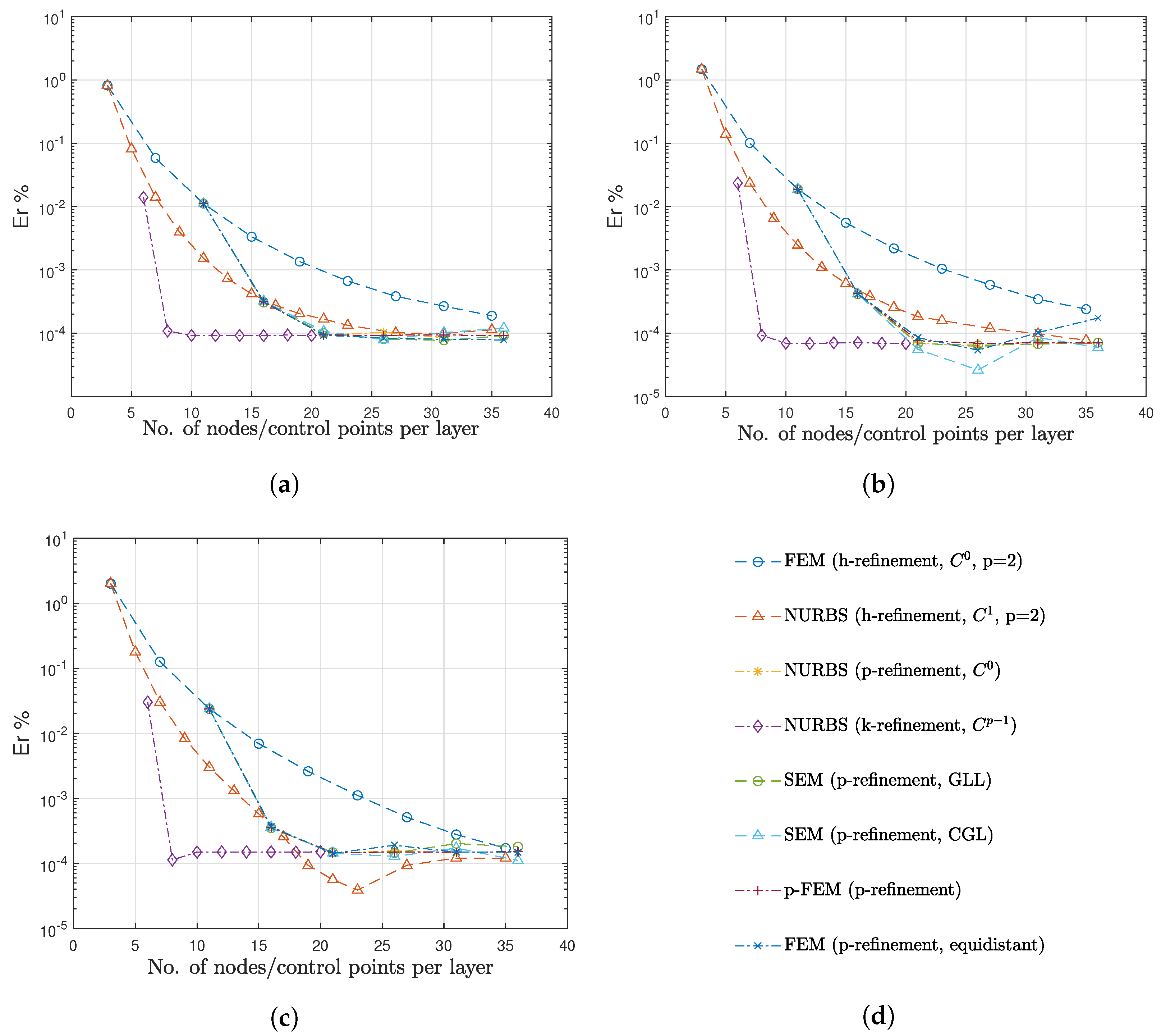
- h-refinement approach using:
- second order standard shape functions based on Lagrange polynomials with equidistant nodal distribution (FEM);
- second order NURBS shape functions with -continuity (NURBS-based IGA);
- p-refinement approach using high-order shape functions ():
- standard shape functions based on Lagrange polynomials with equidistant nodal distribution;
- spectral shape functions based on Lagrange polynomials with Gauss-Lobatto-Legendre nodal distribution (SEM);
- spectral shape functions based on Lagrange polynomials with Gauss-Lobatto-Chebyshev nodal distribution (SEM);
- hierarchic shape functions based on the normalized integrals of the Legendre-polynomials (p-FEM);
- NURBS with -continuity (NURBS-based IGA)
- k-refinement approach using:
- NURBS with -continuity (NURBS-based IGA).
4.1. Isotropic Case Study
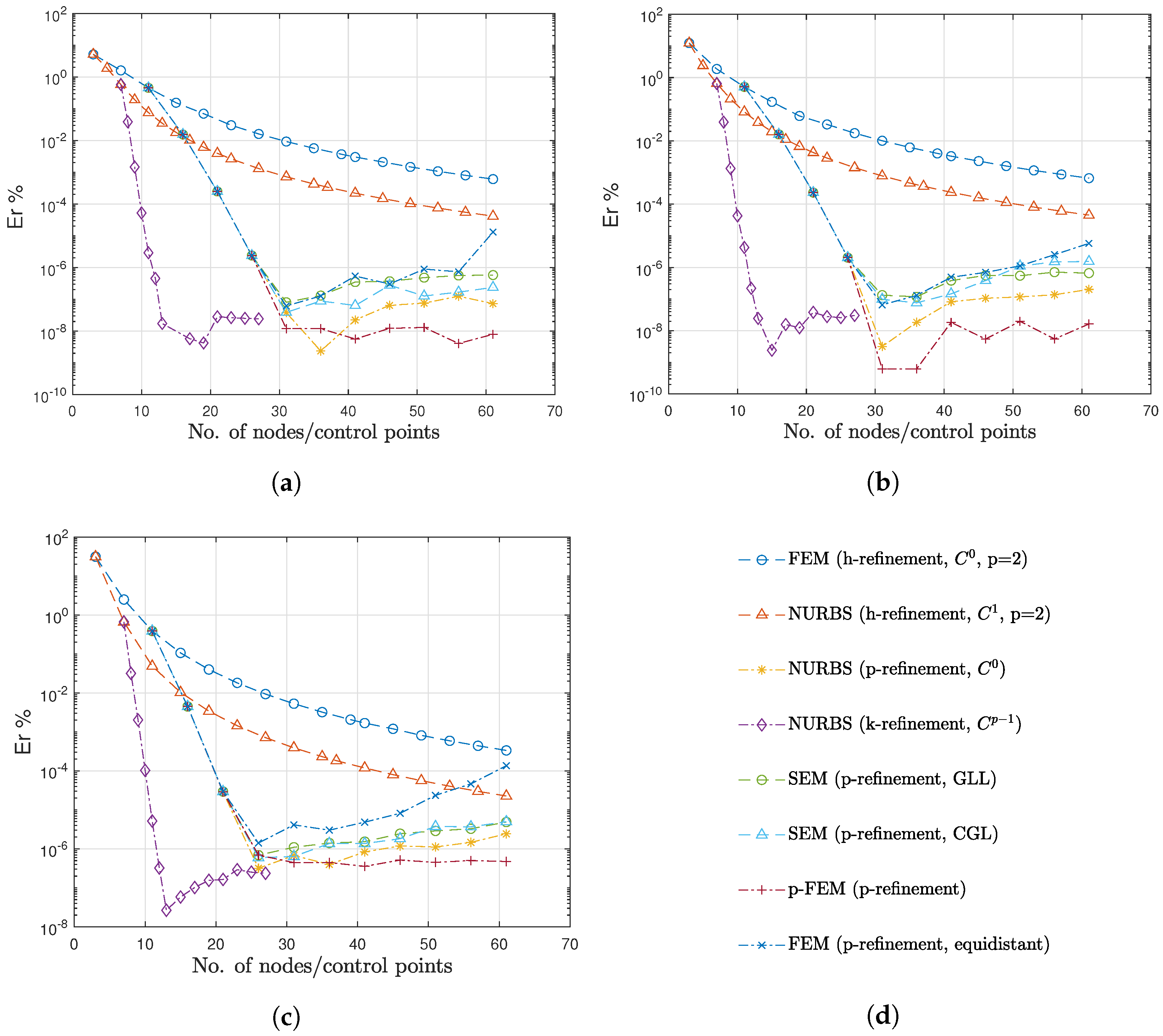
- The highest convergence rate is achieved by the approach which takes advantage of NURBS shape functions of degree p with continuity between elements and the k-refinement technique. Here, a total of five elements (non-zero knot spans) were considered, and, in each step, the degree of the shape functions and their continuity is increased.
- Among the high-order shape functions with continuity between the elements, the hierarchical shape functions (p-FEM method; purple dash-dotted curve with ‘+’ markers) show the best performance. The attainable error level is slightly lower compared to the other methods. Here, no divergence is observed when the order of the shape functions is repeatedly increased. In the following order, the other continuous approaches can be ranked: NURBS shape functions (yellow dash-dotted curve with asterix markers), spectral shape functions (with GLL or GLC points; green dashed curve with ‘o’ markers or cyan dashed curve with triangle markers), and standard shape functions (dark blue dash-dotted curve with ‘x’ markers), respectively. As mentioned previously, it may also be observed that, as the shape function order increases in the standard shape functions with equidistant nodal distribution, the error increases, which is related to Runge’s phenomenon. Additionally, it should be noted that, in the thickness of the plate, a constant number of five elements were considered during the p-refinement approach.
- Finally, the h-refinement technique shows the poorest performance among the other presented approaches. The methods which include h-refinement technique second order shape functions with continuity (FEM, blue dashed line with ‘o’ marker) and continuity (IGA, red dashed line with rectangular marker) were considered and the number of elements increased in each step. As it can be observed, the approach which takes advantage of continuity shows better performance than the standard FEM with continuity between the elements, which is the expected behavior.
4.2. Composite Case Study
5. Conclusions
Author Contributions
Funding
Data Availability Statement
Conflicts of Interest
Abbreviations
| SAFE | Semi-Analytical Finite Element Method |
| DOF | Degree of Freedom |
| FEM | Finite Element Method |
| SEM | Spectral Element Method |
| IGA | Isogeometric Analysis |
| 1D SAFE | One Dimensional Semi-Analytical Finite Element Method |
| 2D SAFE | Two Dimensional Semi-Analytical Finite Element Method |
| SHM | Structural Health Monitoring |
| FEA | Finite Element Analysis |
| GLL | Gauss–Lobatto–Legendre |
| GLC | Gauss–Lobatto–Chebyshev |
| p-FEM | p-Version of Finite Element Method |
| NURBS | Nonuniform Rational B-Splines |
| CAD | Computer Aided Design |
| CAM | Computer Aided Manufacturing |
Appendix A. Basic methods and definitions
Appendix A.1. Eigenvalue Problem Solution and Analysis
- Assign real values to the circular frequency and solve either the second-order, cf. Equation (25), or the first-order eigenvalue problem, cf. Equation (26). The eigenvalues calculated in this case fall in one of the following three categories:
- (a)
- Real eigenvalues () corresponding to propagating waves;
- (b)
- Complex eigenvalues () corresponding to evanescent waves; (Remark: Evanescent waves are a type of waves whose energy is spatially concentrated in the vicinity of the source, i.e., after travelling a certain distance in the waveguide their amplitude becomes negligible [1].)
- (c)
- Imaginary eigenvalues () corresponding to standing waves. (Remark: Standing waves or non-oscillating evanescent waves are stationary in the structure and do not transport energy.)
- Assign values to the wavenumber and solve the second-order eigenvalue problem given by Equation (25). It should be mentioned that, if real values are assigned to the wavenumber, only propagating modes are being considered, and, likewise, if we assign imaginary values to the wavenumber, only standing waves may be studied.
Appendix A.2. Phase Velocity and Group Velocity
Appendix A.3. Cut-Off Frequency
Appendix B. Mode Identification Approaches
- 1
- Quadratic polynomial [9]:Considering the fact that in general one may fit any points by a polynomial of p-th degree, Lagrange polynomials constitute a viable choice [63]. The fitted polynomial takes the formwhere the cardinal functions are expressed asAccording to this definition, if we consider a second-order Lagrange polynomial for the wavenumber k at the desired frequency , it is extrapolated by using three points as follows:By considering a constant frequency step, Equation (A8) may be further simplified:
- 2
- Taylor series expansion:Besides Lagrange polynomials, we can also make use of a Taylor series expansion to derive the extrapolating polynomial. If we consider , the p-th order Taylor expansion of f is defined as [86]where is the remainder, and the factor is defined asIf we consider the terms up to the third-order, the wavenumber may be extrapolated using the following expression:where . By using the backward difference method, the derivatives of the function are derived as follows:
- 3
- Padé series expansion:Another extrapolation method, which has been proposed by Gravenkamp et al. [80] for tracing dispersion curves, uses Padé expansions. A Padé approximation of f is a rational function with a numerator of degree L and denominator of degree M, determined such that its power expansion matches up to including the power . Considering , the Padé expansion of f may be presented as follows:where is the remainder of order , and is called the Padé approximation of order of function f. The coefficients of the Padé expansion may be derived by replacing the left term in Equation (A16) by a Taylor series using Equation (A10) [86]:where . By multiplying both sides by the denominator of the term on the right-hand-side of the equation and comparing the coefficients of the terms with the same power, a set of linear algebraic equations is derived, which may be solved in order to calculate the Padé expansion coefficients. Using this method, the following set of equations may be derived for a Padé expansion of order [1/2] using Equation (A17):For a Padé expansion of order [1/2], we obtain . By solving the set of algebraic equations, the coefficients of a Padé expansion of order [1/2] arewhere are given by Equations (A11) and (A13)–(A15). Consequently, by replacing these coefficients in Equation (A16), the Padé expansion of order [1/2] of the wavenumber may be expressed as:
References
- Bartoli, I.; Marzani, A.; di Scalea, F.L.; Viola, E. Modeling wave propagation in damped waveguides of arbitrary cross-section. J. Sound Vib. 2006, 295, 685–707. [Google Scholar] [CrossRef]
- Marzani, A.; Viola, E.; Bartoli, I.; di Scalea, F.L.; Rizzo, P. A semi-analytical finite element formulation for modeling stress wave propagation in axisymmetric damped waveguides. J. Sound Vib. 2008, 318, 488–505. [Google Scholar] [CrossRef]
- Marzani, A. Time–transient response for ultrasonic guided waves propagating in damped cylinders. Int. J. Solids Struct. 2008, 45, 6347–6368. [Google Scholar] [CrossRef]
- Schmiechen, P. Travelling Wave Speed Coincidence. Ph.D. Thesis, University of London, London, UK, 1997. [Google Scholar]
- Marburg, S.; Nolte, B. Computational Acoustics of Noise Propagation in Fluids—Finite and Boundary Element Methods; Springer: Berlin/Heidelberg, Germany, 2008. [Google Scholar] [CrossRef]
- Bathe, K.J. Finite Element Procedures; Prentice Hall: Hoboken, NJ, USA, 2006. [Google Scholar]
- Bartoli, I.; Lanza di Scalea, F.; Fateh, M.; Viola, E. Modeling guided wave propagation with application to the long-range defect detection in railroad tracks. Ndt E Int. 2005, 38, 325–334. [Google Scholar] [CrossRef]
- Willberg, C.; Duczek, S.; Perez, J.V.; Schmicker, D.; Gabbert, U. Comparison of different higher order finite element schemes for the simulation of Lamb waves. Comput. Methods Appl. Mech. Eng. 2012, 241–244, 246–261. [Google Scholar] [CrossRef]
- Lowe, M. Matrix techniques for modeling ultrasonic waves in multilayered media. IEEE Trans. Ultrason. Ferroelectr. Freq. Control. 1995, 42, 525–542. [Google Scholar] [CrossRef]
- Rokhlin, S.I.; Wang, L. Stable recursive algorithm for elastic wave propagation in layered anisotropic media: Stiffness matrix method. J. Acoust. Soc. Am. 2002, 112, 822–834. [Google Scholar] [CrossRef]
- Astaneh, A.V.; Guddati, M.N. Dispersion analysis of composite acousto-elastic waveguides. Compos. Part Eng. 2017, 130, 200–216. [Google Scholar] [CrossRef]
- Joseph, R.; Li, L.; Haider, M.F.; Giurgiutiu, V. Hybrid SAFE-GMM approach for predictive modeling of guided wave propagation in layered media. Eng. Struct. 2019, 193, 194–206. [Google Scholar] [CrossRef]
- Su, Z.; Ye, L.; Lu, Y. Guided Lamb waves for identification of damage in composite structures: A review. J. Sound Vib. 2006, 295, 753–780. [Google Scholar] [CrossRef]
- Willberg, C.; Duczek, S.; Vivar-Perez, J.M.; Ahmad, Z.A.B. Simulation Methods for Guided Wave-Based Structural Health Monitoring: A Review. Appl. Mech. Rev. 2015, 67. [Google Scholar] [CrossRef]
- Aalami, B. Waves in Prismatic Guides of Arbitrary Cross Section. J. Appl. Mech. 1973, 40, 1067–1072. [Google Scholar] [CrossRef]
- Lagasse, P.E. Higher-order finite-element analysis of topographic guides supporting elastic surface waves. J. Acoust. Soc. Am. 1973, 53, 1116–1122. [Google Scholar] [CrossRef]
- Zienkiewicz, O.C. The Finite Element Method in Engineering Science; McGraw-Hill: London, UK; New York, NY, USA, 1971. [Google Scholar]
- Mazzotti, M.; Bartoli, I.; Miniaci, M.; Marzani, A. Wave dispersion in thin-walled orthotropic waveguides using the first order shear deformation theory. Thin-Walled Struct. 2016, 103, 128–140. [Google Scholar] [CrossRef]
- Hladky-Hennion, A.C. Finite element analysis of the propagation of acoustic waves in waveguides. J. Sound Vib. 1996, 194, 119–136. [Google Scholar] [CrossRef]
- Damljanović, V.; Weaver, R.L. Forced response of a cylindrical waveguide with simulation of the wavenumber extraction problem. J. Acoust. Soc. Am. 2004, 115, 1582–1591. [Google Scholar] [CrossRef]
- Loveday, P.W. Simulation of piezoelectric excitation of guided waves using waveguide finite elements. IEEE Trans. Ultrason. Ferroelectr. Freq. Control. 2008, 55, 2038–2045. [Google Scholar] [CrossRef]
- Coccia, S.; Bartoli, I.; Marzani, A.; di Scalea, F.L.; Salamone, S.; Fateh, M. Numerical and experimental study of guided waves for detection of defects in the rail head. Ndt Int. 2011, 44, 93–100. [Google Scholar] [CrossRef]
- Treyssède, F. Elastic waves in helical waveguides. Wave Motion 2008, 45, 457–470. [Google Scholar] [CrossRef]
- Cong, M.; Wu, X.; Liu, R. Dispersion analysis of guided waves in the finned tube using the semi-analytical finite element method. J. Sound Vib. 2017, 401, 114–126. [Google Scholar] [CrossRef]
- Mazzotti, M.; Bartoli, I.; Marzani, A.; Viola, E. A coupled SAFE-2.5D BEM approach for the dispersion analysis of damped leaky guided waves in embedded waveguides of arbitrary cross-section. Ultrasonics 2013, 53, 1227–1241. [Google Scholar] [CrossRef] [PubMed]
- Mazzotti, M.; Marzani, A.; Bartoli, I. Dispersion analysis of leaky guided waves in fluid-loaded waveguides of generic shape. Ultrasonics 2014, 54, 408–418. [Google Scholar] [CrossRef] [PubMed]
- Treyssède, F.; Nguyen, K.; Bonnet-BenDhia, A.S.; Hazard, C. Finite element computation of trapped and leaky elastic waves in open stratified waveguides. Wave Motion 2014, 51, 1093–1107. [Google Scholar] [CrossRef]
- Nguyen, K.; Treyssède, F.; Hazard, C. Numerical modeling of three-dimensional open elastic waveguides combining semi-analytical finite element and perfectly matched layer methods. J. Sound Vib. 2015, 344, 158–178. [Google Scholar] [CrossRef]
- Zuo, P.; Yu, X.; Fan, Z. Numerical modeling of embedded solid waveguides using SAFE-PML approach using a commercially available finite element package. Ndt Int. 2017, 90, 11–23. [Google Scholar] [CrossRef]
- Duan, W.; Kirby, R.; Mudge, P.; Gan, T.H. A one-dimensional, numerical approach for computing the eigenmodes of elastic waves in buried pipelines. J. Sound Vib. 2016, 384, 177–193. [Google Scholar] [CrossRef]
- Matuszyk, P.J. Modeling of guided circumferential SH and Lamb-type waves in open waveguides with semi-analytical finite element and Perfectly Matched Layer method. J. Sound Vib. 2017, 386, 295–310. [Google Scholar] [CrossRef]
- Zuo, P.; Fan, Z. SAFE-PML approach for modal study of waveguides with arbitrary cross sections immersed in inviscid fluid. J. Sound Vib. 2017, 406, 181–196. [Google Scholar] [CrossRef]
- tian Deng, Q.; chun Yang, Z. Propagation of guided waves in bonded composite structures with tapered adhesive layer. Appl. Math. Model. 2011, 35, 5369–5381. [Google Scholar] [CrossRef]
- Mei, H.; Giurgiutiu, V. Predictive 1D and 2D guided-wave propagation in composite plates using the SAFE approach. In Proceedings of the Health Monitoring of Structural and Biological Systems XII, Denver, CO, USA, 5–8 March 2018; Kundu, T., Ed.; International Society for Optics and Photonics: Bellingham, WA, USA, 2018; Volume 10600, pp. 215–225. [Google Scholar] [CrossRef]
- Duan, W.; Gan, T.H. Investigation of guided wave properties of anisotropic composite laminates using a semi-analytical finite element method. Compos. Part Eng. 2019, 173, 106898. [Google Scholar] [CrossRef]
- Cui, R.; di Scalea, F.L. On the identification of the elastic properties of composites by ultrasonic guided waves and optimization algorithm. Compos. Struct. 2019, 223, 110969. [Google Scholar] [CrossRef]
- Inoue, D.; Hayashi, T. Transient analysis of leaky Lamb waves with a semi-analytical finite element method. Ultrasonics 2015, 62, 80–88. [Google Scholar] [CrossRef] [PubMed]
- Duan, W.; Kirby, R. Guided wave propagation in buried and immersed fluid-filled pipes: Application of the semi analytic finite element method. Comput. Struct. 2019, 212, 236–247. [Google Scholar] [CrossRef]
- Han, X.; Liu, G.R.; Xi, Z.C.; Lam, K.Y. Characteristics of waves in a functionally graded cylinder. Int. J. Numer. Methods Eng. 2002, 53, 653–676. [Google Scholar] [CrossRef]
- Hayashi, T.; Inoue, D. Calculation of leaky Lamb waves with a semi-analytical finite element method. Ultrasonics 2014, 54, 1460–1469. [Google Scholar] [CrossRef]
- Gavrić, L. Computation of propagative waves in free rail using a finite element technique. J. Sound Vib. 1995, 185, 531–543. [Google Scholar] [CrossRef]
- Hayashi, T.; Song, W.J.; Rose, J.L. Guided wave dispersion curves for a bar with an arbitrary cross-section, a rod and rail example. Ultrasonics 2003, 41, 175–183. [Google Scholar] [CrossRef]
- Damljanović, V.; Weaver, R.L. Propagating and evanescent elastic waves in cylindrical waveguides of arbitrary cross section. J. Acoust. Soc. Am. 2004, 115, 1572–1581. [Google Scholar] [CrossRef]
- Hayashi, T.; Tamayama, C.; Murase, M. Wave structure analysis of guided waves in a bar with an arbitrary cross-section. Ultrasonics 2006, 44, 17–24. [Google Scholar] [CrossRef]
- Predoi, M.V.; Castaings, M.; Hosten, B.; Bacon, C. Wave propagation along transversely periodic structures. J. Acoust. Soc. Am. 2007, 121, 1935–1944. [Google Scholar] [CrossRef]
- Loveday, P.W. Analysis of Piezoelectric Ultrasonic Transducers Attached to Waveguides Using Waveguide Finite Elements. IEEE Trans. Ultrason. Ferroelectr. Freq. Control. 2007, 54, 2045–2051. [Google Scholar] [CrossRef] [PubMed]
- Loveday, P.W. Semi-analytical finite element analysis of elastic waveguides subjected to axial loads. Ultrasonics 2009, 49, 298–300. [Google Scholar] [CrossRef] [PubMed]
- Mazzotti, M.; Marzani, A.; Bartoli, I.; Viola, E. Guided waves dispersion analysis for prestressed viscoelastic waveguides by means of the SAFE method. Int. J. Solids Struct. 2012, 49, 2359–2372. [Google Scholar] [CrossRef]
- Setshedi, I.I.; Loveday, P.W.; Long, C.S.; Wilke, D.N. Estimation of rail properties using semi-analytical finite element models and guided wave ultrasound measurements. Ultrasonics 2019, 96, 240–252. [Google Scholar] [CrossRef] [PubMed]
- Loveday, P.W.; Long, C.S.; Ramatlo, D.A. Mode repulsion of ultrasonic guided waves in rails. Ultrasonics 2018, 84, 341–349. [Google Scholar] [CrossRef]
- Onipede, O.; Dong, S.; Kosmatka, J. Natural vibrations and waves in pretwisted rods. Compos. Eng. 1994, 4, 487–502. [Google Scholar] [CrossRef]
- Mazúch, T. Wave dispersion modelling in anisotropic shells and rods by the finite element method. J. Sound Vib. 1996, 198, 429–438. [Google Scholar] [CrossRef]
- Volovoi, V.; Hodges, D.; Berdichevsky, V.; Sutyrin, V. Dynamic dispersion curves for non-homogeneous, anisotropic beams with cross-sections of arbitrary geometry. J. Sound Vib. 1998, 215, 1101–1120. [Google Scholar] [CrossRef]
- Treyssède, F.; Laguerre, L. Investigation of elastic modes propagating in multi-wire helical waveguides. J. Sound Vib. 2010, 329, 1702–1716. [Google Scholar] [CrossRef]
- Düster, A. High Order Finite Elements for Three-Dimensional, Thin-Walled Nonlinear Continua. Ph.D. Thesis, Technical University Munich, Munich, Germany, 2002. [Google Scholar]
- Rezaiee-Pajand, M.; Gharaei-Moghaddam, N.; Ramezani, M. Higher-order assumed strain plane element immune to mesh distortion. Eng. Comput. 2020. ahead-of-print. [Google Scholar] [CrossRef]
- Kalkowski, M.K.; Muggleton, J.M.; Rustighi, E. Axisymmetric semi-analytical finite elements for modelling waves in buried/submerged fluid-filled waveguides. Comput. Struct. 2018, 196, 327–340. [Google Scholar] [CrossRef]
- Xiao, D.; Han, Q.; Liu, Y.; Li, C. Guided wave propagation in an infinite functionally graded magneto-electro-elastic plate by the Chebyshev spectral element method. Compos. Struct. 2016, 153, 704–711. [Google Scholar] [CrossRef]
- Treyssède, F. Spectral element computation of high-frequency leaky modes in three-dimensional solid waveguides. J. Comput. Phys. 2016, 314, 341–354. [Google Scholar] [CrossRef]
- Seyfaddini, F.; Nguyen, V.H. NURBS-enriched semi-analytical finite element method (SAFE) for calculation of wave dispersion in heterogeneous waveguides. In Proceedings of the 24e Congrès Français de Mécanique, Brest, France, 26–30 August 2019. [Google Scholar]
- Seyfaddini, F.; Nguyen-Xuan, H.; Nguyen, V.H. A semi-analytical isogeometric analysis for wave dispersion in functionally graded plates immersed in fluids. Acta Mech. 2021, 232, 15–32. [Google Scholar] [CrossRef]
- Seyfaddini, F.; Nguyen-Xuan, H.; Nguyen, V.H. Semi-analytical IGA-based computation of wave dispersion in fluid-coupled anisotropic poroelastic plates. Int. J. Mech. Sci. 2021, 212, 106830. [Google Scholar] [CrossRef]
- Boyd, J.P. Chebyshev and Fourier Spectral Methods, 2nd ed.; Dover: Mineola, NY, USA, 2001. [Google Scholar]
- Atkinson, K.E. An Introduction to Numerical Analysis, 2nd ed.; John Wiley & Sons: Hoboken, NJ, USA, 1989; p. xvi+693. [Google Scholar]
- Rao, S. The Finite Element Method in Engineering, 5th ed.; Elsevier Inc.: Amsterdam, The Netherlands, 2010. [Google Scholar] [CrossRef]
- Zienkiewicz, O.; Taylor, R. Finite Element Method: Volume 1—The Basis, 5th ed.; Butterworth-Heinemann: Oxford, UK, 2000. [Google Scholar]
- Seriani, G.; Oliveira, S. Numerical Modeling of mechanical wave propagation. Riv. Del Nuovo C. 2020, 43, 459–514. [Google Scholar] [CrossRef]
- Trefethen, L.; Weideman, J. Two results on polynomial interpolation in equally spaced points. J. Approx. Theory 1991, 65, 247–260. [Google Scholar] [CrossRef]
- Zrahia, U.; Bar-Yoseph, P. Space-time spectral element method for solution of second-order hyperbolic equations. Comput. Methods Appl. Mech. Eng. 1994, 116, 135–146. [Google Scholar] [CrossRef]
- Seriani, G.; Priolo, E. Spectral element method for acoustic wave simulation in heterogeneous media. Finite Elem. Anal. Des. 1994, 16, 337–348. [Google Scholar] [CrossRef]
- Patera, A.T. A spectral element method for fluid dynamics: Laminar flow in a channel expansion. J. Comput. Phys. 1984, 54, 468–488. [Google Scholar] [CrossRef]
- Duczek, S.; Gravenkamp, H. Mass lumping techniques in the spectral element method: On the equivalence of the row-sum, nodal quadrature, and diagonal scaling methods. Comput. Methods Appl. Mech. Eng. 2019, 353, 516–569. [Google Scholar] [CrossRef]
- Vu, T.H.; Deeks, A.J. Use of higher-order shape functions in the scaled boundary finite element method. Int. J. Numer. Methods Eng. 2006, 65, 1714–1733. [Google Scholar] [CrossRef]
- Zienkiewicz, O.; Taylor, R.; Zhu, J. The Finite Element Method Set: Its Basis and Fundamentals, 6th ed.; Butterworth-Heinemann: Oxford, UK, 2005; pp. 103–137. [Google Scholar] [CrossRef]
- Hughes, T.; Cottrell, J.; Bazilevs, Y. Isogeometric analysis: CAD, finite elements, NURBS, exact geometry and mesh refinement. Comput. Methods Appl. Mech. Eng. 2005, 194, 4135–4195. [Google Scholar] [CrossRef]
- Agrawal, V.; Gautam, S.S. IGA: A Simplified Introduction and Implementation Details for Finite Element Users. J. Inst. Eng. Ser. 2019, 100, 561–585. [Google Scholar] [CrossRef]
- Cottrell, J.A.; Hughes, T.J.R.; Bazilevs, Y. NURBS as a Pre-Analysis Tool: Geometric Design and Mesh Generation. In Isogeometric Analysis; John Wiley & Sons, Ltd.: Hoboken, NJ, USA, 2009; pp. 19–68. [Google Scholar] [CrossRef]
- Piegl, L.; Tiller, W. The NURBS Book, 2nd ed.; Springer: New York, NY, USA, 1997. [Google Scholar]
- German Aerospace Center (DLR) Institute of Structures and Design, Center for Lightweight Production Technology Augsburg. The Dispersion Calculator: A Free Software for Calculating Dispersion Curves of Guided Waves in Multilayered Composites 2018. Available online: https://www.dlr.de/zlp/en/desktopdefault.aspx/tabid-14332/24874_read-61142/ (accessed on 1 June 2022).
- Gravenkamp, H.; Birk, C.; Song, C. The computation of dispersion relations for axisymmetric waveguides using the Scaled Boundary Finite Element Method. Ultrasonics 2014, 54, 1373–1385. [Google Scholar] [CrossRef]
- Mei, H.; Giurgiutiu, V. Guided wave excitation and propagation in damped composite plates. Struct. Health Monit. 2019, 18, 690–714. [Google Scholar] [CrossRef]
- Kudela, P.; Radzienski, M.; Fiborek, P.; Wandowski, T. Elastic constants identification of fibre-reinforced composites by using guided wave dispersion curves and genetic algorithm for improved simulations. Compos. Struct. 2021, 272, 114178. [Google Scholar] [CrossRef]
- Gravenkamp, H.; Saputra, A.A.; Duczek, S. High-order shape functions in the scaled boundary finite element method revisited. Arch. Comput. Methods Eng. 2019, 28, 473–494. [Google Scholar] [CrossRef]
- Finnveden, S. Evaluation of modal density and group velocity by a finite element method. J. Sound Vib. 2004, 273, 51–75. [Google Scholar] [CrossRef]
- Loveday, P.W.; Long, C.S. Time domain simulation of piezoelectric excitation of guided waves in rails using waveguide finite elements. Sensors and Smart Structures Technologies for Civil, Mechanical, and Aerospace Systems 2007; Tomizuka, M., Yun, C.B., Giurgiutiu, V., Eds.; International Society for Optics and Photonics: Bellingham, WA, USA, 2007; Volume 6529, pp. 316–325. [Google Scholar] [CrossRef]
- Simon Širca, M.H. Computational Methods in Physics, 2nd ed.; Springer: Berlin/Heidelberg, Germany, 2018. [Google Scholar] [CrossRef]


| Young’s Modulus () | Poisson’s Ratio | Density () |
|---|---|---|
| E | ||
| 73.1 | 0.33 | 2780 |
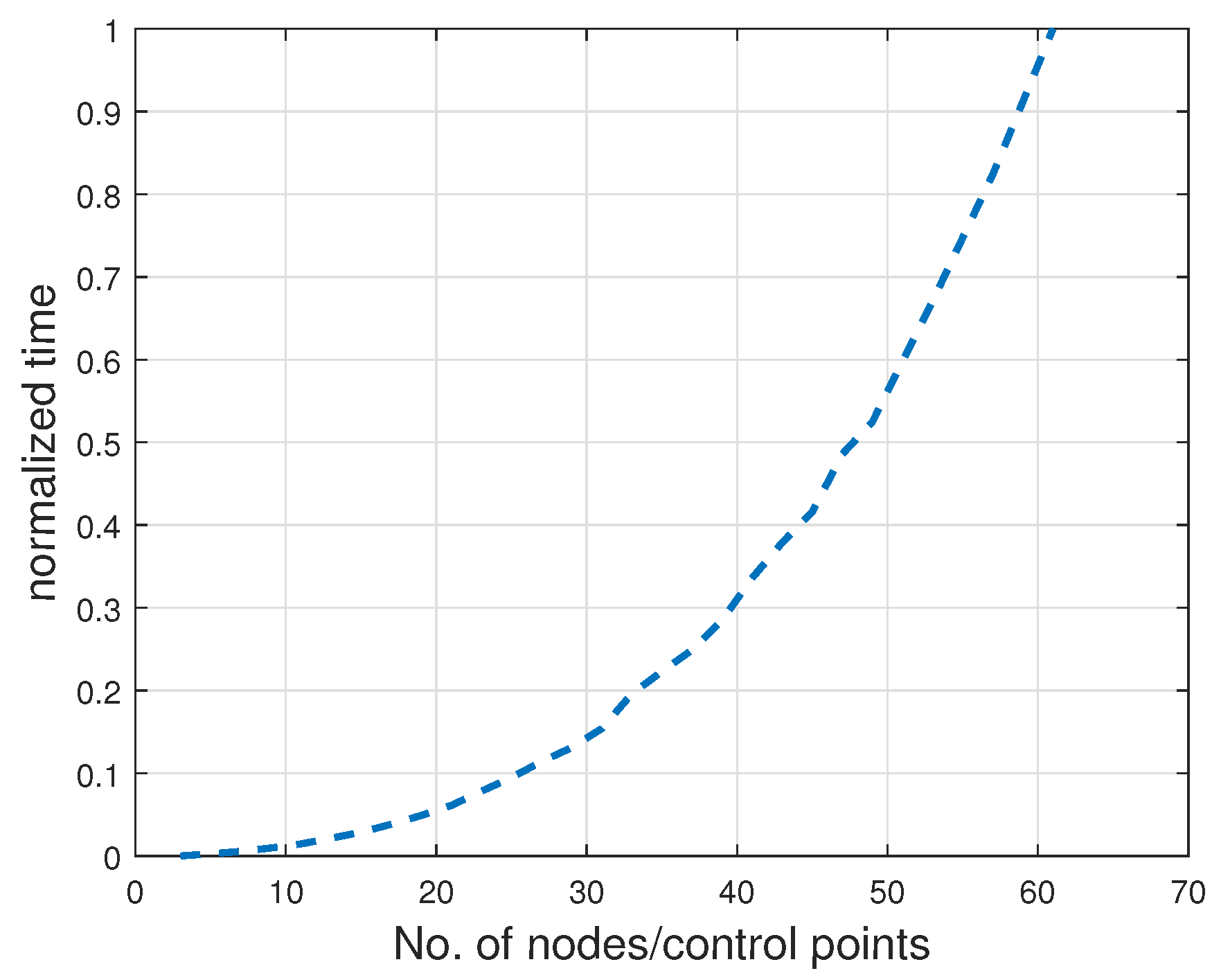
| Method | DOFs | Normalized Time |
|---|---|---|
| FEM (h-refinement, , p = 2) | 61 | 1.0000 |
| NURBS (h-refinement, , p = 2) | 33 | 0.1962 |
| NURBS (p-refinement, ) | 21 | 0.0609 |
| NURBS (k-refinement, ) | 10 | 0.0120 |
| SEM (p-refinement, GLL) | 21 | 0.0609 |
| SEM (p-refinement, CGL) | 21 | 0.0609 |
| p-FEM (p-refinement) | 21 | 0.0609 |
| FEM (p-refinement, equidistant) | 21 | 0.0609 |
| C11 | C12 | C13 | C22 | C23 | C33 | C44 | C55 | C66 |
|---|---|---|---|---|---|---|---|---|
| 164.708 | 5.453 | 5.453 | 11.300 | 4.739 | 11.300 | 3.280 | 6.000 | 6.000 |
Publisher’s Note: MDPI stays neutral with regard to jurisdictional claims in published maps and institutional affiliations. |
© 2022 by the authors. Licensee MDPI, Basel, Switzerland. This article is an open access article distributed under the terms and conditions of the Creative Commons Attribution (CC BY) license (https://creativecommons.org/licenses/by/4.0/).
Share and Cite
Mirzaee Kakhki, E.; Rezaeepazhand, J.; Duvigneau, F.; Pahlavan, L.; Makvandi, R.; Juhre, D.; Moavenian, M.; Eisenträger, S. On the Use of High-Order Shape Functions in the SAFE Method and Their Performance in Wave Propagation Problems. Math. Comput. Appl. 2022, 27, 63. https://doi.org/10.3390/mca27040063
Mirzaee Kakhki E, Rezaeepazhand J, Duvigneau F, Pahlavan L, Makvandi R, Juhre D, Moavenian M, Eisenträger S. On the Use of High-Order Shape Functions in the SAFE Method and Their Performance in Wave Propagation Problems. Mathematical and Computational Applications. 2022; 27(4):63. https://doi.org/10.3390/mca27040063
Chicago/Turabian StyleMirzaee Kakhki, Elyas, Jalil Rezaeepazhand, Fabian Duvigneau, Lotfollah Pahlavan, Resam Makvandi, Daniel Juhre, Majid Moavenian, and Sascha Eisenträger. 2022. "On the Use of High-Order Shape Functions in the SAFE Method and Their Performance in Wave Propagation Problems" Mathematical and Computational Applications 27, no. 4: 63. https://doi.org/10.3390/mca27040063
APA StyleMirzaee Kakhki, E., Rezaeepazhand, J., Duvigneau, F., Pahlavan, L., Makvandi, R., Juhre, D., Moavenian, M., & Eisenträger, S. (2022). On the Use of High-Order Shape Functions in the SAFE Method and Their Performance in Wave Propagation Problems. Mathematical and Computational Applications, 27(4), 63. https://doi.org/10.3390/mca27040063