Symbolic Computation Applied to Cauchy Type Singular Integrals

Abstract

The development of operator theory is stimulated by the need to solve problems emerging from several fields in mathematics and physics. At the present time, this theory has wide applications in the study of non-linear differential equations, in linear transport theory, in the theory of diffraction of acoustic and electromagnetic waves, in the theory of scattering and of inverse scattering, among others. In our work, we use the computer algebra system Mathematica to implement, for the first time on a computer, analytical algorithms developed by us and others within operator theory. The main goal of this paper is to present new operator theory algorithms related to Cauchy type singular integrals, defined in the unit circle. The design of these algorithms was focused on the possibility of implementing on a computer all the extensive symbolic and numeric calculations present in the algorithms. Several nontrivial examples computed with the algorithms are presented. The corresponding source code of the algorithms has been made available as a supplement to the online edition of this article.

1. Introduction

In recent years, several software applications with extensive capabilities of symbolic computation were made available to the general public. These applications, known as computer algebra systems (CAS), allow the delegation to a computer of all, or a significant part, of the symbolic and numeric calculations present in many mathematical algorithms.

In our work, we use the computer algebra system Mathematica (Wolfram Mathematica is a symbolic mathematical computation program, conceived by Stephen Wolfram, used in many scientific, engineering and computing fields) to implement for the first time on a computer analytical algorithms developed by us and others within the operator theory. The design of our algorithms is focused on the possibility of implementing on a computer all, or a significant part, of the extensive symbolic and numeric calculations present in the analytical algorithms. The methods developed rely on innovative techniques of operator theory and have a potential for extension to more complex and general problems. By implementing these methods on a computer, new tools are created to explore that same potential, making the results of lengthy and complex calculations available in a simple way to researchers in different areas. In the last years, we designed and/or implemented calculation techniques to compute singular integrals, analytical algorithms for solving integral equations, to study the spectrum and the kernel of several special classes of singular integral operators and to factorize functions (see, for instance [1,2,3,4,5]).

The main goal of this paper is to present new operator theory algorithms related to Cauchy type singular integrals, defined in the unit circle. All the algorithms were implemented using the symbolic computation capabilities of the computer algebra system Mathematica.

Singular integrals are classic mathematical objects with a vast array of applications in the main scientific research areas, and the importance of their study is globally acknowledged. There are several numerical algorithms and approximation methods for evaluating some classes of singular integrals. There exist also several analytical techniques that allow the exact computation of particular classes of singular integrals. However, the [SInt] and [SIntAFact] algorithms [2] are the only analytical algorithms, to our knowledge, written and implemented for computing Cauchy type singular integrals with general functions, defined in the unit circle. Although the [SInt] algorithm was designed to be efficient for a wide class of singular integrals, it can be improved in terms of implementation. For instance, the version described and made available in [2] does not identify whether a given function has poles in the unit circle or if the user inputs non-valid functions, nor can it work with the generality of fifth degree or higher polynomials.

In this paper, we present an improved and fully efficient version of the algorithm, the [SInt]${}_{2.0}$ algorithm, designed with the Root object concept (to represent solutions to one-variable algebraic equations) available in Wolfram Mathematica. This conception of an improved version became possible after the design of the [ASPPlusPMinus] algorithm, created for the rational case, which also calculates the projections associated with the integral of type Cauchy considered in [2], even in cases involving polynomials of the fifth degree or higher. The output provided by these algorithms can be used for several other algorithms to solve singular integral equations, to factorize functions, to compute the dimension of the kernel of some classes of singular integrals and to study the spectra of some operators. Furthermore, since the majority of the concepts and results established for the unit circle within operator theory can be generalized for the real line, we are trying to make the several necessary adaptations in analytical and implementation terms so that the creation of new algorithms that use functions defined in the real line becomes possible. We believe that it will also be possible to extend the methods described in this article to other classes of singular integrals of the Cauchy type, such as those studied in [1,5,6,7,8], at least for the rational case.

The paper is organized as follows: Section 2 contains some basic concepts within Cauchy singular integral operators and a brief description of the [SInt] algorithm. The section also contains the description of algorithms that compute the roots (in exact and approximate forms) of a polynomial function and/or identify the location (regarding the unit circle) of elements that belong to a list of complex numbers and that can be integrated into new operator algorithms. Section 3 is dedicated to the [SInt]${}_{2.0}$ algorithm and to the description of a new operator theory algorithm that uses the algorithms presented in Section 2.3 and Section 2.4. Section 2 and Section 3 contains several nontrivial examples computed with the algorithms. The last section is dedicated to some final comments.

The corresponding source code of the algorithms has been made available as a Supplementary Material to the online edition of this article.

2. Materials and Methods

This section contains some basic concepts within Cauchy singular integral operators and a brief description of the [SInt] algorithm [2]. Some algorithms that compute the roots (in exact and approximate forms) of a polynomial function and/or identify the location (regarding the unit circle) of elements that belong to a given list of complex numbers are also presented.

2.1. Basic Concepts

Let $\mathbb{T}$ denote the unit circle in the complex plane. Let ${\mathbb{T}}_{+}$ and ${\mathbb{T}}_{-}$ denote the open unit disk and the exterior region of the unit circle (∞ included), respectively. As usual, $L_{\infty }\left(\mathbb{T}\right)$ denotes the space of all essentially bounded functions defined on $\mathbb{T}$ and $H_{\infty }\left(\mathbb{T}\right)$ the class of all bounded and analytic functions in ${\mathbb{T}}_{+}$. Let $\mathcal{R}\left(\mathbb{T}\right)$ be the algebra of rational functions without poles on $\mathbb{T}$ and ${\mathcal{R}}_{\pm }\left(\mathbb{T}\right)$ the subsets of $\mathcal{R}\left(\mathbb{T}\right)$ whose elements have no poles in ${\mathbb{T}}_{\pm }$, respectively.

The study of singular integral operators has applications in different research areas, such as the theory of diffraction of acoustic and electromagnetic waves, theory of scattering and of inverse scattering and factorization theory (see, for instance, [9,10,11,12,13,14,15,16]).

It is well known that the singular integral operator with Cauchy kernel, $S_{\mathbb{T}}$, defined almost everywhere on $\mathbb{T}$, by

$${\displaystyle S_{\mathbb{T}}\phi \left(t\right)=\frac{1}{\pi i}{\int }_{\mathbb{T}}\frac{\phi \left(\tau \right)}{\tau -t}d\tau ,t\in \mathbb{T},}$$

(1)

where the integral is understood in the sense of its principal value, represents a bounded linear operator in the Lebesgue space $L_2\left(\mathbb{T}\right)$. In addition, $S_{\mathbb{T}}$ is a selfadjoint and unitary operator in $L_2\left(\mathbb{T}\right)$ [17]. Thus, we can associate with $S_{\mathbb{T}}$ two complementary Cauchy projection operators

$$P_{\pm }=(I\pm S_{\mathbb{T}})/2,$$

(2)

where I represents the identity operator.

The projectors (2) allow us to decompose the algebra $\mathcal{R}\left(\mathbb{T}\right)$ in the topological direct sum

$$\mathcal{R}\left(\mathbb{T}\right)={\mathcal{R}}_{+}\left(\mathbb{T}\right)\oplus {\mathcal{R}}_{-}^0\left(\mathbb{T}\right)$$

(3)

where ${\mathcal{R}}_{+}\left(\mathbb{T}\right)=P_{+}\mathcal{R}\left(\mathbb{T}\right)$ and ${\mathcal{R}}_{-}^0\left(\mathbb{T}\right)=P_{-}\mathcal{R}\left(\mathbb{T}\right)$. We also have ${\mathcal{R}}_{-}\left(\mathbb{T}\right)={\mathcal{R}}_{-}^0\left(\mathbb{T}\right)\oplus \mathbb{C}$.

2.2. [SInt] Algorithm

There exist several numerical algorithms and approximation methods for evaluating some classes of singular integrals. There are also several analytical techniques that allow the exact computation of singular integrals for particular cases. However, the [SInt] (the corresponding source code of [SInt] is available in the online version of [2]) and [SIntAFact] algorithms [2] are the only analytical algorithms, to our knowledge, designed and implemented for computing singular integrals with general essentially bounded functions defined on the unit circle. Both algorithms were implemented using the numeric and symbolic computation capabilities of the computer algebra system Mathematica. In particular, the implementation of the [SInt] algorithm makes the results of lengthy and complex calculations available in a simple way to researchers of different areas.

The [SInt] algorithm computes (1) when we can represent the function $\phi$ as

$$\phi \left(t\right)=r\left(t\right)[x_{+}\left(t\right)+y_{-}\left(t\right)],$$

(4)

where $x_{+},\overline{y_{-}}\in H_{\infty }\left(\mathbb{T}\right)$ and $r\in \mathcal{R}\left(\mathbb{T}\right)$.

The algorithm extensively uses the properties of the projection operators (2) that emerge when those operators are applied to functions in $H_{\infty }\left(\mathbb{T}\right)$ (e.g., $x_{+}$) and in $\overline{H_{\infty }\left(\mathbb{T}\right)}$, (e.g., $y_{-}$). [SInt] also explores the rationality of $r\left(t\right)$ for reducing all possible situations to a few basic cases. After the decomposition of the rational function r(t) in elementary fractions, the singular integrals are computed using formulas described in [2].

The [SInt] algorithm can be applied to particular functions $x_{+}\left(t\right)$ and $y_{-}\left(t\right)$, or it can compute the closed form of (1) as a general expression in $x_{+}\left(t\right)$ and $y_{-}\left(t\right)$.

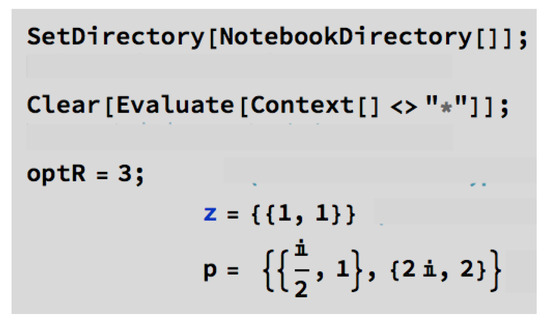
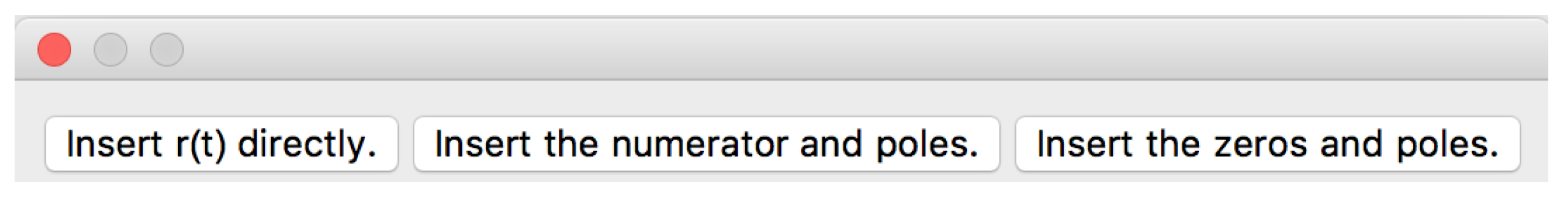
There are three options to insert the rational function $r\left(t\right)$:

• Input $r\left(t\right)$ directly;
• Input the numerator and the poles and multiplicities;
• Input zeros, poles and multiplicities.

It is important to note that in the [SInt] algorithm, it is entirely the user’s responsibility to introduce a function r that belong to $\mathcal{R}\left(\mathbb{T}\right)$, a function $x_{+}$ in $H_{\infty }\left(\mathbb{T}\right)$ and a function $y_{-}$ whose conjugate is in $H_{\infty }\left(\mathbb{T}\right)$. If a non-valid input is considered, [SInt] outputs an error. Furthermore, since the poles of r are crucial information for this calculation technique, in the case of Option 1, or if a particular function $x_{+}$ or $y_{-}$ is considered, the success of the [SInt] algorithm is dependent on the possibility of finding those poles by solving a polynomial equation. For instance, if a rational function r is introduced with fifth degree or higher polynomials, the algorithm gives, most of the time, an incorrect output (since it cannot apply the properties of the projectors).

2.2.1. [SInt] Algorithm Examples

We now present some examples of nontrivial singular integrals computed with the source code of [SInt], which is available in the online version of [2]. For each input of functions $r\left(t\right)$, $x_{+}\left(t\right)$, and $y_{-}\left(t\right)$, the [SInt] algorithm computes the singular integrals $S_{\mathbb{T}}X\left(t\right)$ and $S_{\mathbb{T}}Y\left(t\right)$, for $X\left(t\right)=r\left(t\right)x_{+}\left(t\right)$ and $Y\left(t\right)=r\left(t\right)y_{-}\left(t\right)$.

It should be noted that it is up to the user to introduce valid r, $x_{+}$ and $y_{-}$ functions.

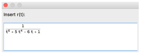
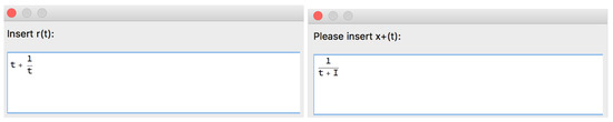
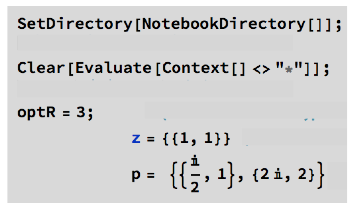
Example 1.

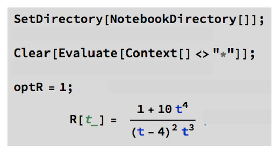
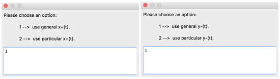
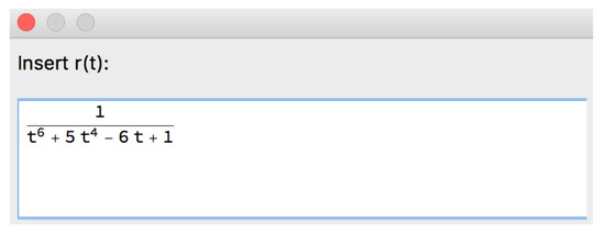
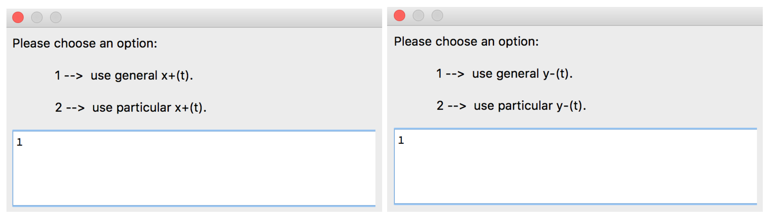
Let us use Option 1 to input the rational function r (Figure 1). Let us consider a general expression for the function $x_{+}$ and $y_{-}\left(t\right)=t^{-k}$ (Figure 2).

Figure 1. Part of the structure of the [SInt] algorithm corresponding to the Option 1 to input r.

Figure 2. Part of the structure of the [SInt] algorithm corresponding to the Input of $x_{+}$ and $y_{-}$.

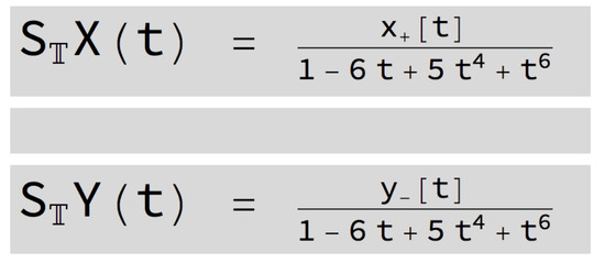
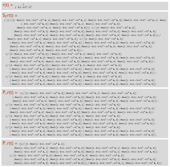
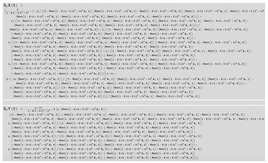
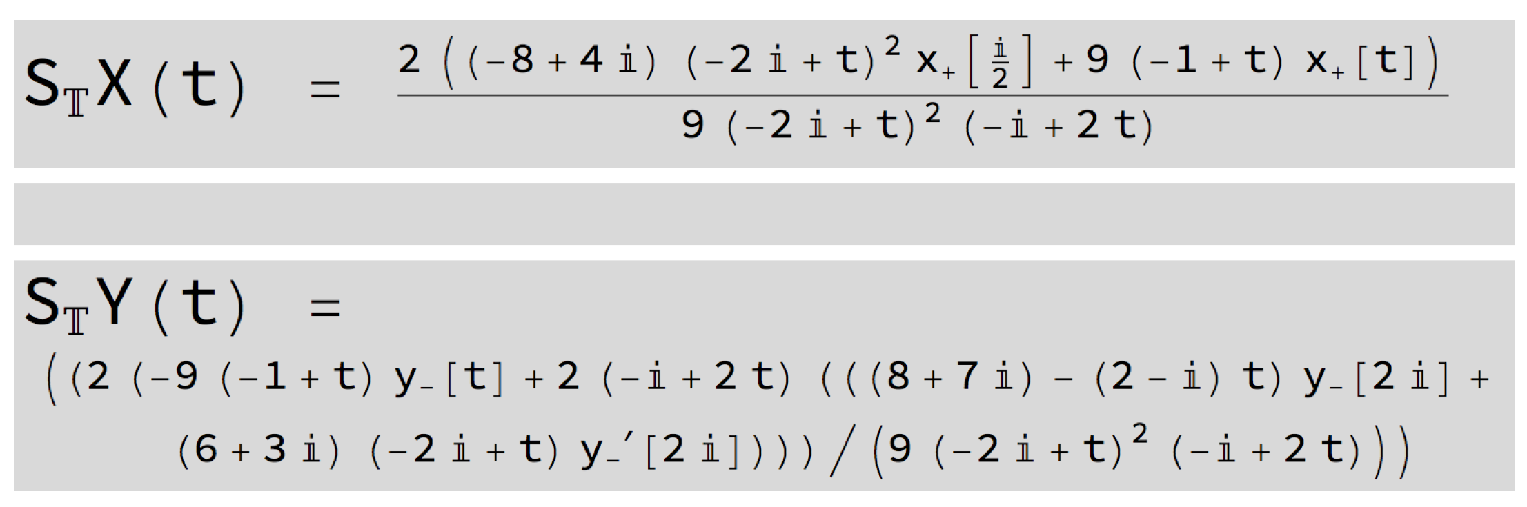
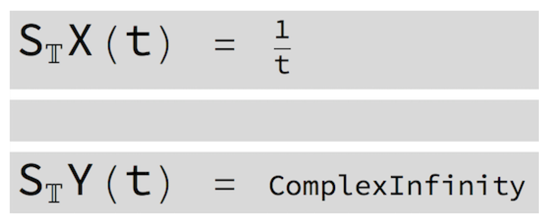
The [SInt] algorithm gives the singular integrals presented in Figure 3.

Figure 3. Output given by the [SInt] algorithm.

Remark 1.

In this example, we should interpret that the [SInt] algorithm considers $k⩾0$, taking into account that in the input (which allows you to include arbitrary constants), $\overline{y_{-}}\in H_{\infty }\left(\mathbb{T}\right)$.

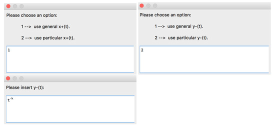
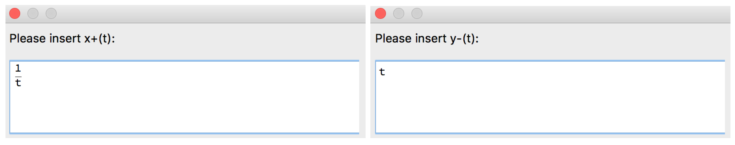
Example 2.

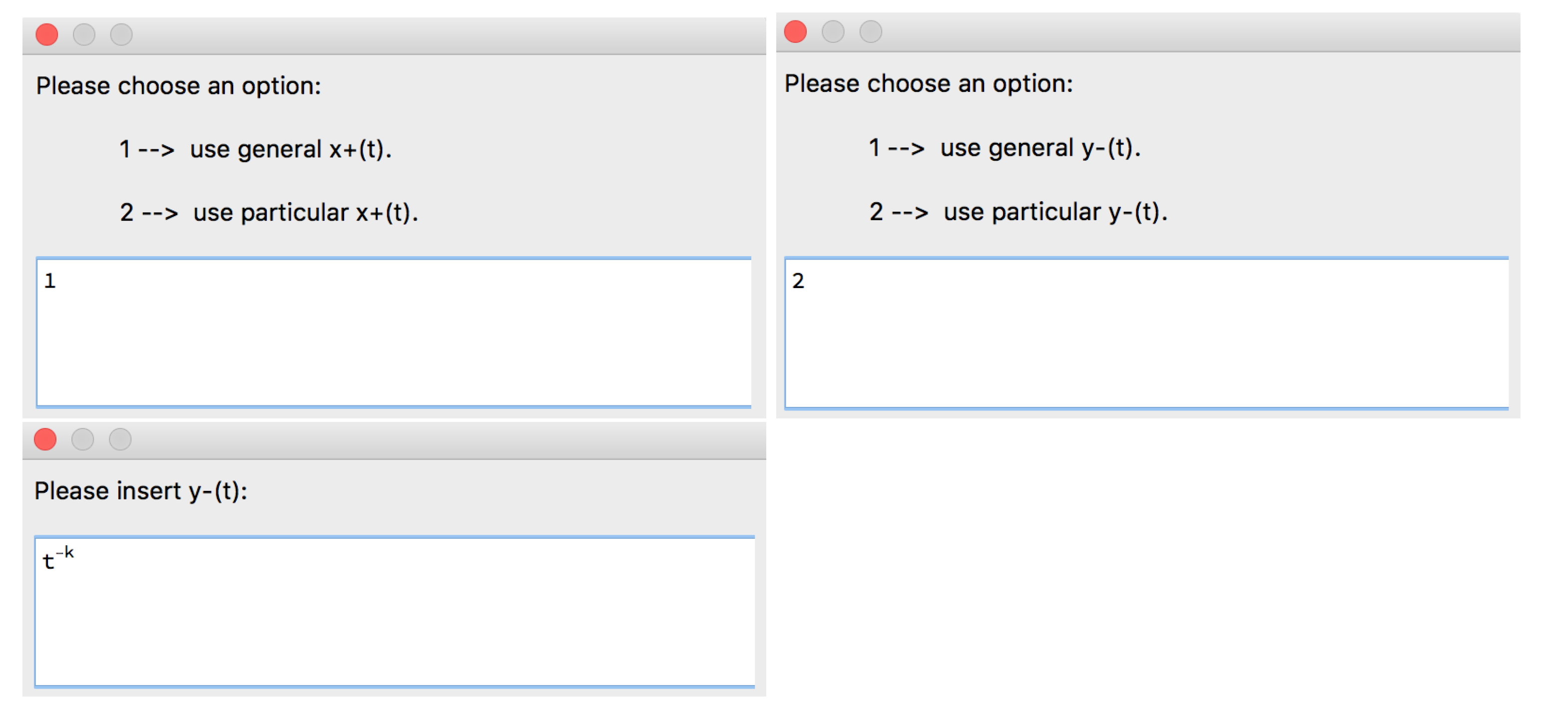
Let us use Option 2 to input the rational function r (Figure 4). Let us consider a general expression for the function $y_{-}$ and $x_{+}\left(t\right)={(t-i)}^3$ (Figure 5).

Figure 4. Part of the structure of the [SInt] algorithm corresponding to the Option 2 to input r.

Figure 5. Part of the structure of the [SInt] algorithm corresponding to the input of $x_{+}$ and $y_{-}$.

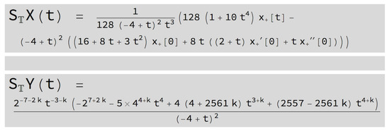
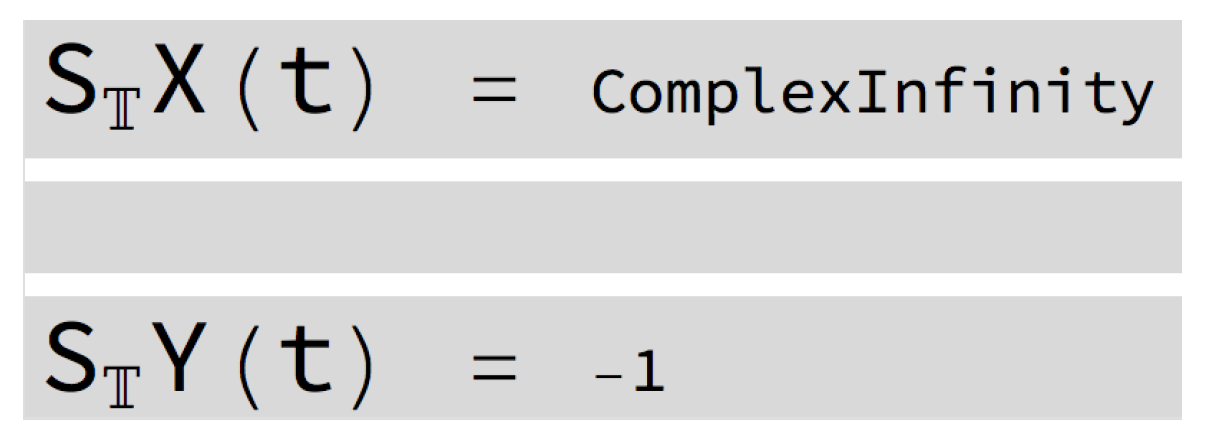
The [SInt] algorithm gives the singular integrals presented in Figure 6.

Figure 6. Output given by the [SInt] algorithm.

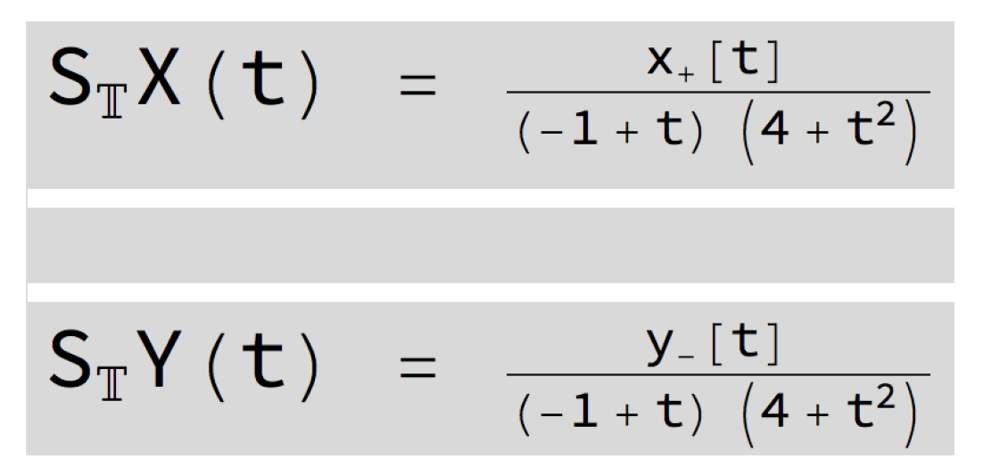
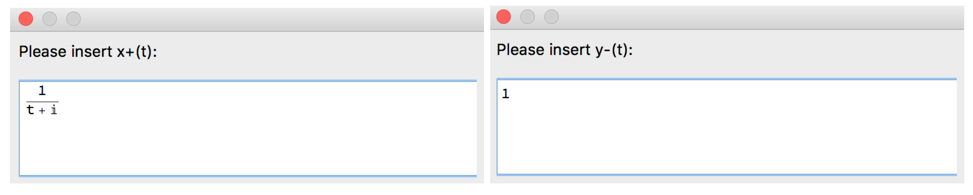
Example 3.

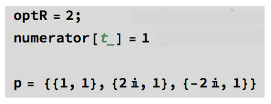
Let us use Option 3 to input the rational function r (Figure 7).

Figure 7. Part of the structure of the [SInt] algorithm corresponding to Option 3 to input r.

Let us consider a general expression for the functions $x_{+}$ and $y_{-}$ (Figure 8).

Figure 8. Part of the structure of the [SInt] algorithm corresponding to the input of $x_{+}$ and $y_{-}$.

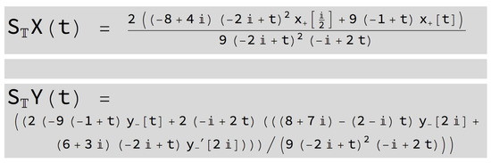
The [SInt] algorithm gives the singular integrals presented in Figure 9.

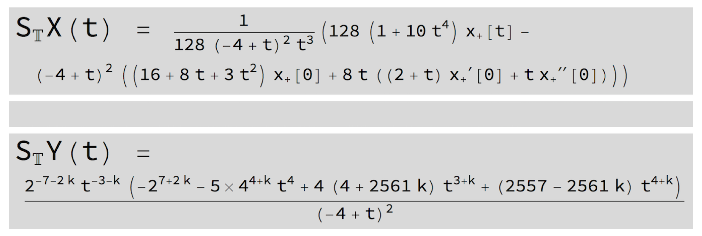
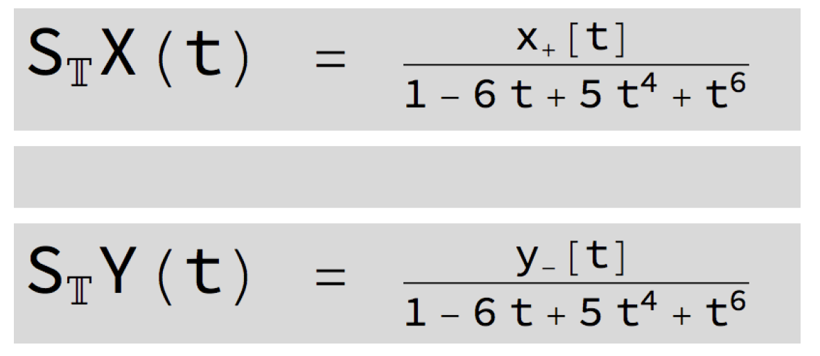
Figure 9. Output given by the [SInt] algorithm.

2.2.2. [SInt] Algorithm: Possible Improvements

Now, we present some situations not considered in the implementation of the [SInt] algorithm and that are considered in our improved version in Section 3.

• Situation 1: The [SInt] algorithm does not identify whether an inputed function has poles in $\mathbb{T}$.

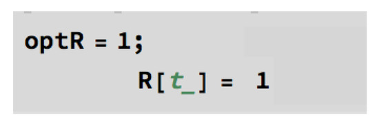
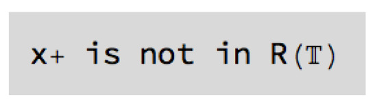
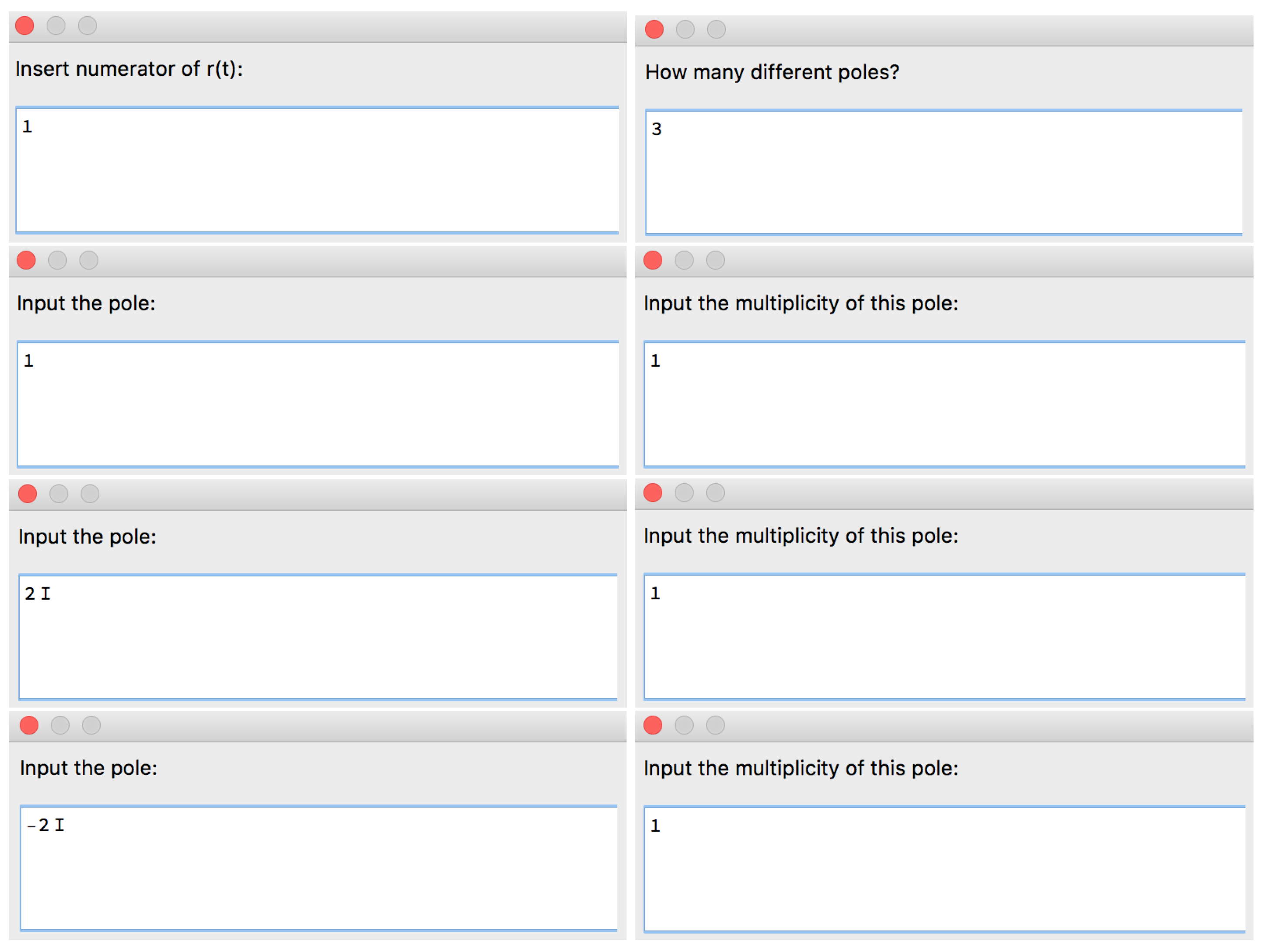
Example 4.

Let us use Option 2 to input the rational function r (Figure 10) and general expressions for the functions $x_{+}$ and $y_{-}$.

Figure 10. Part of the structure of the [SInt] algorithm corresponding to Option 2 to input r.

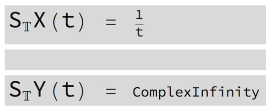
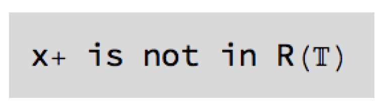
The [SInt] algorithm gives the incorrect output presented in Figure 11 since $r\notin \mathcal{R}\left(\mathbb{T}\right)$.

Figure 11. Output given by the [SInt] algorithm.

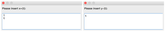
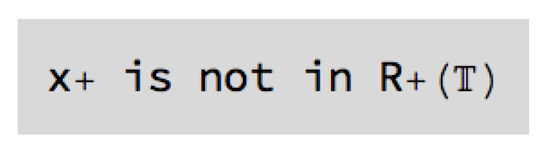
Example 5.

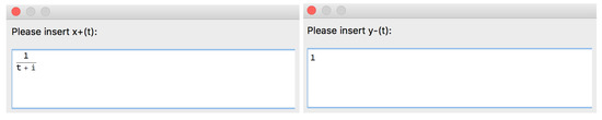
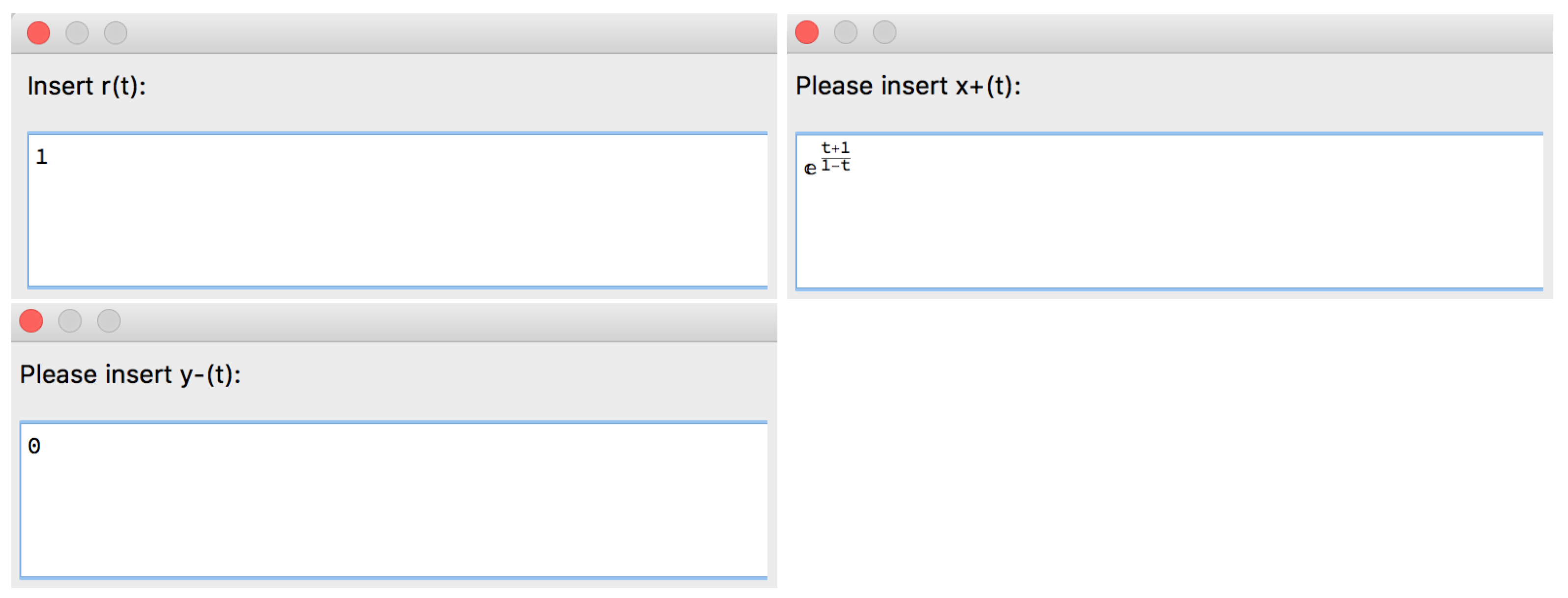
Let us use Option 1 to input the rational function r (Figure 12) and particular functions $x_{+}$ and $y_{-}$ (Figure 13)..

Figure 12. Part of the structure of the [SInt] algorithm corresponding to Option 1 to input r.

Figure 13. Part of the structure of the [SInt] algorithm corresponding to the input of $x_{+}$ and $y_{-}$.

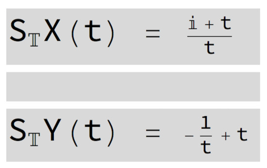
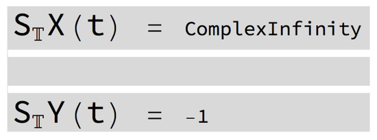
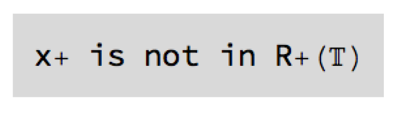
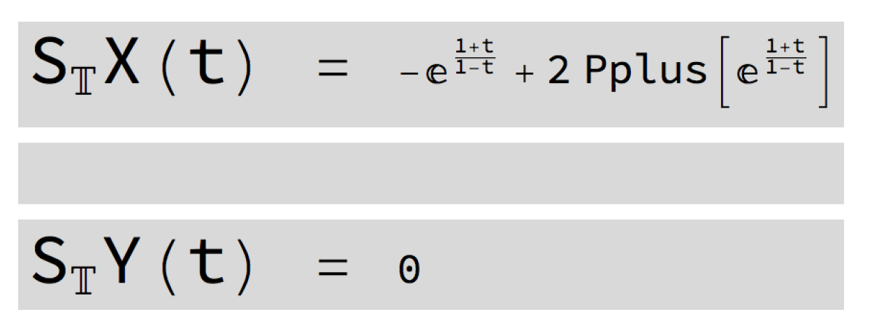
The [SInt] algorithm gives the incorrect output presented in Figure 14 since $x_{+}\notin \mathcal{R}\left(\mathbb{T}\right)$.

Figure 14. Output given by the [SInt] algorithm.

Something similar would happen for an inputed function $y_{-}$ with one pole on $\mathbb{T}$.

Remark 2.

Situation 1 is resolved in the improved version of the algorithm, described in Section 3.

• Situation 2: The [SInt] algorithm does not identify whether valid functions $x_{+}$ and $y_{-}$ are inputed.

Example 6.

Let us use Option 1 to input the rational function r (Figure 15). Let us consider particular functions $x_{+}$ and $y_{-}$ (Figure 16).

Figure 15. Part of the structure of the [SInt] algorithm corresponding to the Option 1 to input r.

Figure 16. Part of the structure of the [SInt] algorithm corresponding to the Input of $x_{+}$ and $y_{-}$.

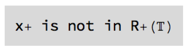
The [SInt] algorithm gives the incorrect output presented in Figure 17 since $x_{+}$ and $y_{-}$ are non-valid functions.

Figure 17. Output given by the [SInt] algorithm.

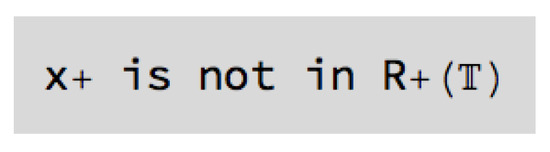
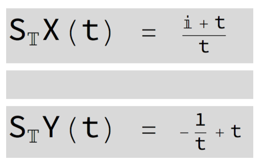
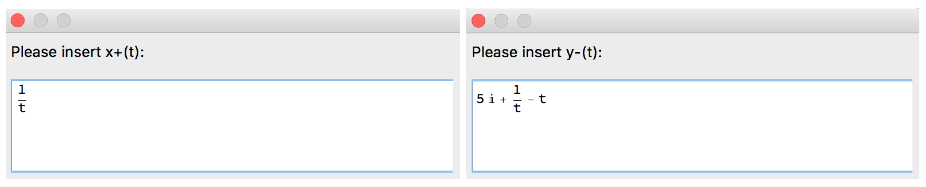
Example 7.

Let us use Option 1 to input the rational function r (Figure 18).

Figure 18. Part of the structure of the [SInt] algorithm corresponding to Option 1 to input r.

Let us consider particular functions $x_{+}$ and $y_{-}$ (Figure 19). The [SInt] algorithm gives the incorrect output presented in Figure 20 since $x_{+}$ and $y_{-}$ are non-valid functions.

Figure 19. Part of the structure of the [SInt] algorithm corresponding to the input of $x_{+}$ and $y_{-}$.

Figure 20. Output given by the [SInt] algorithm.

Remark 3.

The Situation 2 is resolved, for the rational case, in the [SInt]${}_{2.0}$ algorithm.

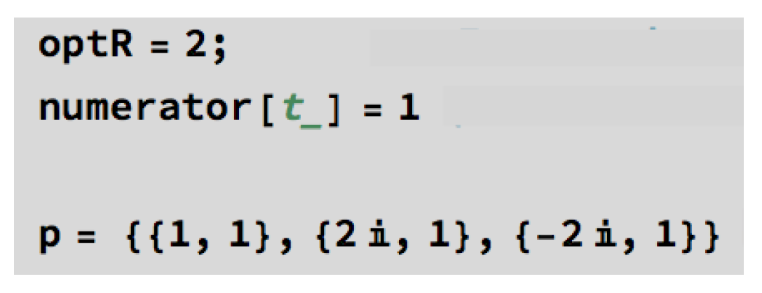
• Situation 3: The [SInt] algorithm is not always efficient with a fifth degree or higher polynomial input.

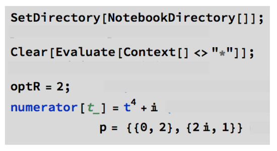
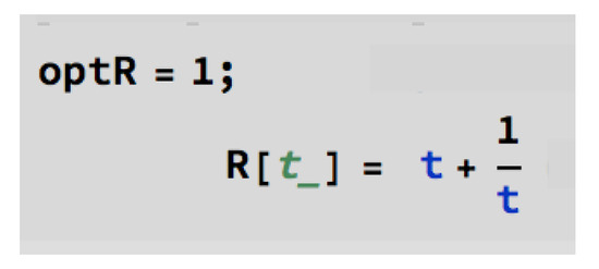
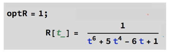
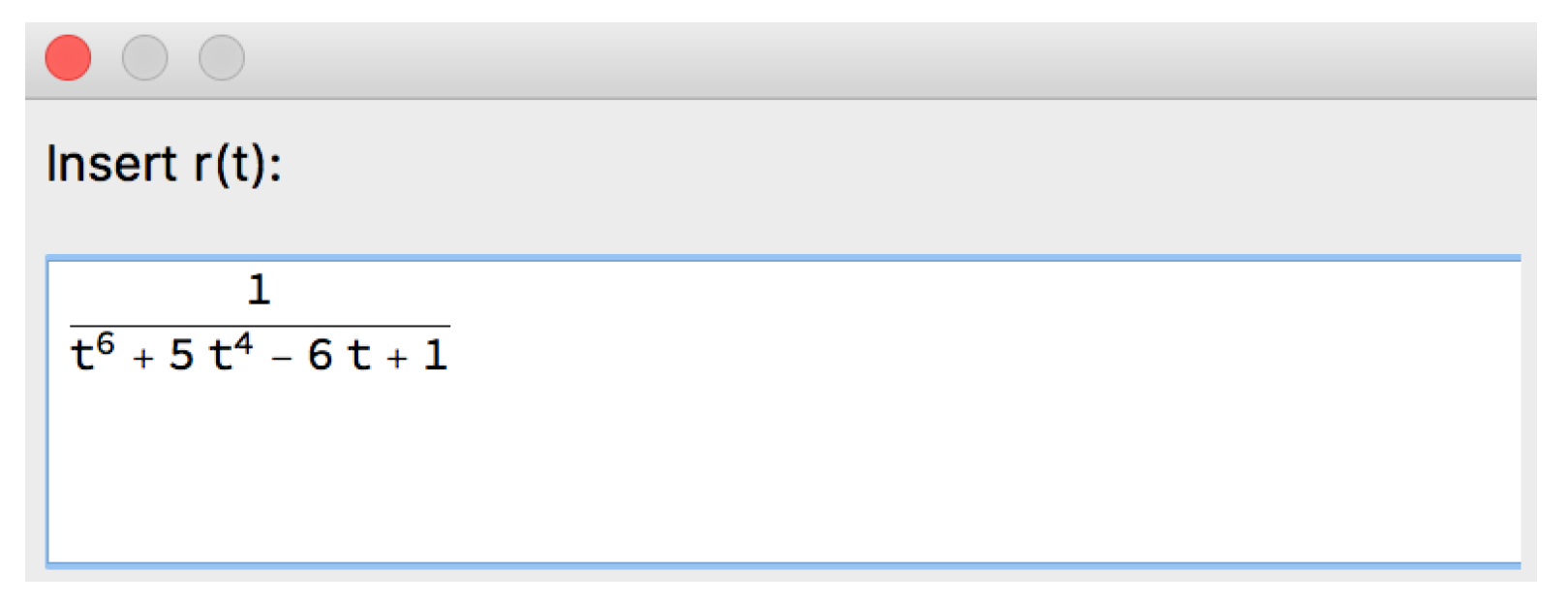
Example 8.

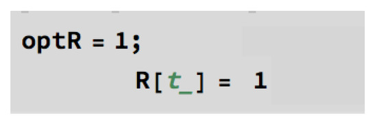
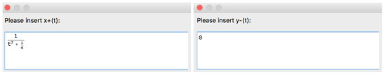
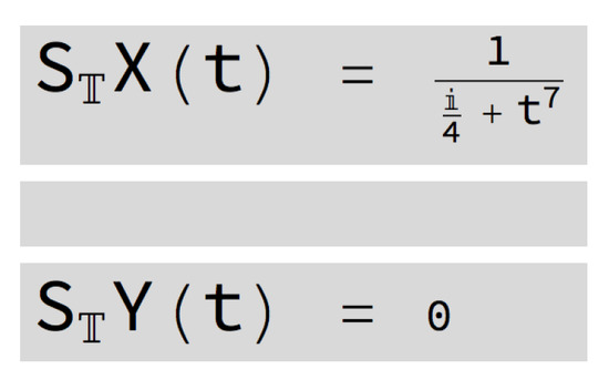
Let us use Option 1 to input the rational function r (Figure 21). Let us consider particular functions $x_{+}$ and $y_{-}$ presented in Figure 22.

Figure 21. Part of the structure of the [SInt] algorithm corresponding to Option 1 to input r.

Figure 22. Part of the structure of the [SInt] algorithm corresponding to the input of $x_{+}$ and $y_{-}$.

The [SInt] algorithm gives the incorrect output presented in Figure 23 since it cannot identify the poles of the function $x_{+}$ and assumes that $x_{+}\in H_{\infty }\left(\mathbb{T}\right)$ (in this case, $x_{+}\in {\mathcal{R}}_{-}^0\left(\mathbb{T}\right)$, that is, $x_{+}$ is an non-valid input).

Figure 23. Output given by the [SInt] algorithm.

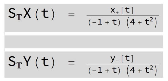
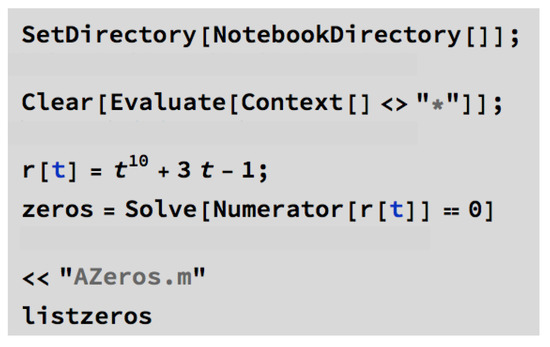
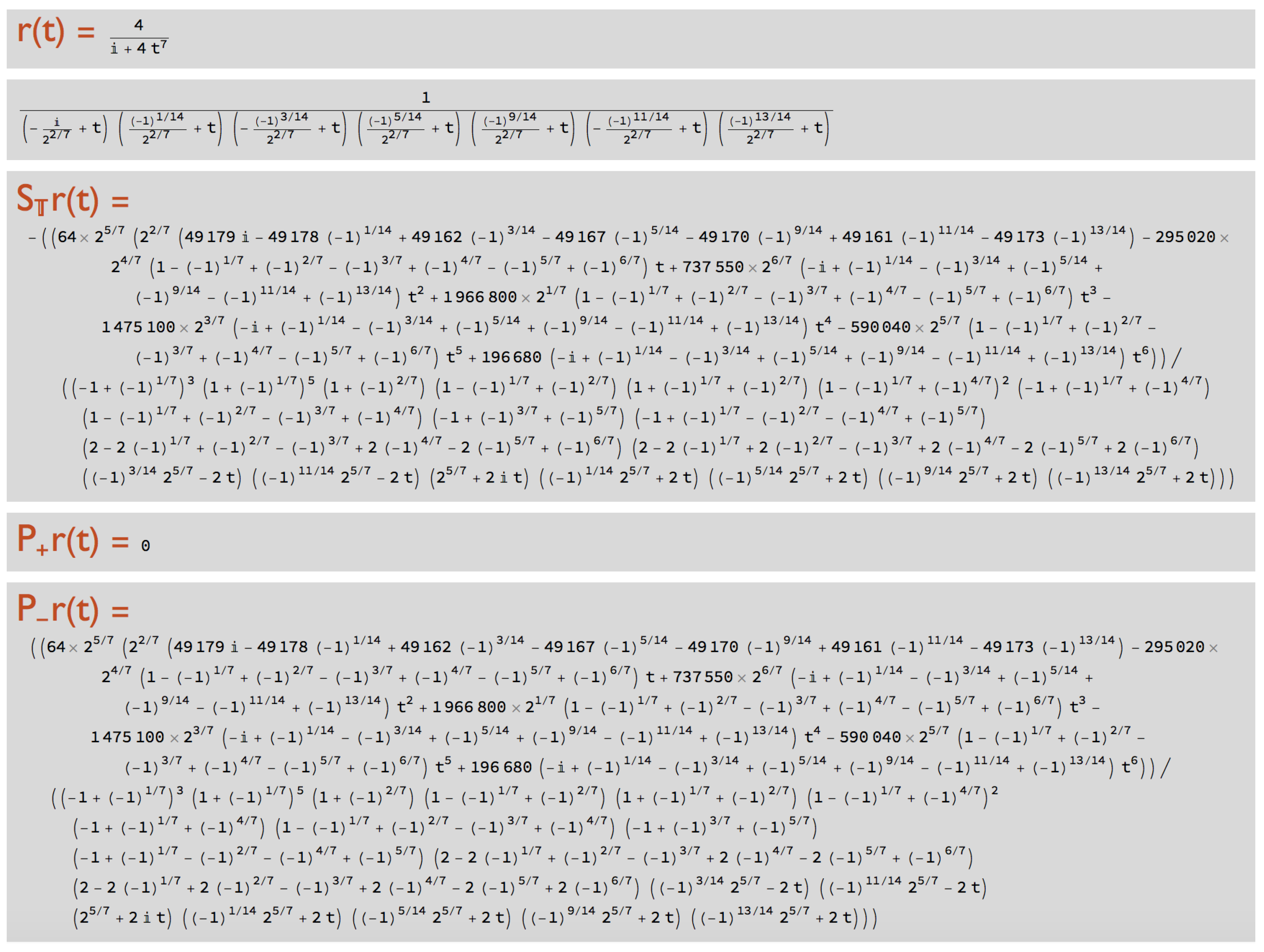
Example 9.

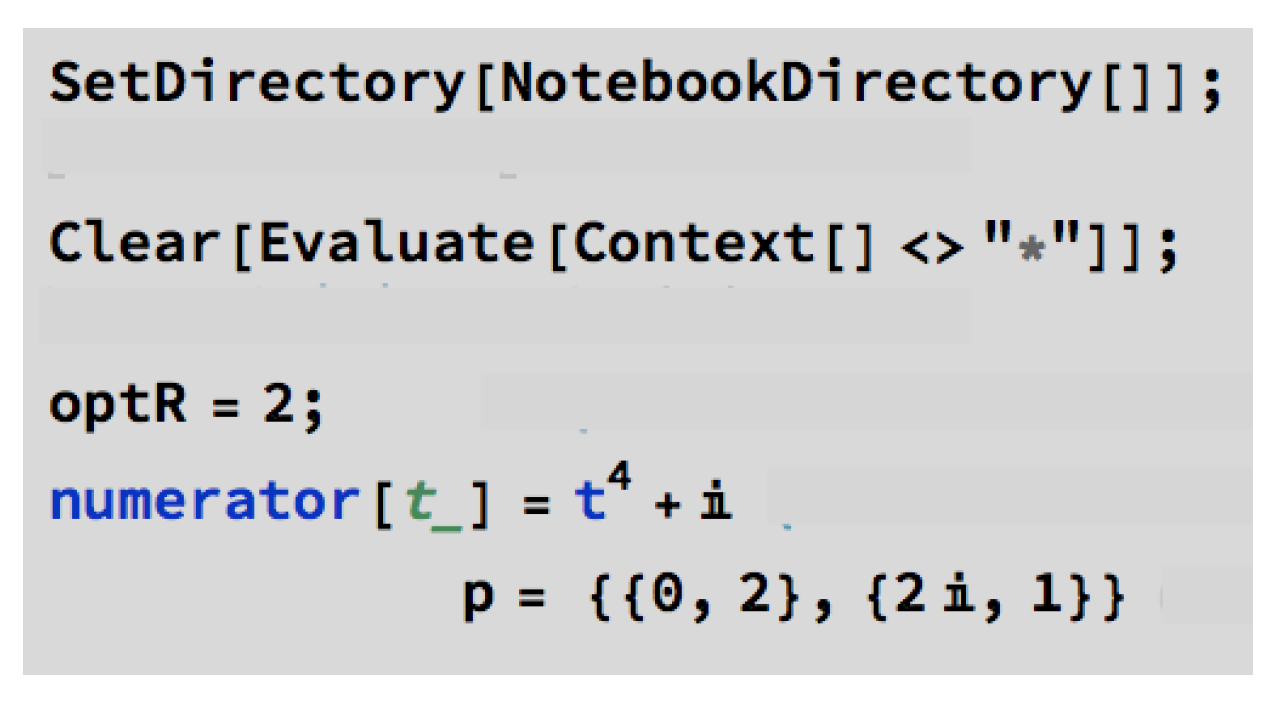
Let us use Option 1 to input the rational function r (Figure 24).

Figure 24. Part of the structure of the [SInt] algorithm corresponding to Option 1 to input r.

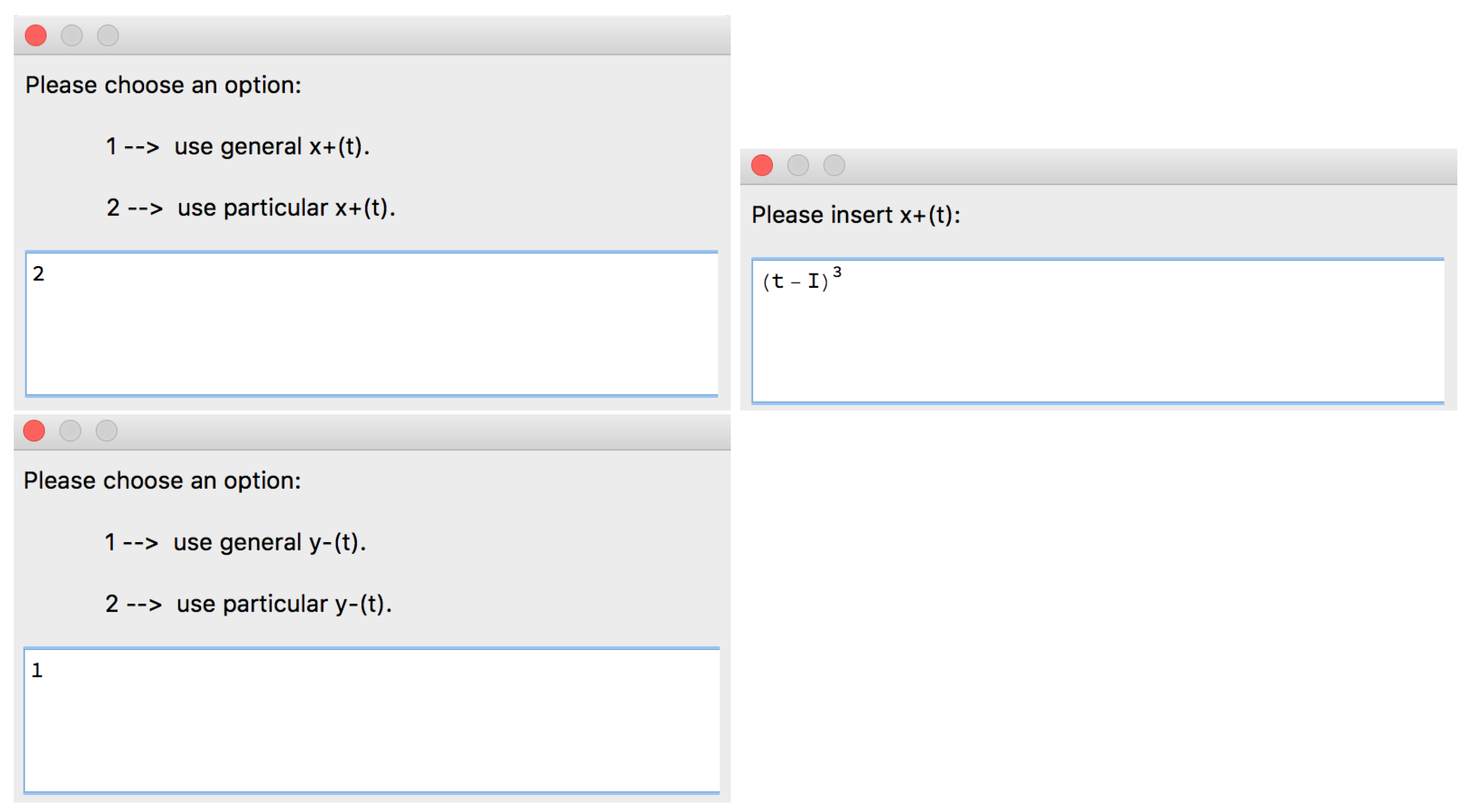
Let us consider a general expression for the functions $x_{+}$ and $y_{-}$ (Figure 25).

Figure 25. Part of the structure of the [SInt] algorithm corresponding to the input of $x_{+}$ and $y_{-}$.

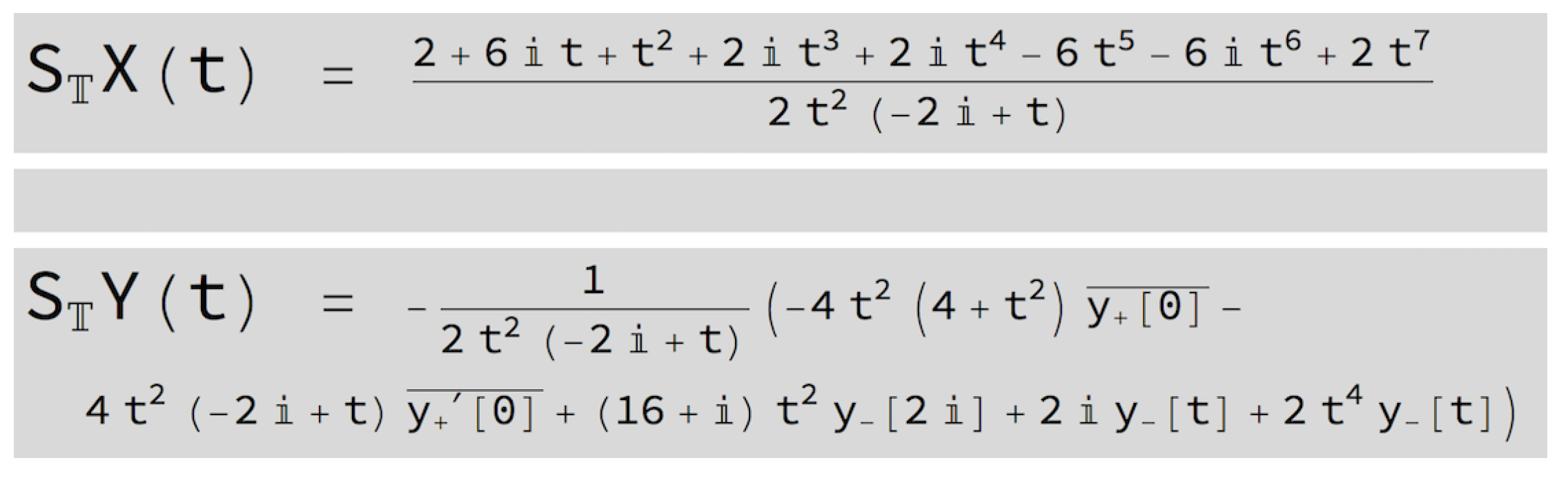
The [SInt] algorithm gives the incorrect output presented in Figure 26 since, as it cannot identify the poles of the rational function r, it does not know where they are in the complex plane (relative to $\mathbb{T}$, ${\mathbb{T}}_{+}$, and ${\mathbb{T}}_{-}$).

Figure 26. Output given by the [SInt] algorithm.

Remark 4.

Situation 3 is also resolved in the [SInt]${}_{2.0}$ algorithm, described in Section 3.

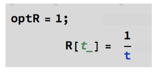
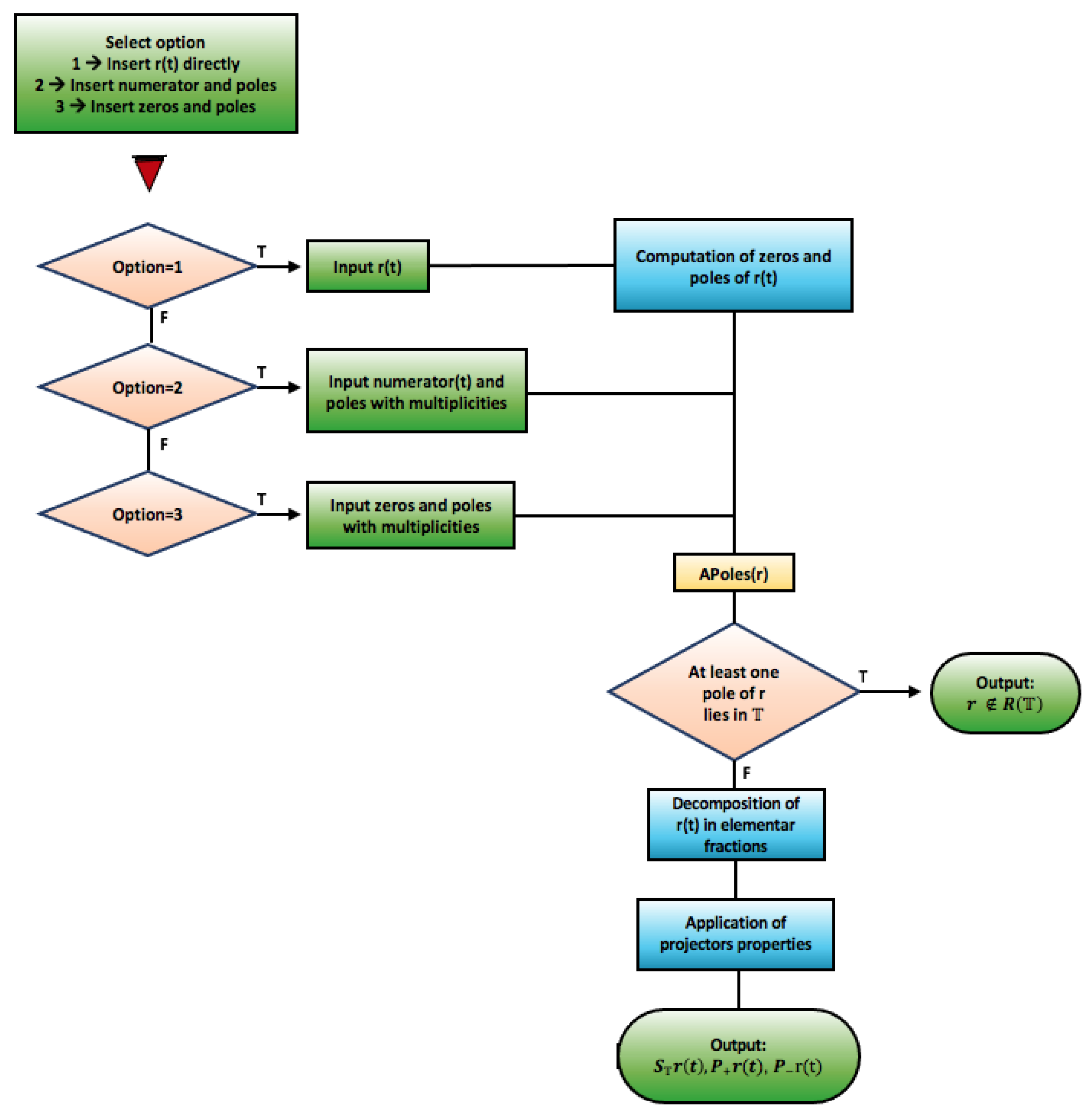
2.3. [ARoots] Algorithm

This subsection is dedicated to the formal description of the [ARoots] algorithm. This algorithm identifies, after calculating the roots of a polynomial $p\left(t\right)$, the location of the roots relative to $\mathbb{T}$, ${\mathbb{T}}_{+}$, and ${\mathbb{T}}_{-}$. It is also possible to ask for an approximate value of a desired root.

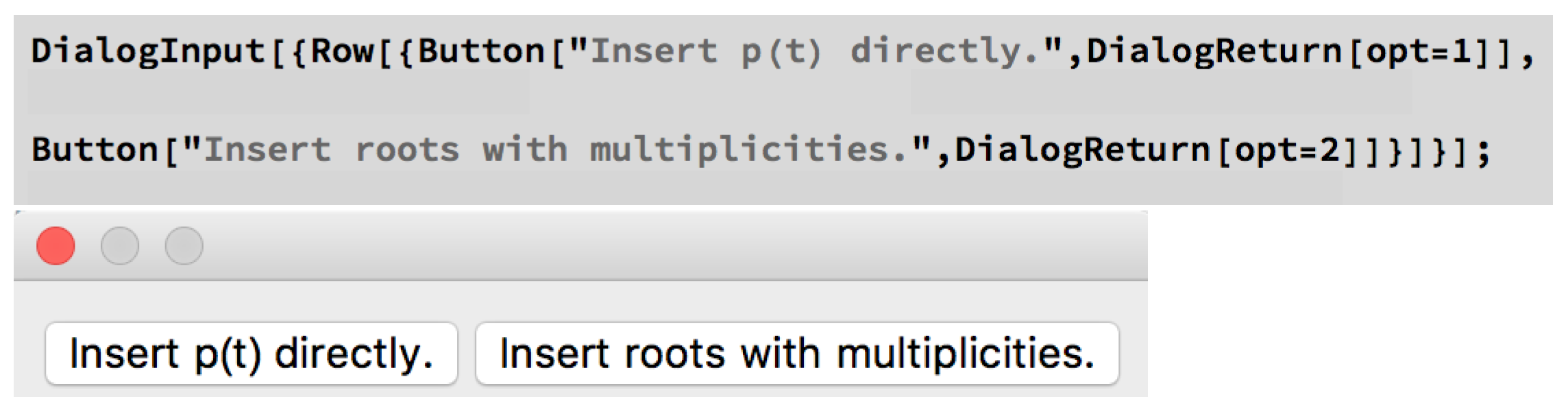
There are two options to insert the polynomial $p\left(t\right)$ (see Figure 27).

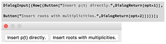
Figure 27. Part of the code structure of the [ARoot] algorithm responsible for the input options for the polynomial p.

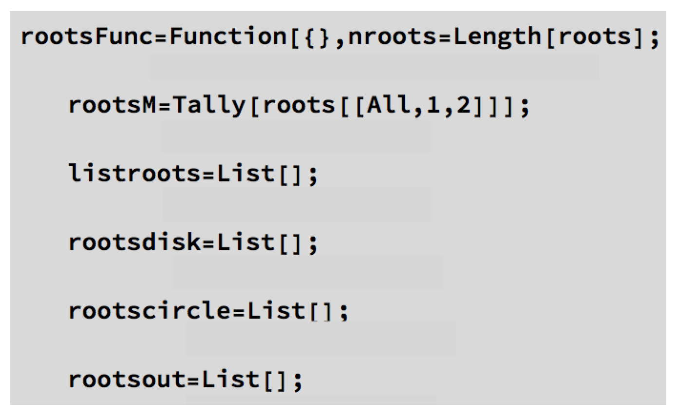
The analysis of the code and flowchart of the [ARoots] algorithm reveals that one of the essential steps is the use of the Root object concept (see Figure 28), which allows a precise analysis of the absolute value of the roots (see Figure 29).

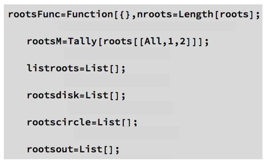
Figure 28. Part of the code structure of the [ARoot] algorithm responsible for the computation of the roots of p.

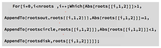
Figure 29. Part of the code structure of the [ARoots] algorithm code corresponding to the analysis of the absolute value of the roots of the inputed polynomial.

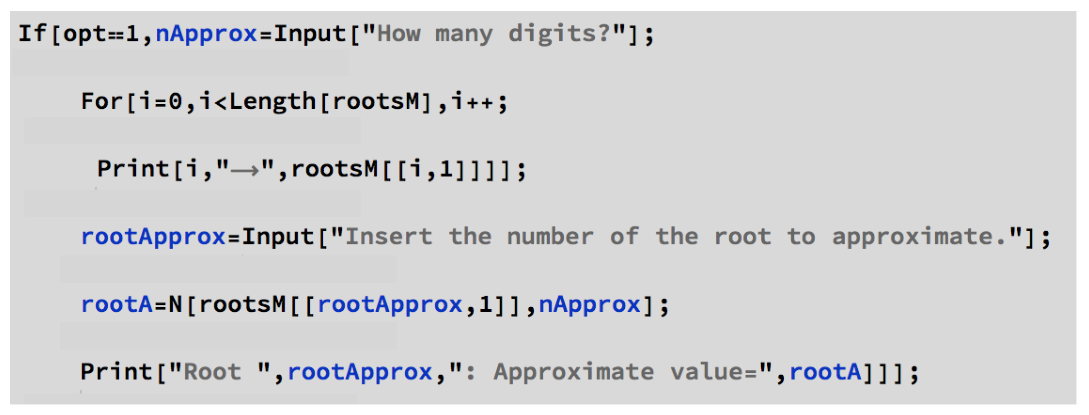
When the user uses Option 1, it is possible to ask for an approximate value of a desired root (see Figure 30).

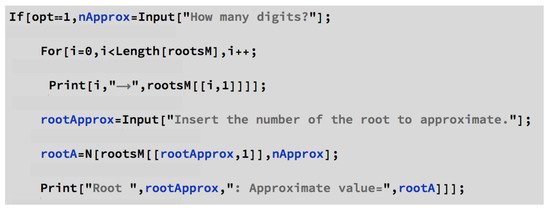
Figure 30. Part of the code structure of the [ARoots] algorithm code corresponding to the computation of an approximate value of a desired root.

Figure 31 contains the flowchart of the [ARoots] algorithm.

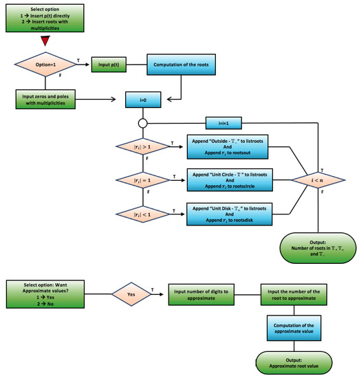
Figure 31. Flowchart of the [ARoots] algorithm.

[ARoots] Algorithm Example

Let us now present a nontrivial example computed with the [ARoots] algorithm. For each inputed polynomial p, defined in $\mathbb{T}$, the algorithm gives the number of roots in $\mathbb{T}$, ${\mathbb{T}}_{+}$, and ${\mathbb{T}}_{-}$.

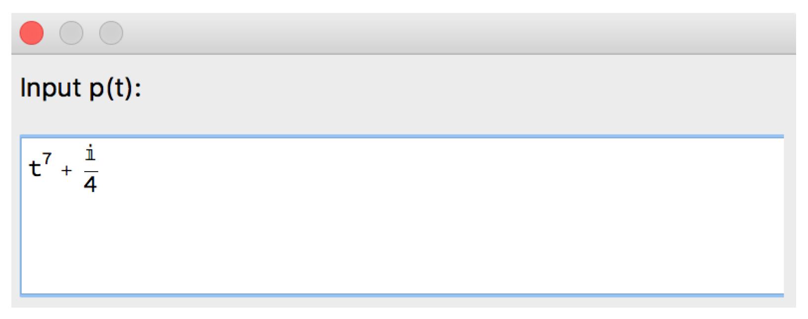
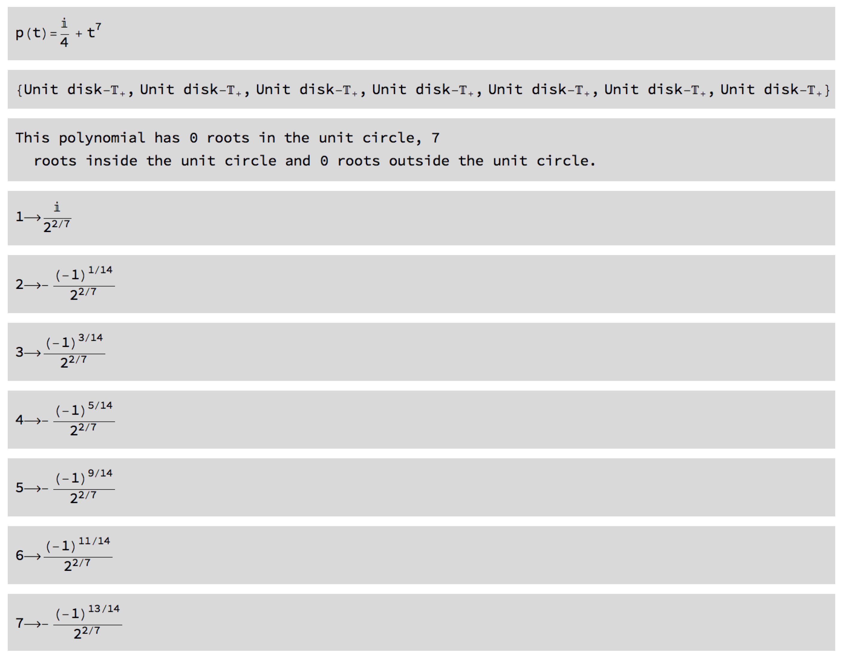
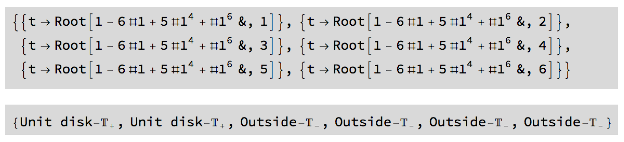
Example 10.

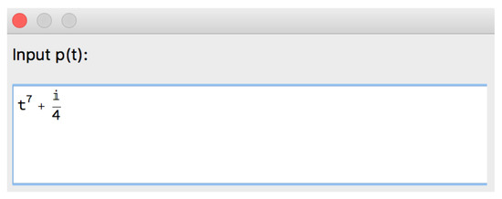
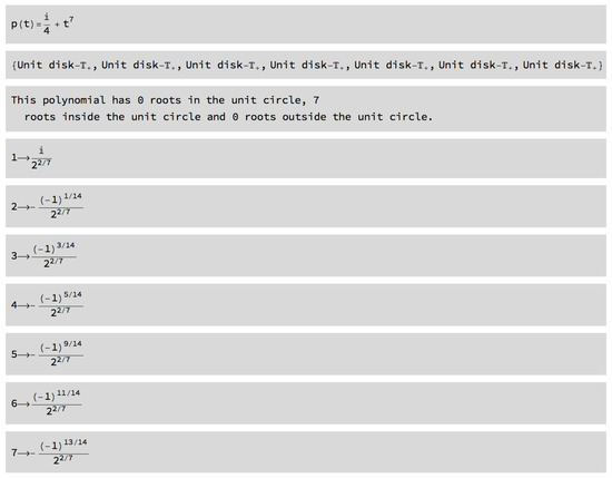
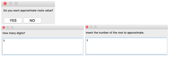
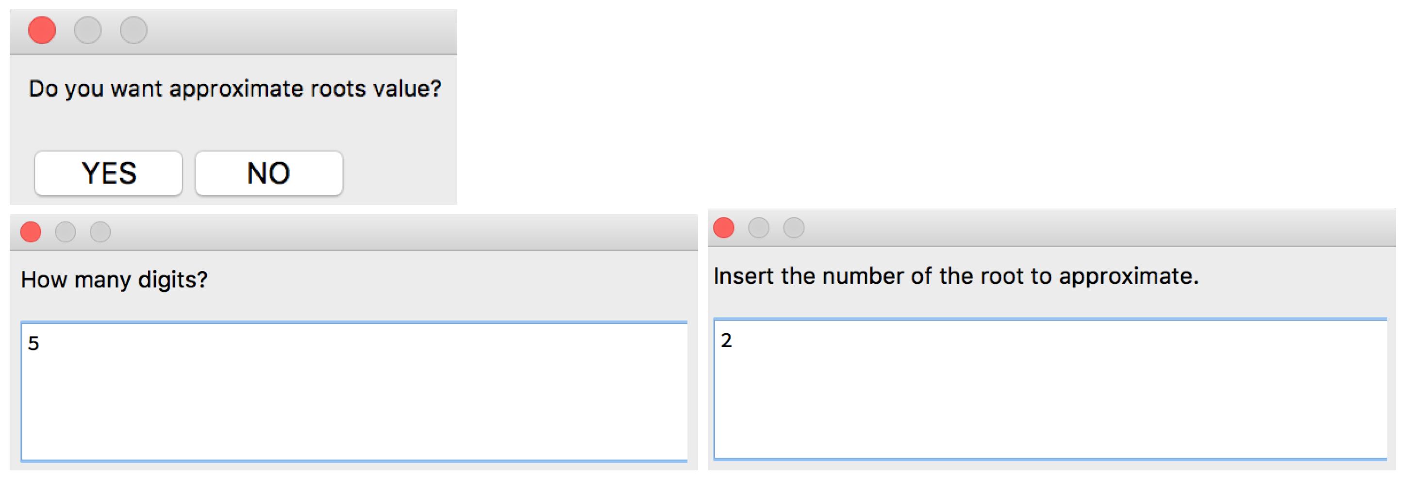
Let us insert directly the polynomial p (Figure 32). The algorithm gives the roots in $\mathbb{T}$, ${\mathbb{T}}_{+}$, and ${\mathbb{T}}_{-}$ (Figure 33) and gives the opportunity to the user to obtain an approximate value of the roots (Figure 34).

Figure 32. Part of the structure of the [ARoots] algorithm corresponding to the Option 1 to input p.

Figure 33. Output given by the [ARoots] algorithm.

Figure 34. Part of the structure of the [ARoots] algorithm corresponding to the option to get an approximate root value.

[ARoots] algorithm gives the extra output presented in Figure 35.

Figure 35. Output given by the [ARoots] algorithm.

Remark 5.

This example is related with Example 8 in Section 2.2.2.

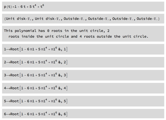
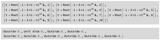
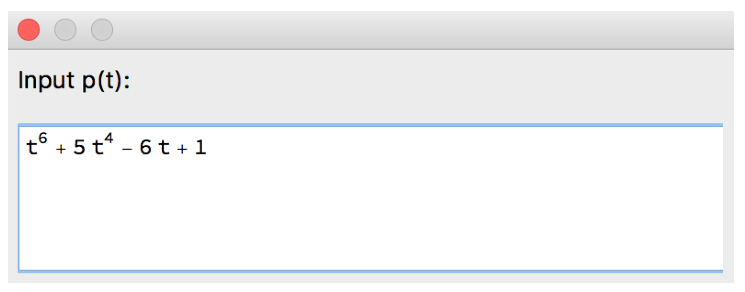
Example 11.

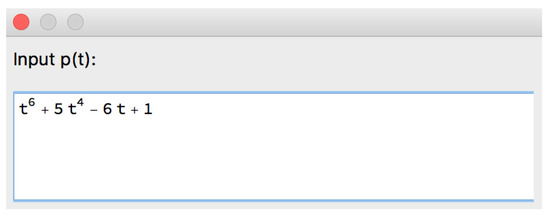
Let us insert directly the polynomial p (Figure 36).

Figure 36. Part of the structure of the [ARoots] algorithm corresponding to Option 1 to input p.

The algorithm gives the roots in $\mathbb{T}$, ${\mathbb{T}}_{+}$, and ${\mathbb{T}}_{-}$ (Figure 37).

Figure 37. Output given by the [ARoots] algorithm.

Even in this case, where the roots appear represented as Root objects (Mathematica uses Root objects to represent solutions of algebraic equations in one variable, when it is impossible to find explicit formulas for these solutions), it is possible to request approximate values. The Root object is not a mere denoting symbol but rather an expression that can be symbolically manipulated and numerically evaluated with any desired precision [1].

Remark 6.

This example is related with Example 9 in Section 2.2.2.

2.4. [AZeros] and [APoles] Algorithms

This subsection is dedicated to the formal description of the [AZeros] and [APoles] algorithms. These algorithms identify, given a list of complex numbers, their location relative to $\mathbb{T}$, ${\mathbb{T}}_{+}$, and ${\mathbb{T}}_{-}$.

The [AZeros] and [APoles] algorithms were created to be used as part of other more complex algorithms (as well as those described in Section 3), exploring a list of values entered by the user. In fact, the code of these algorithms was based on the code of the [ARoots] algorithm (Figure 38). However, these algorithms can also be used independently by using an nb format file where a rational function is introduced and Mathematica’s Solve command is used.

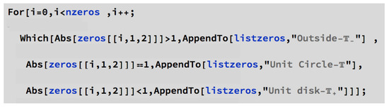
Figure 38. Part of the code structure of the [AZeros] algorithm code responsible for the location, relative to the unit circle, of complex numbers in a given list.

Figure 39 contains the flowcharts of the [AZeros] and [APoles] algorithms.

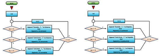
Figure 39. Flowcharts of the [AZeros] and [APoles] algorithms.

[AZeros] and [APoles] Algorithms Examples

Let us now present nontrivial examples computed with the algorithms. For an inputed rational function r defined in $\mathbb{T}$, the algorithm creates a list of complex numbers and gives the information of which zeros/poles are located in $\mathbb{T}$, ${\mathbb{T}}_{+}$, and ${\mathbb{T}}_{-}$.

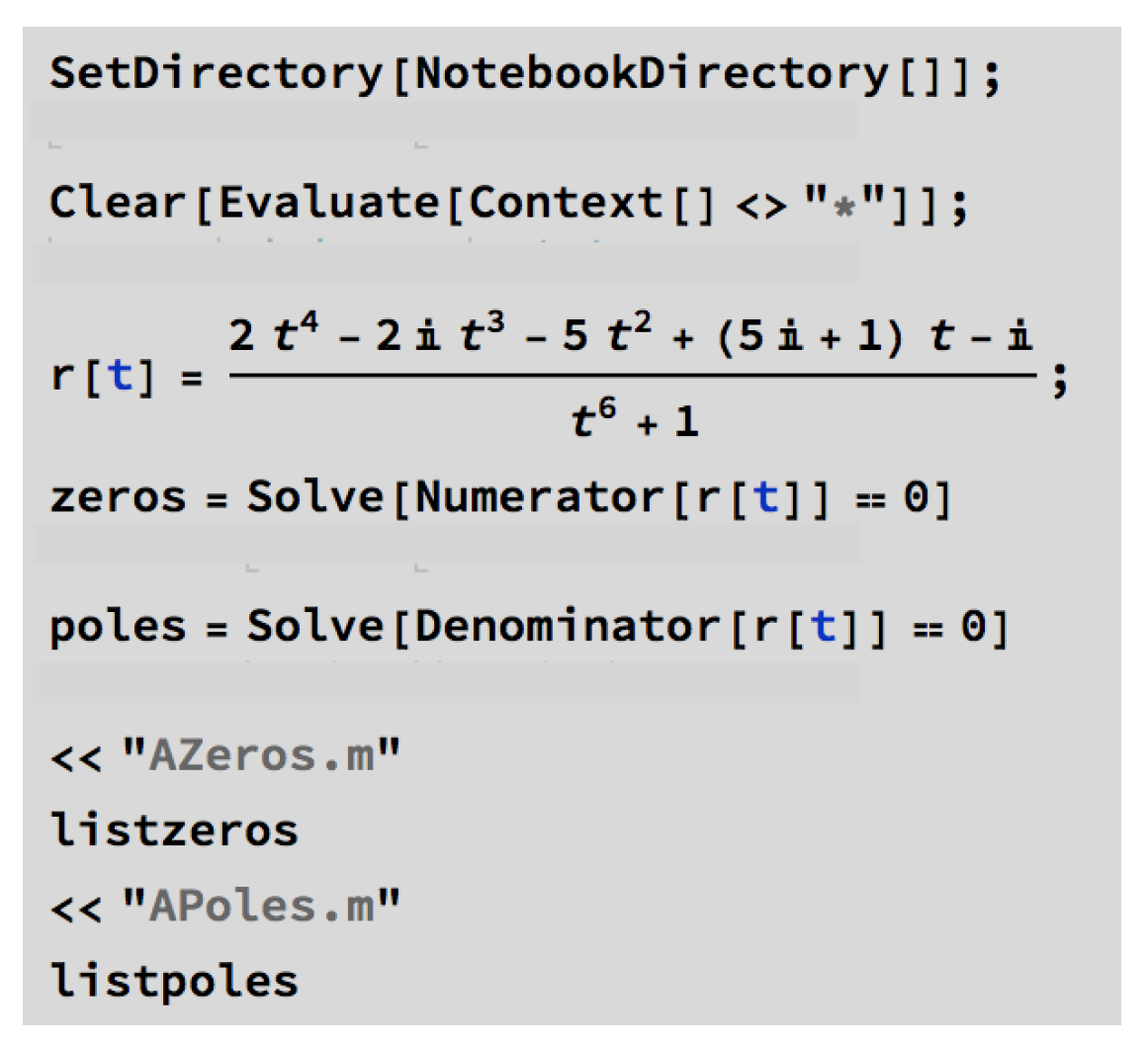
Example 12.

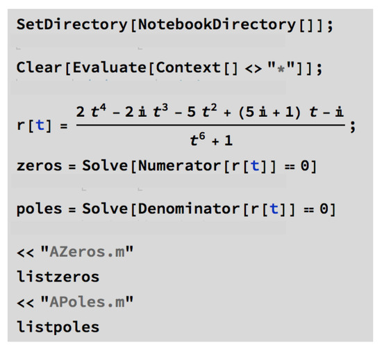
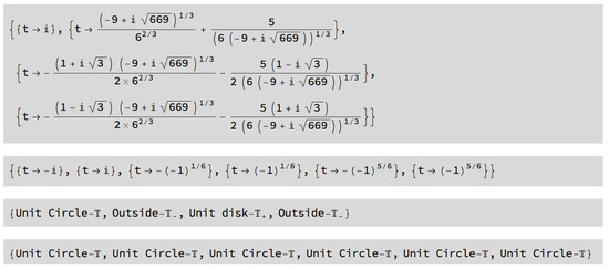
Let us use the nb format file associated with the [AZeros] and [APoles] algorithms that allows the input of a rational function r to compute its zeros and poles and locate them (Figure 40).

Figure 40. Part of the structure that allows the computation of the zeros and poles of r.

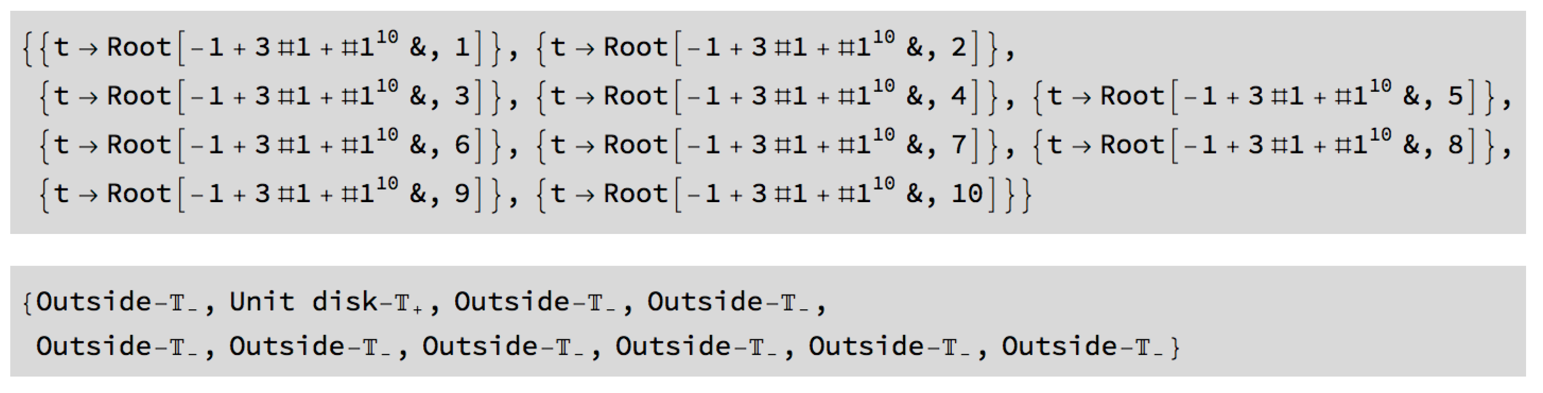
We obtain the output presented in Figure 41.

Figure 41. Output given by the [AZeros] and [APoles] algorithms.

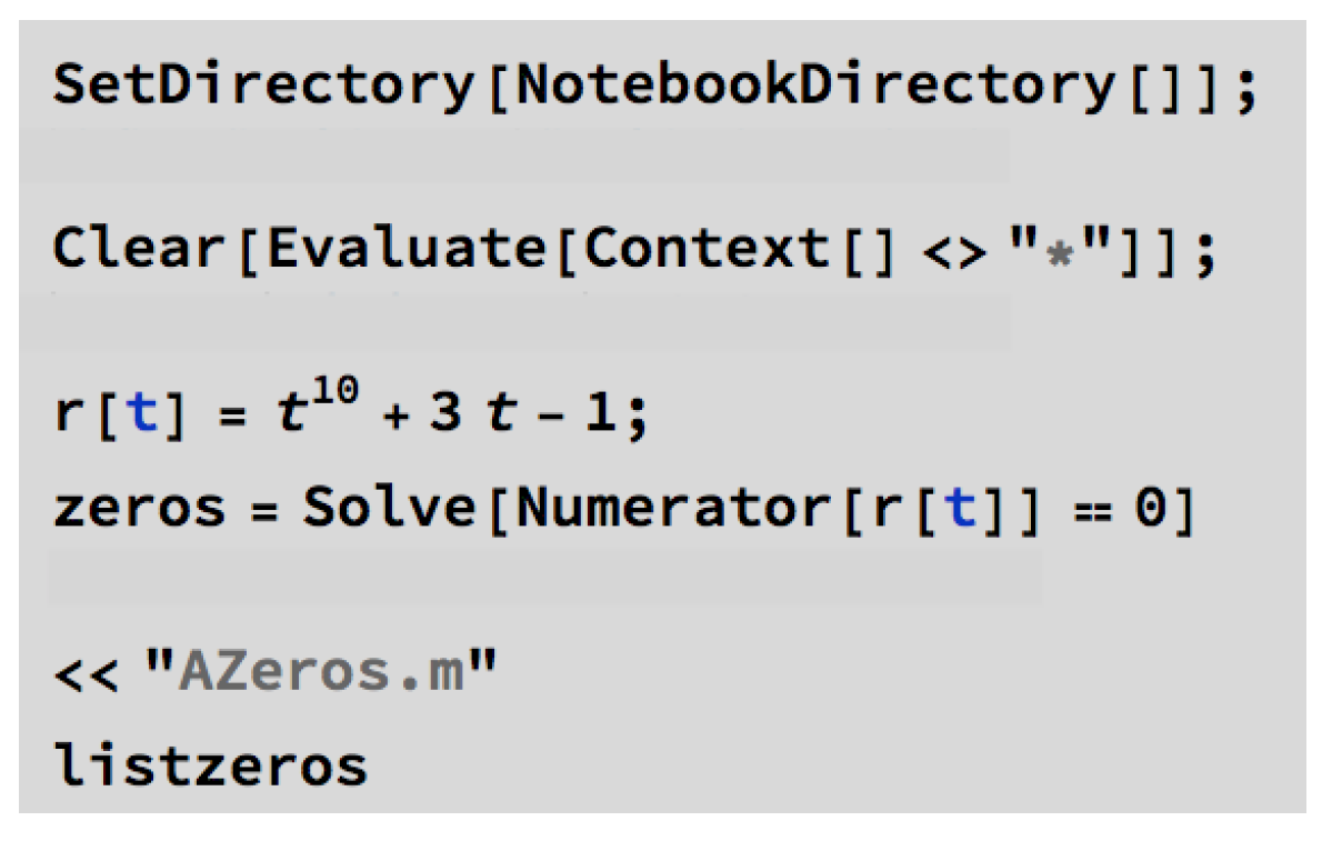
Example 13.

Let us use the nb format file associated with the [AZeros] algorithm that allows the input of a rational function r to compute its zeros and locate them (Figure 42).

Figure 42. Part of the structure that allows us to compute and locate zeros of r.

We obtain the output presented in Figure 43.

Figure 43. Output given by the [AZeros] algorithm.

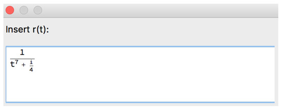
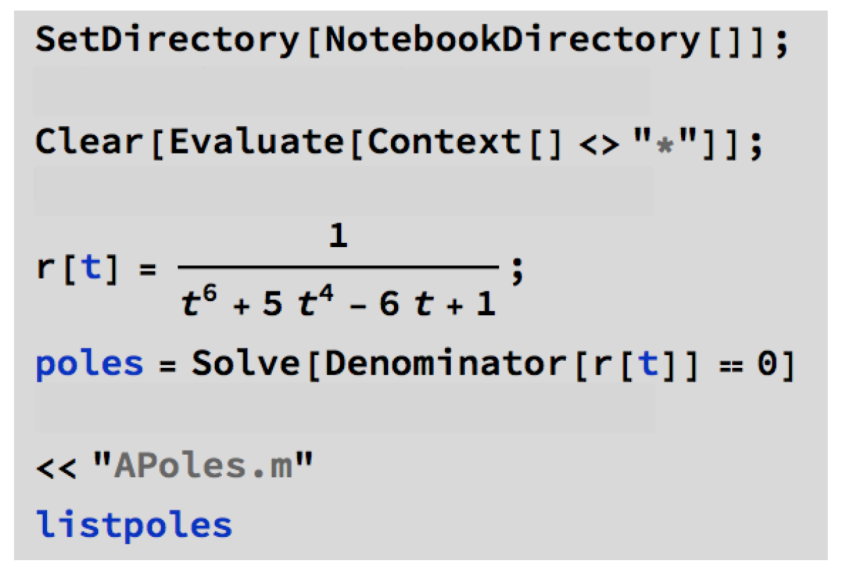
Example 14.

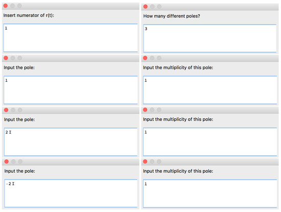
Let us use the nb format file associated with the [APoles] algorithm that allows the input of a rational function r to compute its poles and locate them (Figure 44).

Figure 44. Part of the structure that allows us to compute and locate poles of r.

We obtain the output presented in Figure 45, which is used in Example 21 in Section 3.

Figure 45. Output given by the [APoles] algorithm.

3. Results

This section is dedicated to the description of new operator theory algorithms. Some of them use the [AZeros] and [APoles] algorithms described in the previous section. Several nontrivial examples are presented. Section 3.1 is dedicated to the [ASPPlusPMinus] algorithm, which computes the singular integrals $S_{\mathbb{T}}r\left(t\right)$, $P_{+}r\left(t\right)$ and $P_{-}r\left(t\right)$ for a given rational function r. An improved version of the [SInt] algorithm is described in Section 3.2.

3.1. [ASPPlusPMinus] Algorithm

This subsection is dedicated to the formal description of the [ASPPlusPMinus] algorithm, which computes the singular integrals $S_{\mathbb{T}}r\left(t\right)$, $P_{+}r\left(t\right)$ and $P_{-}r\left(t\right)$ for a given rational function r. This algorithm validates the inputed rational function r, analyzing the location of its poles using the Root object concept. Thus, some of the incorrect outputs described in Section 2.2, and not considered in the implementation of the [SInt] algorithm [2], do not happen.

The design and implementation of this algorithm allowed the improvement of the [SInt] algorithm, creating the [SInt]${}_{2.0}$ algorithm described in Section 3.2.

Figure 46 contains the flowchart of the [ASPPlusPMinus] algorithm.

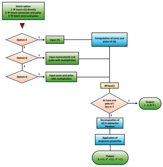
Figure 46. Flowchart of the [ASPPlusPMinus] algorithm.

The algorithm allows three input options for the rational function $r\left(t\right)$ (Figure 47).

Figure 47. Box with three options to insert the rational function r.

This algorithm integrates the [APoles] algorithm and uses parts of the [ARoots] algorithm, namely in the code structure where the Solve command is used (Figure 48). Several properties of the projection operators (2) are implemented so that the output is the singular integrals obtained by applying these operators to the rational function r and the singular integral (1).

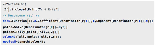
Figure 48. Part of the code structure of the [ASPPlusPMinus] algorithm that integrates the [APoles] algorithm and uses Mathematica’s Solve command.

[ASPPlusPMinus] Algorithm Examples

Let us now present nontrivial examples computed with the [ASPPlusPMinus] algorithm. For each inputed rational function r, defined in $\mathbb{T}$, the algorithm validates whether the function belongs to algebra $\mathcal{R}\left(\mathbb{T}\right)$ and, if so, computes the singular integrals $S_{\mathbb{T}}r\left(t\right)$, $P_{+}r\left(t\right)$, and $P_{-}r\left(t\right)$.

Example 15.

Let us use Option 2 to input the rational function r (Figure 49).

Figure 49. Part of the structure of the [ASPPlusPMinus] algorithm corresponding to Option 2 to input r.

[ASPPlusPMinus] algorithm gives the output presented in Figure 50.

Figure 50. Output given by the [ASPPlusPMinus] algorithm.

Remark 7.

This example considers the same rational function r as Example 4 but gives a correct output.

Example 16.

Let us use Option 1 to input the rational function r (Figure 51).

Figure 51. Part of the structure of the [ASPPlusPMinus] algorithm corresponding to Option 1 to input r.

[ASPPlusPMinus] algorithm gives the output presented in Figure 52.

Figure 52. Output given by the [ASPPlusPMinus] algorithm.

Remark 8.

This example considers the same rational function as Example 8 but gives a correct output.

Example 17.

Let us use Option 1 to input the rational function r (Figure 53).

Figure 53. Part of the structure of the [ASPPlusPMinus] algorithm corresponding to Option 1 to input r.

The [ASPPlusPMinus] algorithm, usingRootobjects, gives the output presented in Figure 54.

Figure 54. Output given by the [ASPPlusPMinus] algorithm.

Remark 9.

This example considers the same rational function r as Example 9 but gives a correct output.

3.2. [SInt]${}_{2.0}$ Algorithm

This subsection is dedicated to a formal description of the [SInt]${}_{2.0}$ algorithm (An improved version of the [SInt] algorithm described in [2].), which computes the singular integrals $S_{\mathbb{T}}X\left(t\right)$ and $S_{\mathbb{T}}Y\left(t\right)$ for given functions $X\left(t\right)=r\left(t\right)x_{+}\left(t\right)$ and $Y\left(t\right)=r\left(t\right)y_{-}\left(t\right)$, where $x_{+},\overline{y_{-}}\in H_{\infty }\left(\mathbb{T}\right)$ and $r\in \mathcal{R}\left(\mathbb{T}\right)$.

This algorithm validates the inputed rational function r, analyzing the location of its poles using the Root object concept and Mathematica’s Solve command. In the case when particular rational functions $x_{+}$ and $y_{-}$ are inputed, the algorithm also checks if $x_{+}$ and $\overline{y_{-}}$ have poles at $\mathbb{T}\cup {\mathbb{T}}_{+}$. Thus, the incorrect outputs described in Section 2.2, and not considered in the implementation of the [SInt] algorithm [2], do not happen. However, it cannot validate functions $x_{+}$ and $y_{-}$, which are not rational functions (Example 22). In this case, the algorithm provides the general expression of the singular integrals $S_{\mathbb{T}}X\left(t\right)$ and $S_{\mathbb{T}}Y\left(t\right)$ in terms of projection operator $P_{+}$ but does not give an incorrect output (as the [SInt] algorithm).

The flowchart of the [SInt]${}_{2.0}$ algorithm is presented in Figure 55.

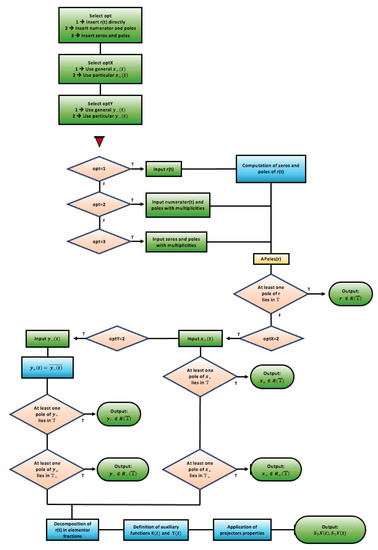
Figure 55. Flowchart of the [SInt]${}_{2.0}$ algorithm.

This algorithm integrates parts of the code structure of the [ASPPlusPMinus] algorithm and uses similar methodologies to validate inputed functions $x_{+}$ and $y_{-}$ in the rational case (Figure 56).

Figure 56. Part of the code structure of the [SInt]${}_{2.0}$ algorithm responsible for validating $x_{+}$.

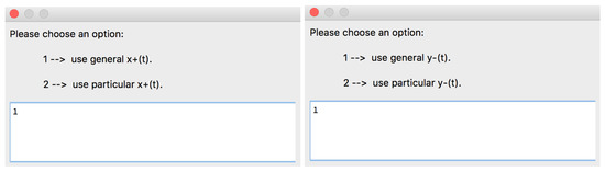
There are three options to insert the rational function $r\left(t\right)$. Functions $x_{+}$ and $y_{-}$ can be particular functions or functions in their general form (Figure 57).

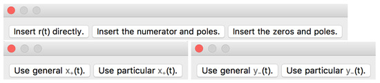
Figure 57. Part of the code structure of the [SInt]${}_{2.0}$ algorithm responsible for the input options.

If $x_{+}$ is a rational function introduced in a particular way, the algorithm checks if $x_{+}$ has poles in the unit circle or in ${\mathbb{T}}_{+}$, and similarly, the algorithm checks if the rational function $\overline{y_{-}}$ has poles in $\mathbb{T}\cup {\mathbb{T}}_{+}$.

In order to facilitate the algorithm user’s task, this new algorithm was designed to allow the entire program to run and all options to be requested through boxes.

It should be noted that in this new version, considering that it analyzes the validity of functions $x_{+}$ and $y_{-}$ when introduced as particular rational functions, the use of arbitrary constants is not allowed (as in Example 1).

[SInt]${}_{2.0}$ Algorithm Examples

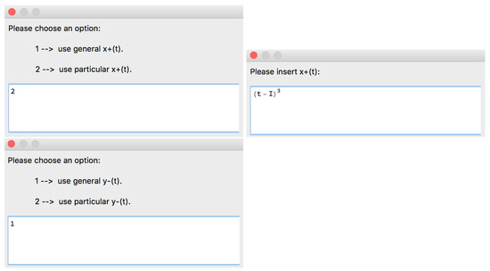
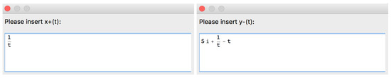
Example 18.

Let us use Option 1 to input the rational function r and consider particular functions $x_{+}$ and $y_{-}$ (Figure 58).

Figure 58. Part of the structure of the [SInt]${}_{2.0}$ algorithm responsible for the input options.

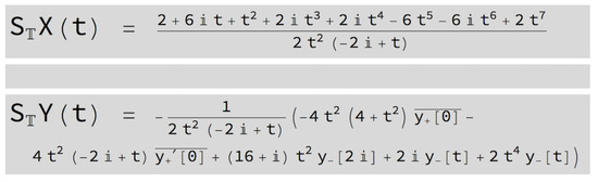
In this example, as the function $x_{+}$ is not validated by the algorithm ($x_{+}\notin \mathcal{R}\left(\mathbb{T}\right)$), it is not possible to input any particular function $y_{-}$. The output presented in Figure 59 is obtained.

Figure 59. Output given by the [SInt]${}_{2.0}$ algorithm.

Remark 10.

This example considers the same function $x_{+}$ as Example 5 but gives a correct output.

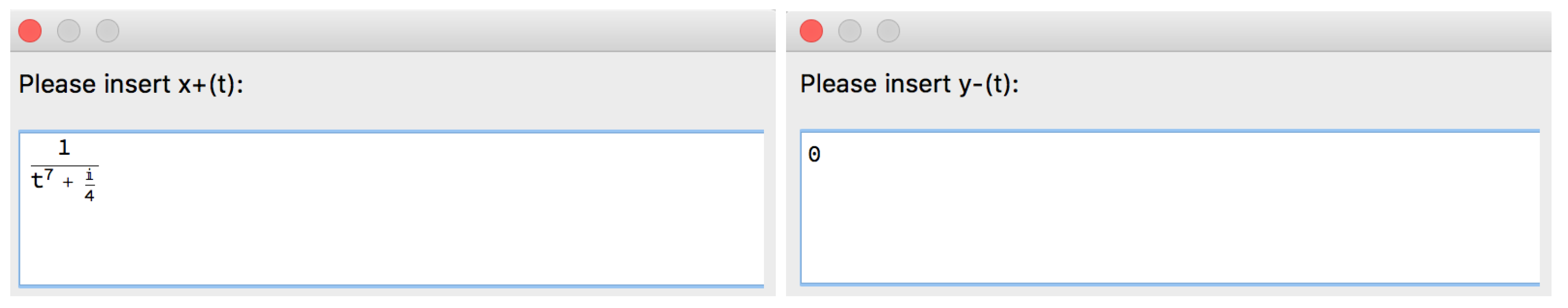
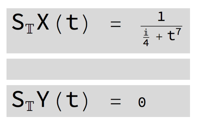
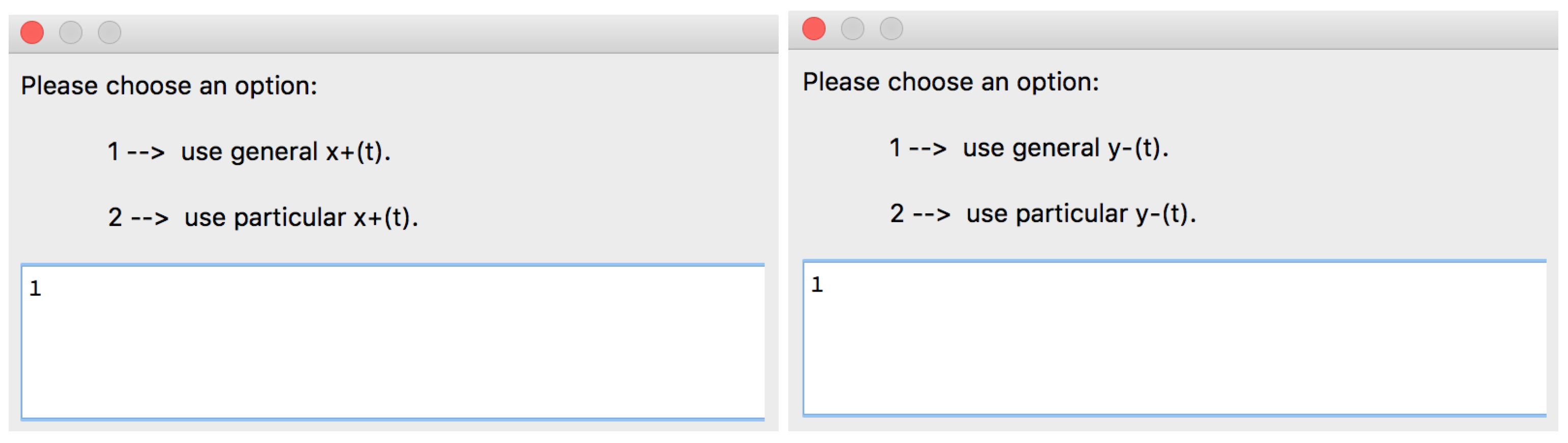
Example 19.

Let us use Option 1 to input the rational function r and consider particular functions $x_{+}$ and $y_{-}$ (Figure 60).

Figure 60. Part of the structure of the [SInt]${}_{2.0}$ algorithm responsible for the input options.

In this example, as the function $x_{+}$ is not validated by the algorithm ($x_{+}\notin {\mathcal{R}}_{+}\left(\mathbb{T}\right)$), it is not possible to input any particular function $y_{-}$. The output presented in Figure 61 is obtained.

Figure 61. Output given by the [SInt]${}_{2.0}$ algorithm.

Remark 11.

This example considers the same function $x_{+}$ as Example 6 but gives a correct output.

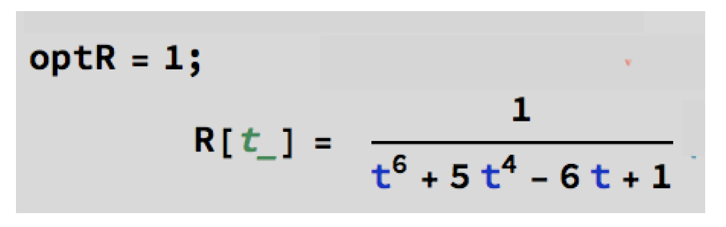
Example 20.

Let us use Option 1 to input the rational function r and a particular function $x_{+}$ (Figure 62). Let us consider a general expression for the function $y_{-}$.

Figure 62. Part of the structure of the [SInt]${}_{2.0}$ algorithm responsible for the input options.

In this example, despite the polynomial degree of the denominator of the function $x_{+}$, it is possible to identify that $x_{+}$ is not a valid function.

The output presented in Figure 63 is obtained.

Figure 63. Output given by the [SInt]${}_{2.0}$ algorithm.

Remark 12.

This example considers the same function $x_{+}$ as Example 8 but gives a correct output.

Example 21.

Let us use Option 1 to input the rational function r (Figure 64). Let us consider general expressions for the functions $x_{+}$ and $y_{-}$.

Figure 64. Part of the structure of the [SInt]${}_{2.0}$ algorithm responsible for the input options.

In this example, despite the polynomial degree of the denominator of the function r, it is possible to compute the singular integrals.

The output presented in Figure 65 is obtained.

Figure 65. Output given by the [SInt]${}_{2.0}$ algorithm.

Remark 13.

This example considers the same function r as Example 9 but gives a correct output in terms of Root objects.

Example 22.

Let us use Option 1 to input the rational function r and consider particular functions $x_{+}$ and $y_{-}$ (Figure 66).

Figure 66. Part of the structure of the [SInt]${}_{2.0}$ algorithm responsible for the input options.

In this example, as $x_{+}$ is not a rational function, the algorithm cannot identify that it is a valid function. The [SInt]${}_{2.0}$ algorithm provides the general expression of the singular integrals $S_{\mathbb{T}}X\left(t\right)$ and $S_{\mathbb{T}}Y\left(t\right)$ in terms of projection operator $P_{+}$, but does not give an incorrect output (as in the [SInt] algorithm).

Remark 14.

In order to improve the version described in [2], it was necessary to eliminate some of the properties included in the [SInt] code (Figure 67).

Figure 67. Piece of code removed from [SInt] algorithm.

We obtain the output presented in Figure 68.

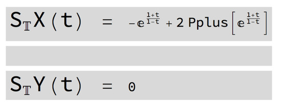
Figure 68. Output given by the [SInt]${}_{2.0}$ algorithm.

4. Discussion

The design of our analytical algorithms is focused on the possibility of implementing on a computer all, or a significant part, of the extensive symbolic and numeric calculations present in the algorithms. The methods developed rely on innovative techniques of operator theory and have a great potential for extension to more complex and general problems.

• We hope that our work within operator theory, and with Mathematica, will help in the path to the future design and implementation of several other analytical algorithms, with numerous applications in many areas of research and technology;
• We are considering the design and implementation of other factorization, spectral and kernel algorithms;
• It is our opinion that the design and implementation of analytical algorithms that work with singular integral operators defined on the real line can constitute a very interesting new line of research;
• We also hope that, going forward, these analytical methods, and their implementation using a computer algebra system with large symbolic and numeric computation capabilities, may contribute to the numerical approach in operator theory.

References

- Conceição, A.C. Symbolic Computation Applied to the Study of the Kernel of Special Classes of Paired Singular Integral Operators. Math. Comput. Sci. 2021, 15, 63–90. [Google Scholar] [CrossRef]
- Conceição, A.C.; Kravchenko, V.G.; Pereira, J.C. Computing some classes of Cauchy type singular integrals with Mathematica software. Adv. Comput. Math. 2013, 39, 273–288. [Google Scholar] [CrossRef]
- Conceição, A.C.; Kravchenko, V.G.; Pereira, J.C. Rational functions factorization algorithm: A symbolic computation for the scalar and matrix cases. In Proceedings of the 1st National Conference on Symbolic Computation in Education and Research, Lisboa, Portugal, 2–3 April 2012. [Google Scholar]
- Conceição, A.C.; Kravchenko, V.G.; Pereira, J.C. Factorization Algorithm for Some Special Non-rational Matrix Functions. In Operator Theory: Advances and Applications; Birkhäuser Verlag: Basel, Switzerland, 2010; Volume 202, pp. 87–109. [Google Scholar]
- Conceição, A.C.; Pereira, J.C. Exploring the spectra of some classes of singular integral operators with symbolic computation. Math. Comput. Sci. 2016, 10, 291–309. [Google Scholar] [CrossRef]
- Conceição, A.C.; Kravchenko, V.G. About explicit factorization of some classes of non-rational matrix functions. Math. Nachr. 2007, 280, 1022–1034. [Google Scholar] [CrossRef]
- Castro, L.P.; Rojas, E.M.; Saitoh, S.; Tuan, N.M. Solvability of singular integral equations with rotations and degenerate kernels in the vanishing coefficient case. Anal. Appl. 2015, 13, 1–21. [Google Scholar] [CrossRef] [Green Version]
- Conceição, A.C.; Marreiros, R.C.; Pereira, J.C. Symbolic computation applied to the study of the kernel of a singular integral operator with non-Carleman shift and conjugation. Math. Comput. Sci. 2016, 10, 365–386. [Google Scholar] [CrossRef]
- Ablowitz, M.J.; Clarkson, P.A. Solitons, Nonlinear Evolution Equations and Inverse Scattering; Cambridge University Press: Cambridge, UK, 1991. [Google Scholar]
- Aktosun, T.; Klaus, M.; van der Mee, C. Explicit Wiener–Hopf factorization for certain non-rational matrix functions. Integral Equ. Oper. Theory 1992, 15, 879–900. [Google Scholar] [CrossRef]
- Clancey, K.; Gohberg, I. Factorization of Matrix Functions and Singular Integral Operators. In Operator Theory: Advances and Applications; Birkhäuser Verlag: Basel, Switzerland, 1981. [Google Scholar]
- Faddeev, L.D.; Takhatayan, L. Hamiltonian Methods in the Theory of Solitons; Springer: Berlin, Germany, 1987. [Google Scholar]
- Kravchenko, V.G.; Litvinchuk, G.S. Introdution to the Theory of Singular Integral Operators with Shift; Kluwer Academic Publishers: Dordrecht, The Netherlands, 1994. [Google Scholar]
- Litvinchuk, G.S. Solvability Theory of Boundary Value Problems and Singular Integral Equations with Shift; Kluwer Academic Publishers: Dordrecht, The Netherlands, 2000. [Google Scholar]
- Litvinchuk, G.S.; Spitkovskii, I.M. Factorization of Measurable Matrix Functions. In Operator Theory: Advances and Applications; Birkhäuser: Basel, Switzerland, 1987. [Google Scholar]
- Prössdorf, S. Some Classes of Singular Equations; Elsevier: Amsterdam, The Netherlands, 1978. [Google Scholar]
- Gohberg, I.; Krupnik, N. One-Dimensional Linear Singular Integral Equations. In Operator Theory: Advances and Applications; Birkhäuser: Basel, Switzerland, 1992. [Google Scholar]
Publisher’s Note: MDPI stays neutral with regard to jurisdictional claims in published maps and institutional affiliations. |
© 2021 by the authors. Licensee MDPI, Basel, Switzerland. This article is an open access article distributed under the terms and conditions of the Creative Commons Attribution (CC BY) license (https://creativecommons.org/licenses/by/4.0/).