A Hybrid Function Approach to Solving a Class of Fredholm and Volterra Integro-Differential Equations

Abstract

In this paper, we use a numerical method that involves hybrid and block-pulse functions to approximate solutions of systems of a class of Fredholm and Volterra integro-differential equations. The key point is to derive a new approximation for the derivatives of the solutions and then reduce the integro-differential equation to a system of algebraic equations that can be solved using classical methods. Some numerical examples are dedicated for showing the efficiency and validity of the method that we introduce.

1. Introduction

It is well-known that integral equations reign over many mathematical models of various phenomena in mathematics, physics, economy, biology, engineering and other fields. Several explanatory examples of such models can be found in the literature and several mathematical physics, applied mathematics, and engineering problems are reduced to Volterra–Fredholm integral equations. More precisely, scientific researchers have explored the topic of integro-differential equations through their work in various fields of science such as physics [1], biology [2] and engineering [3,4] and in numerous applications such as heat transfer, neurosciences [5], diffusion process, neutron diffusion, biological species [6,7], biomechanics, economics, electrical engineering, electrodynamics, electrostatics, filtration theory, fluid dynamics, game theory, oscillation theory, queuing theory [8], airfoil theory [9], elastic contact problems [10,11], fracture mechanics [12], combined infrared radiation, molecular conduction [13] and so on.

In recent years, many different basic functions have been used to estimate the solution of integral equations, such as orthogonal functions and wavelets. Three families of the orthogonal functions are classified: piecewise constant orthogonal functions (e.g., Walsh, Haar, block-pulse, etc.), orthogonal polynomials (e.g., Legendre, Laguerre, Chebyshev, etc.) and sine–cosine functions in the Fourier series. For instance, many authors investigated the general k-th order integro-differential equation

$$\begin{array}{c}\hfill y^{\left(k\right)}\left(t\right)+l\left(t\right)y\left(t\right)+{\int }_a^{b}g(t,s)y^{\left(m\right)}\left(s\right)ds=f\left(t\right),\end{array}$$

(1)

with initial conditions

$$y\left(a\right)=a_0,\cdots ,y^{(n-1)}\left(a\right)=a_{n-1},$$

where $a_0,\dots ,a_{n-1}$ are real constants, $k,m$ are positive integers and $m<k$, the functions $l,f,g$ are given and $y\left(t\right)$ is the solution to be determined. In [14], the authors applied the homotopy perturbation method to solve Equation (1), while in [15,16], the authors changed the equation to an ordinary integro-differential equation and applied the variational iteration method to solve it so that the Lagrange multipliers can be effectively identified. Using the operational matrix of derivatives of hybrid functions, a numerical method has been presented in [17] to solve Equation (1). In [18], Hemeda used the iterative method introduced in [19] to solve the more general equation

$$\begin{array}{c}\hfill y^{\left(k\right)}\left(t\right)+l\left(t\right)y\left(t\right)+{\int }_a^{b}g(t,s)y^{\left(n\right)}\left(s\right)y^{\left(m\right)}\left(s\right)ds=f\left(t\right),\end{array}$$

(2)

where $n\le m<q$.

In this paper, we use block-pulse and hybrid functions to approximate solutions $y\left(t\right)$ of the Fredholm integro-differential system given by

$$\begin{array}{c}\hfill \left\{\begin{array}{c}y\left(t\right)+\lambda {\int }_0^{1}k(t,s)y^{\left(m\right)}\left(s\right)y^{\left(n\right)}\left(s\right)ds=f\left(t\right),\hfill \\ y\left(0\right)=a_0,\cdots ,y^{\left(l\right)}\left(0\right)=a_l,\hfill \end{array}\right.\end{array}$$

(3)

and solutions $y\left(t\right)$ of the Volterra integro-differential system given by

$$\begin{array}{c}\hfill \left\{\begin{array}{c}y\left(t\right)+\beta {\int }_0^{t}g(t,s)y^{\left(m\right)}\left(s\right)y^{\left(n\right)}\left(s\right)ds=f\left(t\right),\hfill \\ y\left(0\right)=a_0,\cdots ,y^{\left(l\right)}\left(0\right)=a_l.\hfill \end{array}\right.\end{array}$$

(4)

Here $m,n$ are positive integers, $l=\max (m,n)-1$, $a_0,\cdots ,a_l$ are initial conditions, the parameters $\beta ,\lambda$ and the functions $k(t,s),g(t,s)$ and $f\left(t\right)$ are known and belong to $L^2[0,1)$. The function $y\left(t\right)$, as well as its derivatives $y^{\left(n\right)}$ and $y^{\left(m\right)}$, are unknown. We point out that System (3) is a particular case of Equation (2).

Hybrid functions have been applied extensively for solving differential systems and proved to be a useful mathematical tool. The pioneering work via hybrid functions was led by the authors in [20,21], who first derived an operational matrix for the integral of the hybrid function vector, and paved the way for the hybrid function analysis of the dynamic systems. Since then, the hybrid functions’ approach has been improved and used to approximate differential equations or systems (see [22,23,24,25,26,27,28] and the references therein).

The novelty and the key point in solving Systems (3) and (4) are to use some useful properties of hybrid functions to derive a new approximation $Y^{\left(n\right)}$ of the derivative $y^{\left(n\right)}\left(t\right)$ of order n of the solution $y\left(t\right)$ (see Lemma 1). Hence, Systems (3) and (4) can be converted into reduced algebraic systems.

For arbitrary positive integers q and r, the set $\left\{b_{km}\left(t\right)\right\},k=1,2,\cdots ,q,m=0,1,\cdots ,r-1$ of hybrid functions will be used to approximate the solution $y_{r-1}\left(t\right)$ of the given system of integro-differential equations. This approximate solution will involve Legnedre polynomials of degree $r-1$ defined on q subintervals of $[0,1]$.

This paper is organized as follows: in Section 2, we introduce hybrid functions and its properties. In Section 3, we describe the method for approximating solutions of the Fredholm and Volterra integro-differential Systems (3) and (4). An upper bound of the error is given in Section 4, and finally numerical results are reported in Section 5.

2. Preliminaries

In this section, we define the Legendre polynomials $p_m\left(t\right)$, as well as block-pulse and hybrid functions. We also recall functions’ approximation in the Hilbert space $L^2[-1,1]$.

The Legendre polynomials $p_m\left(t\right)$ are polynomials of degree m defined on the interval $[-1,1]$ by

$$p_m\left(t\right)=\sum _{k=0}^M\frac{{(-1)}^k(2m-2k)!}{2^{m}k!(m-k)!(m-2k)!}{t}^{m-2k},m\in \mathbb{N},$$

where $M=\left\{\begin{array}{c}\frac{m}{2},\mathrm{if}m\mathrm{is}\mathrm{even},\hfill \\ \frac{m-1}{2},\mathrm{if}m\mathrm{is}\mathrm{odd}.\hfill \end{array}\right.$

Equivalently, the Legendre polynomials are given by the recursive formula (see [6,23,29,30])

$$\begin{array}{c}{p}_0\left(t\right)=1,p_1\left(t\right)=t,\hfill \\ p_{m+1}\left(t\right)=\frac{2m+1}{m+1}t{p}_m\left(t\right)-\frac{m}{m+1}{p}_{m-1}\left(t\right),m=1,2,3,\cdots .\hfill \end{array}$$

The set $\{p_m\left(t\right);t=0,1,\cdots \}$ is a complete orthogonal system in $L^2[-1,1]$.

Definition 1.

[6,23,29] For an arbitrary positive integer q, let ${\left\{b_k\left(t\right)\right\}}_{k=1}^q$ be the finite set of block-pulse functions on the interval $[0,1)$ defined by

$$\begin{array}{c}\hfill b_k\left(t\right)=\left\{\begin{array}{c}1,if\frac{k-1}{q}\le t<\frac{k}{q},\hfill \\ 0,elsewhere.\hfill \end{array}\right.\end{array}$$

The block-pulse functions are disjoint and have the property of orthogonality on $[0,1)$, since for $i,j=1,2,\cdots ,q$, we have:

$$\begin{array}{c}\hfill b_i\left(t\right)b_j\left(t\right)=\left\{\begin{array}{c}0,\mathrm{if}i\ne j,\hfill \\ b_i\left(t\right),\mathrm{if}i=j,\hfill \end{array}\right.\end{array}$$

and

$$\begin{array}{c}\hfill ⟨b_i\left(t\right),b_j\left(t\right)⟩=\left\{\begin{array}{c}0,\mathrm{if}i\ne j,\hfill \\ \frac{1}{q},\mathrm{if}i=j,\hfill \end{array}\right.\end{array}$$

where $⟨.,.⟩$ is the scalar product given by $⟨f,g⟩={\int }_0^{1}f\left(t\right)g\left(t\right)dt$, for any functions $f,g\in L^2[0,1)$.

Definition 2.

[6,23,29,30] Let r be an arbitrary positive integer. The set of hybrid functions $\left\{b_{km}\left(t\right)\right\},k=1,2,\cdots ,q,m=0,1,\cdots ,r-1$, where k is the order for block-pulse functions, m is the order for Legendre polynomials and t is the normalized time, is defined on the interval $[0,1)$ as

$$\begin{array}{c}\hfill b_{km}\left(t\right)=\left\{\begin{array}{c}{p}_m(2qt-2k+1),if\frac{k-1}{q}\le t<\frac{k}{q},\hfill \\ 0,elsewhere.\hfill \end{array}\right.\end{array}$$

Since $b_{km}\left(t\right)$ is the combination of Legendre polynomials and block-pulse functions which are both complete and orthogonal, then the set of hybrid functions is a complete orthogonal system in $L^2[0,1)$.

We are now able to define the vector function $B\left(t\right)$ of hybrid functions on $[0,1)$ by

$$B\left(t\right)={\left(B_1^T\left(t\right),\cdots ,B_q^T\left(t\right)\right)}^T,$$

where $B_i\left(t\right)={\left(b_{i0}\left(t\right),\cdots ,b_{i(r-1)}\left(t\right)\right)}^T$, for $i=1,2,\cdots ,q$, and $V^T$ denotes the transpose of a vector V.

Function approximation [6,23,29,30]: every function $f\left(t\right)\in L^2[0,1)$ can be approximated as

$$f\left(t\right)\simeq \sum _{k=1}^q\sum _{m=0}^{r-1}{f}_{km}{b}_{km}\left(t\right),$$

where

$$f_{km}=\frac{⟨f\left(t\right),b_{km}\left(t\right)⟩}{⟨b_{km}\left(t\right),b_{km}\left(t\right)⟩},\forall k=1,\cdots ,q,\forall m=0,\cdots ,r-1.$$

Thus,

$$\begin{array}{c}\hfill f\left(t\right)\simeq F^{T}B\left(t\right)=B^T\left(t\right)F,\end{array}$$

(5)

where F is the $rq\times 1$ column vector having $f_{km}$ as entries. In a similar way, any function $g(t,s)\in L^2\left([0,1)\times [0,1)\right)$ can be approximated as

$$\begin{array}{c}\hfill g(t,s)\simeq B^T\left(t\right)GB\left(s\right),\end{array}$$

(6)

where $G=\left(g_{ij}\right)$ is an $rq\times rq$ matrix given by

$$g_{ij}=\frac{⟨B_{\left(i\right)}\left(t\right),⟨g(t,s),B_{\left(j\right)}\left(s\right)⟩⟩}{⟨B_{\left(i\right)}\left(t\right),B_{\left(i\right)}\left(t\right)⟩⟨B_{\left(j\right)}\left(s\right),B_{\left(j\right)}\left(s\right)⟩},i,j=1,2,\cdots ,rq,$$

and $B_{\left(i\right)}\left(t\right)$ (resp. $B_{\left(j\right)}\left(s\right)$) denotes the $i^{th}$ component (resp. the $j^{th}$ component) of $B\left(t\right)$ (resp. $B\left(s\right)$).

Operational matrix of integration [6,23,29,30]: The integration of the vector function $B\left(t\right)$ may be approximated by ${\int }_0^{t}B\left(t^{\prime }\right)d{t}^{\prime }\simeq PB\left(t\right)$, where P is an $rq\times rq$ matrix known as the operational matrix of integration and given by

$$P=\left(\begin{array}{ccccc}E& H& H& ...& H\\ 0& E& H& ...& H\\ 0& 0& E& ...& ...\\ .& .& .& ...& H\\ 0& 0& 0& ...& E\end{array}\right)$$

where H and E are $r\times r$ matrices defined by

$$H=\frac{1}{q}\left(\begin{array}{ccccc}1& 0& 0& ...& 0\\ 0& 0& 0& ...& 0\\ 0& 0& 0& ...& 0\\ .& .& .& ...& 0\\ 0& 0& 0& ...& 0\end{array}\right)$$

and

$$E=\frac{1}{2q}\left(\begin{array}{cccccccc}1& 1& 0& 0& ...& 0& 0& 0\\ -\frac{1}{3}& 0& \frac{1}{3}& 0& ...& 0& 0& 0\\ 0& -\frac{1}{5}& 0& \frac{1}{5}& ...& 0& 0& 0\\ ..& ..& ..& ..& ...& ..& ..& ..\\ 0& 0& 0& 0& ...& -\frac{1}{2r-3}& 0& \frac{1}{2r-3}\\ 0& 0& 0& 0& ...& 0& -\frac{1}{2r-1}& 0\end{array}\right).$$

The integration of two hybrid functions [6,23,29,30]: the integration of the cross product of two hybrid function vectors is given by $L={\int }_0^{1}B\left(t\right)B^T\left(t\right)dt,$ where L is the $rq\times rq$ diagonal matrix defined by

$$L=\left(\begin{array}{cccccccc}D& 0& 0& 0& ...& 0& 0& 0\\ 0& D& 0& 0& ...& 0& 0& 0\\ ..& ..& ..& ..& ...& ..& ..& ..\\ ..& ..& ..& ..& ...& D& ..& ..\\ 0& 0& 0& 0& ...& 0& D& 0\\ 0& 0& 0& 0& ...& 0& 0& D\end{array}\right)$$

where D is the $r\times r$ matrix given by

$$D=\frac{1}{q}\left(\begin{array}{cccccccc}1& 0& 0& 0& ...& 0& 0& 0\\ 0& \frac{1}{3}& 0& 0& ...& 0& 0& 0\\ ..& ..& ..& ..& ...& ..& ..& ..\\ 0& 0& 0& 0& ...& 0& 0& \frac{1}{2r-1}\end{array}\right).$$

The matrix $\tilde{C}$ associated to a vector C [6,22,23,30]: for any $rq\times 1$ vector C, we define the $rq\times rq$ matrix $\tilde{C}$ such that

$$B\left(t\right)B^T\left(t\right)C=\tilde{C}B\left(t\right).$$

$\tilde{C}$ is called the coefficient matrix. In [22], Hsiao computed the matrix $\tilde{C}$ for $r=2$ and $q=8$, while the authors in [6] considered the case of $r=4$ and $q=3$.

The vector $\widehat{S}$ associated to a matrix S: for any $rq\times rq$ matrix S, we define the $1\times rq$ row vector $\widehat{S}$ such that $B^T\left(t\right)SB\left(t\right)=\widehat{S}B\left(t\right).$ For instance, let S be a $12\times 12$ matrix with coefficients $s_{11},s_{12},\cdots ,s_{\left(12\right)\left(11\right)},s_{\left(12\right)\left(12\right)}$. After developing and comparing the two sides of the equation $B^T\left(t\right)SB\left(t\right)=\widehat{S}B\left(t\right)$, we deduce that the $1\times 12$ row vector $\widehat{S}$ is given by:

$$\widehat{S}=\left(\begin{array}{c}{s}_{11}+\frac{1}{3}{s}_{22}+\frac{1}{5}{s}_{33}\\ s_{12}+s_{21}+\frac{2}{5}{s}_{23}+\frac{2}{5}{s}_{32}\\ s_{13}+s_{31}+\frac{2}{3}{s}_{22}+\frac{2}{7}{s}_{33}\\ s_{44}+\frac{1}{3}{s}_{55}+\frac{1}{5}{s}_{66}\\ s_{45}+s_{54}+\frac{2}{5}{s}_{56}+\frac{2}{5}{s}_{65}\\ s_{46}+s_{64}+\frac{2}{3}{s}_{55}+\frac{2}{7}{s}_{66}\\ s_{77}+\frac{1}{3}{s}_{88}+\frac{1}{5}{s}_{99}\\ s_{78}+s_{87}+\frac{2}{5}{s}_{89}+\frac{2}{5}{s}_{98}\\ s_{79}+s_{97}+\frac{2}{3}{s}_{88}+\frac{2}{7}{s}_{99}\\ s_{\left(10\right)\left(10\right)}+\frac{1}{3}{s}_{\left(11\right)\left(11\right)}+\frac{1}{5}{s}_{\left(12\right)\left(12\right)}\\ s_{\left(10\right)\left(11\right)}+s_{\left(11\right)\left(10\right)}+\frac{2}{5}{s}_{\left(11\right)\left(12\right)}+\frac{2}{5}{s}_{\left(12\right)\left(11\right)}\\ s_{\left(10\right)\left(12\right)}+s_{\left(12\right)\left(10\right)}+\frac{2}{3}{s}_{\left(11\right)\left(11\right)}+\frac{2}{7}{s}_{\left(12\right)\left(12\right)}\end{array}\right).$$

3. Main Results

In this section, we approximate solutions $y\left(t\right)$ of Systems (3) and (4). For this, we need the approximation of $y^{\left(n\right)}\left(t\right)$.

Lemma 1.

Let $y\left(t\right)$ be a function and consider its approximation $y_{r-1}\left(t\right)=Y^{T}B\left(t\right)=B^T\left(t\right)Y$. If $Y^{\left(n\right)}$ denotes the approximation of $y^{\left(n\right)}\left(t\right)$, then for any $n\ge 1$, we have:

$$Y^{\left(n\right)}=J^{n}Y-\sum _{k=1}^n{J}^k{Y}_0^{(n-k)},$$

where $J={\left(P^T\right)}^{-1}$ and $Y_0^{\left(i\right)}$ are the approximations of the initial conditions $y_0^{\left(i\right)}$, for $i=0,\cdots ,n-1$.

Proof. 

By the Fundamental Theorem of Calculus, we have

$$y\left(t\right)={\int }_0^t{y}^{\prime }\left(s\right)ds+y\left(0\right).$$

Approximating $y\left(t\right),y^{\prime }\left(t\right)$ and $y_0\left(t\right)$, we get

$$\begin{array}{cc}\hfill Y^{T}B\left(t\right)& \simeq {\int }_0^t{\left(Y^{\left(1\right)}\right)}^{T}B\left(s\right)ds+Y_0^{T}B\left(t\right)\hfill \\ \hfill & \simeq {\left(Y^{\left(1\right)}\right)}^T{\int }_0^{t}B\left(s\right)ds+Y_0^{T}B\left(t\right)\hfill \\ \hfill & \simeq {\left(Y^{\left(1\right)}\right)}^{T}PB\left(t\right)+Y_0^{T}B\left(t\right)\hfill \\ \hfill & \simeq \left({\left(Y^{(1}\right)}^{T}P+Y_0^T\right)B\left(t\right).\hfill \end{array}$$

Thus, $Y^T={\left(Y^{\left(1\right)}\right)}^{T}P+Y_0^T$ and so $Y=P^T{Y}^{\left(1\right)}+Y_0$, giving that $Y^{\left(1\right)}=J(Y-Y_0)$ and the result is true for $n=1$.

By induction, assume that the result is true for n and prove it for $n+1$. We have

$$\begin{array}{cc}\hfill Y^{(n+1)}& =J\left(Y^{\left(n\right)}-Y_0^{\left(n\right)}\right)=J\left(J^{n}Y-\sum _{k=1}^n{J}^k{Y}_0^{(n-k)}-Y_0^{\left(n\right)}\right)\hfill \\ \hfill & =J^{n+1}Y-\sum _{k=1}^n{J}^{k+1}{Y}_0^{(n-k)}-J{Y}_0^{\left(n\right)}=J^{n+1}Y-\sum _{k=0}^n{J}^{k+1}{Y}_0^{(n-k)}\hfill \\ \hfill & =J^{n+1}Y-\sum _{k=1}^{n+1}{J}^k{Y}_0^{(n+1-k)},\hfill \end{array}$$

which is the desired result. □

We are now ready to approximate solutions of Systems (3) and (4).

3.1. Approximated Solution of the Fredholm Integro-Differential System (3)

Using the approximations (5) and (6) of functions of one and two variables, System (3) can be approximated as

$$\begin{array}{cc}\hfill & B^T\left(t\right)Y+\lambda {\int }_0^1{B}^T\left(t\right)KB\left(s\right)B^T\left(s\right)Y^{\left(m\right)}{B}^T\left(s\right)Y^{\left(n\right)}ds=B^T\left(t\right)F\hfill \\ \hfill & ⟹Y+\lambda K{\int }_0^{1}B\left(s\right)B^T\left(s\right)Y^{\left(m\right)}{B}^T\left(s\right)Y^{\left(n\right)}ds=F\hfill \\ \hfill & ⟹Y+\lambda K{\int }_0^1\widetilde{Y^{\left(m\right)}}B\left(s\right)B^T\left(s\right)Y^{\left(n\right)}ds=F\hfill \\ \hfill & ⟹Y+\lambda K\widetilde{Y^{\left(m\right)}}\left({\int }_0^{1}B\left(s\right)B^T\left(s\right)ds\right)Y^{\left(n\right)}=F\hfill \\ \hfill & ⟹Y+\lambda K\widetilde{Y^{\left(m\right)}}L{Y}^{\left(n\right)}=F.\hfill \end{array}$$

Using Lemma 1, the last equation becomes

$$Y+\lambda K\left[\widetilde{J^{m}Y-\sum _{k=1}^m{J}^k{Y}_0^{(m-k)}}\right]L\left[J^{n}Y-\sum _{k=1}^n{J}^k{Y}_0^{(n-k)}\right]=F.$$

(7)

This is a nonlinear system of $rq$ equations in $rq$ variables which can be solved by any iterative method.

3.2. Approximated Solution of the Volterra Integro-Differential System (4)

Using the approximations (5) and (6), System (4) can be approximated as:

$$\begin{array}{cc}\hfill & Y^{T}B\left(t\right)+\beta {\int }_0^t{B}^T\left(t\right)GB\left(s\right)B^T\left(s\right)Y^{\left(m\right)}{B}^T\left(s\right)Y^{\left(n\right)}ds=F^{T}B\left(t\right)\hfill \\ \hfill & ⟹Y^{T}B\left(t\right)+\beta B^T\left(t\right)G{\int }_0^{t}B\left(s\right)B^T\left(s\right)Y^{\left(m\right)}{B}^T\left(s\right)Y^{\left(n\right)}ds=F^{T}B\left(t\right)\hfill \\ \hfill & ⟹Y^{T}B\left(t\right)+\beta B^T\left(t\right)G\widetilde{Y^{\left(m\right)}}{\int }_0^{t}B\left(s\right)B^T\left(s\right)Y^{\left(n\right)}ds=F^{T}B\left(t\right)\hfill \\ \hfill & ⟹Y^{T}B\left(t\right)+\beta B^T\left(t\right)G\widetilde{Y^{\left(m\right)}}\widetilde{Y^{\left(n\right)}}{\int }_0^{t}B\left(s\right)ds=F^{T}B\left(t\right)\hfill \\ \hfill & ⟹Y^{T}B\left(t\right)+\beta B^T\left(t\right)G\widetilde{Y^{\left(m\right)}}\widetilde{Y^{\left(n\right)}}PB\left(t\right)=F^{T}B\left(t\right).\hfill \end{array}$$

Consider the matrix $S:=G\widetilde{Y^{\left(m\right)}}\widetilde{Y^{\left(n\right)}}P$. We obtain

$$\begin{array}{cc}\hfill & Y^{T}B\left(t\right)+\beta B^T\left(t\right)SB\left(t\right)=F^{T}B\left(t\right)\hfill \\ \hfill & ⟹Y^{T}B\left(t\right)+\beta \widehat{S}B\left(t\right)=F^{T}B\left(t\right).\hfill \end{array}$$

Hence,

$$Y^T+\beta \widehat{S}=F^T.$$

(8)

Finally, using Lemma 1 for $Y^{\left(m\right)}$ and $Y^{\left(n\right)}$, we get a nonlinear system which can be solved by any iterative method. We use Wolfram Mathematica commands “Solve” and “NSolve” to find the solution of such a nonlinear system. These commands use a suitable iterative method to solve the problem. “For systems of algebraic equations, NSolve computes a numerical Gröbner basis using an efficient monomial ordering, then uses eigensystem methods to extract numerical roots” [31].

4. Error Analysis

We assume that the function $y\left(t\right)$ is sufficiently smooth on the interval $[0,1]$. Suppose that $t_0,t_1,\cdots ,t_{\mu }$ are the roots of $\mu +1$ degree shifted Chebyshev polynomial $P_{\mu }\left(t\right)$ in $[0,1]$ that interpolates $y\left(t\right)$ at the nodes $t_i$, $0\le i\le \mu$. The error in the interpolation is given in [32] by

$$y\left(t\right)-P_{\mu }\left(t\right)=\frac{d^{\mu +1}}{d{t}^{\mu +1}}\left(y\left(\delta \right)\right)\frac{{\Pi }_{i=0}^{\mu }(t-t_i)}{(\mu +1)!},$$

(9)

for some $\delta \in [0,1]$. This shows that

$$|y\left(t\right)-P_{\mu }\left(t\right)|\le \frac{M}{2^{2\mu +1}(\mu +1)!},$$

(10)

where $M={max}_{t\in [0,1]}\left|\frac{d^{\mu +1}}{d{t}^{\mu +1}}\left(y\left(t\right)\right)\right|$.

We recall here that the $L_2$ norm of a function $y:[0,1]⟶\mathbb{R}$ is given by ${\parallel y\parallel }_2={\left({\int }_0^1{y}^2\left(t\right)dt\right)}^{\frac{1}{2}}$.

Theorem 1.

If $y_{\mu }\left(t\right)=B^T\left(t\right)Y$ is the best approximation of the solution $y\left(t\right)$ obtained using Legendre polynomials then

$$\parallel y\left(t\right)-y_{\mu }{\left(t\right)\parallel }_2\le \frac{M}{2^{2\mu +1}(\mu +1)!},$$

(11)

for some constant $M>0$.

Proof. 

Let $X_{\mu }$ be the space of all polynomials of degree less than or equal to $\mu$. Since $y_{\mu }$ is the best approximation to y, $\parallel y-y_{\mu }{\parallel }_2\le {\parallel y-g\parallel }_2$, for any arbitrary polynomial g in $X_{\mu }$. Therefore by using (9), we get

$$\begin{array}{ccc}\hfill \parallel y-y_{\mu }{\parallel }_2^2& =& {\int }_0^1{\left(y\left(t\right)-y_{\mu }\left(t\right)\right)}^{2}dt\hfill \\ & \le & {\int }_0^1{\left(y\left(t\right)-P_{\mu }\left(t\right)\right)}^{2}dt\hfill \\ & \le & {\left(\frac{M}{2^{2\mu +1}(\mu +1)!}\right)}^2{\int }_0^{1}dt={\left(\frac{M}{2^{2\mu +1}(\mu +1)!}\right)}^2.\hfill \end{array}$$

The result is obtained by taking square-root on both sides. □

5. Numerical Examples

In this section, we apply the methods described in Section 3 to some numerical examples to solve Systems (3) and (4).

Example 1.

Consider the following Fredholm integro-differential system

$$\begin{array}{c}\hfill \left\{\begin{array}{c}y\left(t\right)+{\int }_0^1{e}^{t-s}y\left(s\right)y^{{}^{\prime }}\left(s\right)ds=e^{t+1},\hfill \\ y\left(0\right)=1.\hfill \end{array}\right.\end{array}$$

(12)

Comparing with the standard form of System (3), we get $\lambda =1,$$k(t,s)=e^{t-s}$, $m=0,$$n=1$, $f\left(t\right)=e^{t+1}$, $l=0$ and $a_0=1$.

Case 1: First, we consider $r=2$ and $q=1$. It can be verified that $B\left(t\right)={(1,2t-1)}^T$ and

$$K=\left(\begin{array}{cc}e+\frac{1}{e}-2& 3(e+\frac{3}{e}-4)\\ 3(-e+4-\frac{3}{e})& 9(6-e-\frac{9}{e})\end{array}\right).$$

The matrix approximations F of the function $f\left(t\right)=e^{t+1}$ and $Y_0$ of $y\left(0\right)$ are respectively given by

$$F=\left(\begin{array}{c}{e}^2-e\\ -3e^2+9e\end{array}\right)$$

and

$$Y_0=\left(\begin{array}{c}1\\ 0\end{array}\right).$$

From Equation (7), we deduce

$$Y=\left(\begin{array}{c}e-1\\ -3e+9\end{array}\right).$$

Using the approximation $y_1\left(t\right)=Y^{T}B\left(t\right)=B^T\left(t\right)Y$, we get $y_1\left(t\right)=4e-10+(18-6e)t$. In Figure 1, we compare this approximate solution $y_1\left(t\right)$ with the exact solution $e^t$. The absolute errors at various values of t are shown in Table 1.

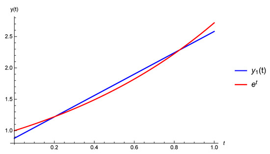
Figure 1. Comparison of approximate and exact solutions of System (12) for the case $r=2$ and $q=1$.

Table 1. Absolute errors in solution of System (12) with $r=2$ and $q=1$.

t	Error	t	Error
0.0	0.120825	0.5	0.08146
0.1	0.05579	0.6	0.07827
0.2	0.00182	0.7	0.05683
0.3	0.03992	0.8	0.01525
0.4	0.06816	0.9	0.04861

This is a degree 1 approximation, therefore $\mu =1$. Further, $M={max}_{[0,1]}{y}^{\prime }\left(t\right)=e$. The error estimate is obtained by using (11) is $M/2^4\approxeq 0.169893$. It can be checked from Table 1 that our computed values are less than this error bound.

Case 2: Now, we consider $r=3$ and $q=4$. A $12\times 12$ matrix K is given by:

$$\begin{array}{ccc}\hfill K& =& \left(\begin{array}{cccccc}1.0052& -0.1255& 0.0052& 0.7829& -0.0978& 0.0041\\ 0.1255& -0.0157& 0.0007& 0.0978& -0.0122& 0.0005\\ 0.0052& -0.0007& 0.0& 0.00401& -0.0005& 0.0\\ 1.2907& -0.1612& 0.0067& 1.0052& -0.1255& 0.0052\\ 0.1612& -0.0202& 0.0008& 0.1255& -0.0157& 0.0007\\ 0.0067& -0.0008& 0.0& 0.0052& -0.0007& 0.0\\ 1.6573& -0.2070& 0.0086& 1.2907& -0.1612& 0.0067\\ 0.2070& -0.0258& 0.0011& 0.1612& -0.0201& 0.0008\\ 0.0086& -0.0011& 0.0& 0.0067& -0.0008& 0.0\\ 2.1281& -0.2658& 0.0111& 1.6573& -0.2070& 0.0086\\ 0.2657& -0.0332& 0.0014& 0.2070& -0.0258& 0.0011\\ 0.0111& -0.0014& 0.0& 0.0086& -0.0011& 0.0\end{array}\right.\hfill \\ \hfill \end{array}$$

$$\begin{array}{c}\left.\begin{array}{cccccc}0.6097& -0.0761& 0.0032& 0.4748& -0.0593& 0.0025\\ 0.0761& -0.0095& 0.0003& 0.0593& -0.0074& 0.0003\\ 0.0032& -0.0004& 0.0& 0.0025& -0.0003& 0.0\\ 0.7829& -0.0978& 0.0040& 0.6097& -0.0761& 0.0032\\ 0.0978& -0.0122& 0.0005& 0.0761& -0.0095& 0.0004\\ 0.0041& -0.0005& 0.0& 0.0032& -0.0004& 0.0\\ 1.0052& -0.1255& 0.0052& 0.7829& -0.0978& 0.00401\\ 0.1255& -0.0157& 0.0007& 0.0978& -0.0122& 0.0005\\ 0.0052& -0.0007& 0.0& 0.0041& -0.0005& 0.0\\ 1.2907& -0.1612& 0.0067& 1.0052& -0.1255& 0.0052\\ 0.1612& -0.0201& 0.0008& 0.1255& -0.0157& 0.0007\\ 0.0067& -0.0008& 0.0& 0.0052& -0.0007& 0.0\end{array}\right)\hfill \end{array}$$

Other approximations in this case are as below:

$$\begin{array}{ccc}\hfill B\left(t\right)& =& \left({\chi }_{[0,1/4)},(-1+8t){\chi }_{[0,1/4)},(1-24t+96t^2){\chi }_{[0,1/4)},{\chi }_{[1/4,1/2)},\right.\hfill \\ & & (-3+8t){\chi }_{[1/4,1/2)},(13-72t+96t^2){\chi }_{[1/4,1/2)},{\chi }_{[1/2,3/4)},(-5+8t){\chi }_{[1/2,3/4)},\hfill \\ & & \left.(37-120t+96t^2){\chi }_{[1/2,3/4)},{\chi }_{[3/4,1)},(-7+8t){\chi }_{[3/4,1)},(73-168t+96t^2){\chi }_{[3/4,1)}\right),\hfill \end{array}$$

(where ${\chi }_A$ is the characteristic function of a set A)

$$\begin{array}{ccc}\hfill F& =& \left(3.08824,0.385629,0.0160607,3.96538,0.495157,0.0206224,\right.\hfill \\ & & {\left.5.09165,0.635795,0.0264796,6.53781,0.816377,0.0340005\right)}^T,\hfill \end{array}$$

$$Y_0={\left(1,0,0,1,0,0,1,0,0,1,0,0\right)}^T,$$

and

$$\begin{array}{ccc}\hfill Y& =& \left(1.1361,0.141865,0.00590841,1.45878,0.182158,0.00758655,\right.\hfill \\ & & {\left.1.87312,0.233896,0.00974132,2.40513,0.300328,0.0125081\right)}^T.\hfill \end{array}$$

The approximate solution of (12) is given by

$$\begin{array}{ccc}\hfill y_2\left(t\right)& =& 1.1361{\chi }_{[0,1/4)}+1.45878{\chi }_{[1/4,1/2)}+1.87312{\chi }_{[1/2,3/4)}+2.40513{\chi }_{[3/4,1)}\hfill \\ & & +0.3(-7+8t){\chi }_{[3/4,1)}+0.233896(-5+8t){\chi }_{[1/2,3/4)}\hfill \\ & & +0.182158(-3+8t){\chi }_{[1/4,1/2)}+0.14187(-1+8t){\chi }_{[0,1/4)}\hfill \\ & & +0.0125(73-168t+96t^2){\chi }_{[3/4,1)}+0.0097(37-120t+96t^2){\chi }_{[1/2,3/4)}\hfill \\ & & +0.00759(13-72t+96t^2){\chi }_{[1/4,1/2)}+0.00591(1-24t+96t^2){\chi }_{[0,1/4)}.\hfill \end{array}$$

Figure 2 shows the graphs of the approximate solution $y_2\left(t\right)$ and the exact solution $e^t$. The absolute errors at various values of t are given in Table 2. It can be observed that, in this case, the approximate solution is well in agreement with the exact solution. Further, using (11), the error bound is $0.01416$. Table 2 shows that our computed maximum value is $0.000145961$.

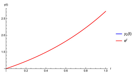
Figure 2. Comparison of approximate and exact solutions of System (12) for the case $r=3$ and $q=4$.

Table 2. Absolute errors in solution of System (12) with $r=3$ and $q=4$.

t	Error	t	Error
0.0	0.000145961	0.5	0.000240649
0.1	0.0000409679	0.6	0.0000675446
0.2	0.0000553281	0.7	0.0000912206
0.3	0.0000656897	0.8	0.000108304
0.4	0.0000536172	0.9	0.0000883998

Example 2.

Consider the following Volterra integro-differential system

$$\begin{array}{c}\hfill \left\{\begin{array}{c}y\left(t\right)+{\int }_0^{t}sin(t-s)y\left(s\right)y^{{}^{\prime }}\left(s\right)ds=2t^3+t^2-12t+12sin\left(t\right),\hfill \\ y\left(0\right)=0.\hfill \end{array}\right.\end{array}$$

(13)

Comparing with the standard form of System (4), we get $\beta =1,$$g(t,s)=sin(t-s)$, $m=0,$$n=1$, $f\left(t\right)=2t^3+t^2-12t+12sin\left(t\right)$, $l=0$ and $a_0=0$. We take $r=3$ and $q=4$. Following the procedure described in Section 2, we get

$$\begin{array}{ccc}\hfill F& =& \left(0.0208496,0.0312848,0.0104457,0.146854,0.0951443,0.0109877,\right.\hfill \\ & & {\left.0.406543,0.166108,0.0129514,0.824576,0.255306,0.0171862\right)}^T,\hfill \end{array}$$

$$\begin{array}{ccc}\hfill G& =& \left(\begin{array}{cccccc}0& -0.1245& 0& -0.2461& -0.1206& 0.0013\\ 0.1245& 0& -0.0006& 0.1206& -0.0039& -0.0006\\ 0& 0.0006& 0& 0.0013& 0.0006& 0\\ 0.2461& -0.1206& -0.0013& 0& -0.1245& 0\\ 0.1206& 0.0039& -0.0006& 0.1245& 0& -0.0006\\ -0.0013& 0.0006& 0& 0& 0.0006& 0\\ 0.4769& -0.1092& -0.0025& 0.2461& -0.1206& -0.0013\\ 0.1092& 0.0075& -0.0006& 0.1206& 0.0039& -0.0006\\ -0.0025& 0.0006& 0& -0.0013& 0.0006& 0\\ 0.6781& -0.0911& -0.0035& 0.4769& -0.1092& -0.0025\\ 0.0911& 0.0106& -0.0005& 0.1092& 0.0075& -0.0006\\ -0.0035& 0.0005& 0& -0.0025& 0.0006& 0\end{array}\right.\hfill \\ \hfill \end{array}$$

$$\begin{array}{c}\left.\begin{array}{cccccc}-0.4769& -0.1092& 0.0025& -0.6781& -0.0911& 0.0035\\ 0.1092& -0.0075& -0.0006& 0.0912& -0.0106& -0.0005\\ 0.0025& 0.0006& 0& 0.0035& 0.0005& 0\\ -0.2461& -0.1206& 0.0013& -0.4769& -0.1092& 0.0025\\ 0.1206& -0.0039& -0.0006& 0.1092& -0.0075& -0.0006\\ 0.0013& 0.0006& 0& 0.0025& 0.0006& 0\\ 0& -0.1245& 0& -0.2461& -0.1206& 0.0013\\ 0.1245& 0& -0.0006& 0.1206& -0.0039& -0.0006\\ 0& 0.0006& 0& 0.0013& 0.0006& 0\\ 0.2461& -0.1206& -0.00128& 0& -0.1245& 0\\ 0.1206& 0.0039& -0.0006& 0.1245& 0& -0.0006\\ -0.0013& 0.0006& 0& 0& 0.0006& 0\end{array}\right),\hfill \end{array}$$

$$Y_0={\left(0,0,0,0,0,0,0,0,0,0,0,0\right)}^T,$$

and $B\left(t\right)$ is same as given in the previous example. Using Equation (8), we get

$$\begin{array}{ccc}\hfill Y& =& \left(0.0208333,0.0312487,0.0104375,0.145833,0.0937492,0.0104781,\right.\hfill \\ & & {\left.0.395833,0.15625,0.0105145,0.770834,0.218753,0.010543\right)}^T.\hfill \end{array}$$

The approximate solution of System (13) is given by

$$\begin{array}{ccc}\hfill y_2\left(t\right)& =& 0.0208333{\chi }_{[0,1/4)}+0.145833{\chi }_{[1/4,1/2)}\hfill \\ & & +0.395833{\chi }_{[1/2,3/4)}+0.770834{\chi }_{[3/4,1)}\hfill \\ & & +0.218753(-7+8t){\chi }_{[3/4,1)}+0.15625(-5+8t){\chi }_{[1/2,3/4)}\hfill \\ & & +0.0937492(-3+8t){\chi }_{[1/4,1/2)}+0.0312487(-1+8t){\chi }_{[0,1/4)}\hfill \\ & & +0.010543(73-168t+96t^2){\chi }_{[3/4,1)}+0.0105145(37-120t+96t^2){\chi }_{[1/2,3/4)}\hfill \\ & & +0.0104781(13-72t+96t^2){\chi }_{[1/4,1/2)}+0.0104375(1-24t+96t^2){\chi }_{[0,1/4)}.\hfill \end{array}$$

The approximate solution $y_2\left(t\right)$ is compared with the exact solution $t^2$ in Figure 3. Table 3 shows the absolute error in the solution at different values of t.

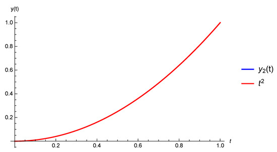
Figure 3. Comparison of approximate and exact solutions of System (13) for the case $r=3$ and $q=4$.

Table 3. Absolute errors in solution of System (13) with $r=3$ and $q=4$.

t	Error	t	Error
0.0	0.0000221689	0.5	0.0000975226
0.1	8.9 $\times {10}^{-6}$	0.6	0.0000429716
0.2	4.99 $\times {10}^{-8}$	0.7	4.32 $\times {10}^{-6}$
0.3	3 $\times {10}^{-6}$	0.8	3.76 $\times {10}^{-6}$
0.4	0.0000271471	0.9	0.0000547743

Using (11), the error-bound for this example is approximately $0.0104167$ and our value from Table 3 is $0.0000271471$.

Comparison with Other Methods

In this section, we compare our results with the existing methods viz. Daftardar–Gejji–Jafari (DGJ) method [33], Adomian decomposition method (ADM) [34] and quadrature methods [35,36].

The DGJ algorithm for the solution of Equation (12) is $y_0=e^{t+1}$ and $y_{n+1}=y_0-{\int }_0^1{e}^{t-s}{y}_n\left(s\right)y_n^{{}^{\prime }}\left(s\right)ds,$$n=0,1,2,\cdots$. The k-term approximate solution is given by $y_{k-1}$. Therefore, the three-term solution is $y\left(t\right)=e^{(1+t)}\left(1-(-1+e)e{(1+e-e^2)}^2\right)$.

The ADM algorithm for the solution of Equation (12) is $y_0=e^{t+1}$ and $y_{n+1}=-{\int }_0^1{e}^{t-s}\frac{1}{2}\frac{d{A}_n\left(s\right)}{ds}ds,$$n=0,1,2,\cdots ,$ where $A_n\left(s\right)$ are the Adomian polynomials [34] of the function $y^2\left(s\right)$. The k-term approximate solution using ADM is given by ${\sum }_{n=0}^{k-1}{y}_n$. Therefore, the three-term solution is $y\left(t\right)=e^{(1+t)}\left(1+e+e^2-4e^3+2e^4\right)$.

The comparison of these solutions with the exact solution in Figure 4 shows that these methods diverge for this example.

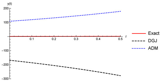
Figure 4. Comparison of DGJ, ADM and exact solutions of System (12).

Let us divide the interval $[0,1]$ into n equal sub-intervals of length h. The approximation of the function y at the node $jh$ is denoted by $y_j$. We take n as an even natural number. The Simpson’s quadrature numerical algorithm [36] applied to Equation (12) provides the following expression:

$$y_j=\frac{1}{2}(e+1)e^{jh}-\frac{h}{6}\left(e^{jh}{y}_0^2+4\sum _{k=1}^{n/2}{e}^{(j-2k+1)h}{y}_{2k-1}^2+2\sum _{k=1}^{n/2-1}{e}^{(j-2k)h}{y}_{2k}^2+e^{(j-n)h}{y}_n^2\right),$$

(14)

where $y_0=1$ and $j=1,2,\cdots ,n$. This algorithm provides the solution which is in agreement with the exact solution. We compare the absolute errors at various points with $h=0.05$ and $n=20$ in Table 4.

Table 4. Absolute errors in the solution of System (12) with quadrature method and $h=0.05$, $n=20$.

t	Error	t	Error
0.0	0	0.5	0.0214405
0.1	0.014372	0.6	0.0236955
0.2	0.0158835	0.7	0.0261875
0.3	0.017554	0.8	0.0289417
0.4	0.0194002	0.9	0.0319855

It can be observed from Table 2 and Table 4 that our method has less error as compared with quadrature method.

Similarly, we compare our results of Equation (13) with DGJ, ADM and trapezium quadrature rule.

The 2-term approximate solutions of this example using DGJ and ADM provide the same expression given by $y\left(t\right)=-312-2160t+157t^2+336t^3-10t^4-12t^5+3(104-15t+t^2+2t^3)cos\left(t\right)+(2157-3t+27t^2-2t^3-3t^4)sin\left(t\right)+24sin\left(2t\right)$.

As in Equation (12), we divide the interval $[0,1]$ into n equal intervals, where n is a natural number. The trapezium quadrature formula to compute the solution of Equation (13) is

$$y_j=u_j-\frac{h}{4}\left(y_j^2+cos\left(jh\right)y_0^2+2\sum _{k=1}^{j-1}cos\left((j-k)h\right)y_k^2\right),$$

where $u_j=2{\left(jh\right)}^3+{\left(jh\right)}^2-12jh+12sin\left(jh\right)$ and $y_0=0$. We take $h=0.05$ and $n=20$.

It is observed that all these methods provide the solutions which are matching with the exact solution. We compare the absolute errors in these solutions at various points in Table 5.

Table 5. Absolute errors in solutions of System (13) obtained by using DGJ/ADM and quadrature method.

t	DGJ/ADM Error	Quadrature Rule Error	t	DGJ/ADM Error	Quadrature Rule Error
0.0	0	0	0.5	0.0000486807	0.0000509481
0.1	1.24837$\times {10}^{-10}$	4.06185$\times {10}^{-7}$	0.6	0.000209306	0.0000867569
0.2	3.19707$\times {10}^{-8}$	3.30782$\times {10}^{-6}$	0.7	0.000718813	0.000134977
0.3	8.18704$\times {10}^{-7}$	0.0000111665	0.8	0.00209495	0.000196122
0.4	8.17149$\times {10}^{-6}$	0.0000263365	0.9	0.00538832	0.000269884

It is observed that the error in our method is smaller at most of the points.

6. Conclusions

In this work, we have discussed an efficient method for solving a class of Fredholm and Volterra integro-differential equations. Our method is based on a new approximation for the derivatives of the equations’ solutions using hybrid and block-pulse functions. The absolute errors reported in tables show that the approximate solution is in a good agreement with the exact solution. It is verified in each example that the practical error in our method is less than the theoretical error-bound. In fact, this method is highly efficient, very easy and a powerful mathematical tool for finding the numerical solution of some class of Fredholm and Volterra integro-differential equations. The approximate solutions are found by using the computer code written in Wolfram Mathematica. The method is computationally attractive, and applications are demonstrated through illustrative examples. For future research works, we can use this method to solve various kinds of problems such as higher dimensional problems, stochastic integro-differential equations and partial integro-differential equations of fractional order with additional work. The comparison with other methods viz. DGJ, ADM and quadrature rules shows that our method works equally well for Fredholm as well as Volterra equations and produce the results with a smaller error.

References

- Bloom, F. Asymptotic bounds for solutions to a system of damped integro-differential equations of electromagnetic theory. J. Math. Anal. Appl. 1980, 73, 524–542. [Google Scholar] [CrossRef]
- Holmaker, K. Global asymptotic stability for a stationary solution of a system of integro-differential equations describing the formation of liver zones. SIAM J. Math. Anal. 1993, 24, 116–128. [Google Scholar] [CrossRef]
- Abdou, M.A. On asymptotic methods for Fredholm–Volterra integral equation of the second kind in contact problems. J. Comput. Appl. Math. 2003, 154, 431–446. [Google Scholar] [CrossRef]
- Forbes, L.K.; Crozier, S.; Doddrell, D.M. Calculating current densities and fields produced by shielded magnetic resonance imaging probes. SIAM J. Appl. Math. 1997, 57, 401–425. [Google Scholar]
- Delves, L.M.; Mohamed, J.L. Computational Methods for Integral Equations; Cambridge University Press: Cambridge, UK, 1985. [Google Scholar]
- Basirat, B.; Maleknejad, K.; Hashemizadeh, E. Operational matrix approach for the nonlinear Volterra–Fredholm integral equations: Arising in physics and engineering. Int. J. Phys. Sci. 2012, 7, 226–233. [Google Scholar]
- Wazwaz, A.M. A First Course in Integral Equations; World Scientifics: Singapore, 1997. [Google Scholar]
- Polyanin, A.D.; Manzhirov, A.V. Handbook of Integral Equations, 2nd ed.; Chapman and Hall/CRC Press: London, UK, 2008. [Google Scholar]
- Golberg, M.A. The convergence of a collocations method for a class of Cauchy singular integral equations. J. Math. Appl. 1984, 100, 500–512. [Google Scholar] [CrossRef]
- Kovalenko, E.V. Some approximate methods for solving integral equations of mixed problems. Probl. Math. Mech. 1989, 53, 85–92. [Google Scholar] [CrossRef]
- Semetanian, B.J. On an integral equation for axially symmetric problem in the case of an elastic body containing an inclusion. J. Appl. Math. Mech. 1991, 55, 371–375. [Google Scholar] [CrossRef]
- Willis, J.R.; Nemat-Nasser, S. Singular perturbation solution of a class of singular integral equations. Quart. Appl. Math. 1990, XLVIII, 741–753. [Google Scholar] [CrossRef][Green Version]
- Frankel, J. A Galerkin solution to regularized Cauchy singular integro-differential equation. Q. Appl. Math. 1995, 52, 145–258. [Google Scholar] [CrossRef]
- Golbabai, A.; Javidi, M. Application of He’s homotopy perturbation method for nth-order integro-differential equations. Appl. Math. Comput. 2007, 190, 1409–1416. [Google Scholar] [CrossRef]
- Shang, X.; Han, D. Application of the variational iteration method for solving nth-order integro-differential equations. J. Comput. Appl. Math. 2010, 234, 1442–1447. [Google Scholar] [CrossRef]
- Abbasbandy, S.; Shivanian, E. Application of variational iteration method for nth-order integro-differential equations. Zeitschrift fur Naturforschung A 2009, 64, 439–444. [Google Scholar] [CrossRef]
- Hou, J.; Yang, C. Numerical method in solving Fredholm integro-differential equations by using hybrid function operational matrix of derivative. J. Inf. Comput. Sci. 2013, 10, 2757–2764. [Google Scholar] [CrossRef]
- Hemeda, A.A. New iterative method: Application to nth-order integro-differential equations. Int. Math. Forum 2012, 7, 2317–2332. [Google Scholar]
- Daftardar-Gejji, V.; Jafari, H. An iterative method for solving non-linear functional equations. J. Math. Anal. Appl. 2006, 316, 753–763. [Google Scholar] [CrossRef]
- Marzban, H.R.; Razzaghi, M. Optimal control of linear delay systems via hybrid of block-pulse and Legendre polynomials. J. Franklin Inst. 2004, 341, 279–293. [Google Scholar] [CrossRef]
- Razzaghi, M.; Marzban, H.R. A hybrid analysis direct method in the calculus of variations. Int. J. Comput. Math. 2000, 75, 259–269. [Google Scholar] [CrossRef]
- Hsiao, C.H. Hybrid function method for solving Fredholm and Volterra integral equations of the second kind. J. Comput. Appl. Math. 2009, 230, 59–68. [Google Scholar] [CrossRef]
- Maleknejad, K.; Basirat, B.; Hashemizadeh, E. Hybrid Legendre polynomials and block-pulse functions approach for nonlinear Volterra–Fredholm integro-differential equations. Comput. Math. Appl. 2011, 61, 282–288. [Google Scholar] [CrossRef]
- Mizaee, F. Numerical solution of system of linear integral equations via improvement of block-pulse functions. J. Math. Model. 2016, 4, 133–159. [Google Scholar]
- Mizaee, F.; Alipour, S. Approximate solution of nonlinear quadratic integral equations of fractional order via piecewise linear functions. J. Comput. Appl. Math. 2018, 331, 217–227. [Google Scholar] [CrossRef]
- Mizaee, F.; Alipour, S.; Samadyar, N. Numerical solution based on hybrid of block-pulse and parabolic functions for solving a system of nonlinear stochastic Ito–Volterra integral equations of fractional order. J. Comput. Appl. Math. 2019, 349, 157–171. [Google Scholar] [CrossRef]
- Mizaee, F.; Hoseini, S.F. A new collocation approach for solving systems of high-order linear Volterra integro-differential equations with variable coefficients. Appl. Math. Comput. 2017, 311, 272–282. [Google Scholar]
- Mizaee, F.; Hoseini, S.F. Hybrid functions of Bernstein polynomials and block-pulse functions for solving optimal control of the nonlinear Volterra integral equations. Indag. Math. 2016, 27, 835–849. [Google Scholar] [CrossRef]
- Hashemizadeh, E.; Basirat, B. An efficient computational method for the system of linear Volterra integral equations by means of hybrid functions. Math. Sci. 2011, 5, 355–368. [Google Scholar]
- Shojaeizadeh, T.; Abadi, Z.; Golpar Raboky, E. Hybrid functions approach for solving Fredholm and Volterra integral equations. J. Prime Res. Math. 2009, 5, 124–132. [Google Scholar]
- Which Method Does Mathematica Use in NSolve for One Variable Functions? Available online: https://community.wolfram.com/groups/-/m/t/116219 (accessed on 22 May 2020).
- Stewart, G.W. Afternotes on Numerical Analysis; SIAM: Philadelphia, PA, USA, 1996; Volume 49. [Google Scholar]
- Kumar, M.; Jhinga, A.; Daftardar-Gejji, V. New algorithm for solving non-linear functional equations. Int. J. Appl. Comput. Math. 2020, 6, 26. [Google Scholar] [CrossRef]
- Adomian, G. Solving Frontier Problems of Physics: The Decomposition Method; Springer Science and Business Media: Dordrecht, The Netherlands, 2013; Volume 60. [Google Scholar]
- Van der Houwen, P.J.; Wolkenfelt, P.H.M. On the stability of multistep formulas for Volterra integral equations of the second kind. Computing 1980, 24, 341–347. [Google Scholar] [CrossRef]
- Ray, S.S.; Sahu, P.K. Numerical methods for solving Fredholm integral equations of second kind. Abstr. Appl. Anal. 2013, 2013, 426916. [Google Scholar] [CrossRef]
© 2020 by the authors. Licensee MDPI, Basel, Switzerland. This article is an open access article distributed under the terms and conditions of the Creative Commons Attribution (CC BY) license (http://creativecommons.org/licenses/by/4.0/).