Modified Potra–Pták Multi-step Schemes with Accelerated Order of Convergence for Solving Systems of Nonlinear Equations

Abstract

In this study, an iterative scheme of sixth order of convergence for solving systems of nonlinear equations is presented. The scheme is composed of three steps, of which the first two steps are that of third order Potra–Pták method and last is weighted-Newton step. Furthermore, we generalize our work to derive a family of multi-step iterative methods with order of convergence $3r+6,r=0,1,2,\dots .$ The sixth order method is the special case of this multi-step scheme for $r=0.$ The family gives a four-step ninth order method for $r=1.$ As much higher order methods are not used in practice, so we study sixth and ninth order methods in detail. Numerical examples are included to confirm theoretical results and to compare the methods with some existing ones. Different numerical tests, containing academical functions and systems resulting from the discretization of boundary problems, are introduced to show the efficiency and reliability of the proposed methods.

1. Introduction

Many applied problems in Science and Engineering [1,2,3] are reduced to solve nonlinear systems $F(x)=0$ numerically, that is, for a given nonlinear function $F(x):D\subset R^m⟶R^m$, where $F(x)={(f_1(x),f_2(x),\dots ,f_m(x))}^T$ and $x={(x_1,x_2,\dots ,x_m)}^T$, to find a vector $\alpha ={({\alpha }_1,{\alpha }_2,\dots ,{\alpha }_m)}^T$ such that $F(\alpha )=0.$ The most widely used method for this purpose is the classical Newton’s method [3,4], which converges quadratically under the conditions that the function F is continuously differentiable and a good initial approximation $x^{(0)}$ is given. It is defined by

$$x^{(k+1)}=x^{(k)}-F^{\prime }{(x^{(k)})}^{-1}F(x^{(k)}),k=0,1,\dots ,$$

(1)

where $F^{\prime }{(x^{(k)})}^{-1}$ is the inverse of Fréchet derivative $F^{\prime }(x^{(k)})$ of the function $F(x)$ at $x^{(k)}$. In order to improve the order of convergence of Newton’s method, several methods have been proposed in literature, see, for example [5,6,7,8,9,10,11] and references therein. In particular, the third order method by Potra–Pták [11] for systems of nonlinear equations is given by

$$\begin{array}{ccc}\hfill y^{(k)}& =& x^{(k)}-F^{\prime }{(x^{(k)})}^{-1}F(x^{(k)}),\hfill \\ \hfill x^{(k+1)}& =& y^{(k)}-F^{\prime }{(x^{(k)})}^{-1}F(y^{(k)})k=0,1,\dots \hfill \end{array}$$

(2)

It is quite clear that this scheme requires the evaluation of two functions, one derivative and one matrix inversion per iteration, that is usually avoided by solving a linear system. This algorithm is illustrious not only for its simplicity but also for its efficient character.

In this paper, based on Potra–Pták method (2), we develop a three-step scheme with increased order of convergence and still maintaining the efficient character. With these considerations, we propose a three-step iterative method with accelerated sixth order of convergence; of the three steps, the first two are those of Potra–Pták method whereas the third is a weighted Newton-step. Then, based on this scheme, a multi-step family with increasing order of convergence $3r+6,r=0,1,2,\dots ,$ is developed. The sixth order method is the special case of this multi-step scheme for $r=0.$ The family gives a four-step ninth order scheme for $r=1.$ As much higher order methods are not used in practice, so we study sixth and ninth order methods in particular.

The rest of the paper is organized as follows: In Section 2, we present the new three-step scheme for solving nonlinear systems and we analyze its order of convergence. In Section 2.1, the order of this scheme is improved in three units, by adding another step that needs a new functional evaluation and to solve a linear system with the same matrix of coefficients as before. This idea can be generalized for designing an iterative method with arbitrary order of convergence. The computational efficiency of the proposed schemes is studied in Section 3, doing a comparative analysis with the efficiency of other known methods. Section 4 is devoted to the numerical experiments with academical multivariate functions and nonlinear systems resulted of the discretization of boundary problems. For some cases, the basins of attraction of the methods are also showed. The paper finishes with some conclusions and the references used in it.

2. The Method and Analysis of Convergence

We start with the following iterative scheme:

$$\begin{array}{ccc}\hfill y^{(k)}& =& x^{(k)}-F^{\prime }{(x^{(k)})}^{-1}F(x^{(k)}),\hfill \\ \hfill z^{(k)}& =& y^{(k)}-F^{\prime }{(x^{(k)})}^{-1}F(y^{(k)}),\hfill \\ \hfill x^{(k+1)}& =& z^{(k)}-(aI+F^{\prime }{(x^{(k)})}^{-1}[z^{(k)},y^{(k)};F](bI+c{F}^{\prime }{(x^{(k)})}^{-1}[z^{(k)},y^{(k)};F]))F^{\prime }{(x^{(k)})}^{-1}F(z^{(k)}),\hfill \end{array}$$

(3)

where the first two-steps are those of Potra–Pták scheme [11] for nonlinear systems and $[z^{(k)},y^{(k)};F]$ is the first order divided difference of F.

In order to discuss the behavior of scheme (3), we consider the following expression of divided difference operator $[·,·;F]:D\times D\subset R^m\times R^m⟶L(R^m)$, see for example, [2,10],

$$[x+h,x;F]={\int }_0^1{F}^{\prime }(x+th)dt,\forall x,h\in R^m.$$

(4)

By expanding $F^{\prime }(x+th)$ in Taylor series at the point x and integrating, we have

$$[x+h,x;F]={\int }_0^1{F}^{\prime }(x+th)dt=F^{\prime }(x)+\frac{1}{2}{F}^{″}(x)h+\frac{1}{6}{F}^{″}(x)h^2+O(h^3).$$

(5)

where $h^i=(h,h,\stackrel{i}{\dots },h),h\in R^m.$ Let $e^{(k)}=x^{(k)}-\alpha$. Developing $F(x^{(k)})$ in a neighborhood of $\alpha$ and assuming that $\Gamma ={[F^{\prime }(\alpha )]}^{-1}$ exists, we have

$$F(x^{(k)})=F^{\prime }(\alpha )(e^{(k)}+A_2{(e^{(k)})}^2+A_3{(e^{(k)})}^3+A_4{(e^{(k)})}^4+O({(e^{(k)})}^5)),$$

(6)

where $A_i=\frac{1}{i!}\Gamma F^{(i)}(\alpha )\in L_i(R^m,R^m)$ and ${(e^{(k)})}^i=(e^{(k)},e^{(k)},\stackrel{i}{\dots },e^{(k)}),e^{(k)}\in R^m$. Also,

$$F^{\prime }(x^{(k)})=F^{\prime }(\alpha )(I+2A_2{e}^{(k)}+3A_3{(e^{(k)})}^2+4A_4{(e^{(k)})}^3+O({(e^{(k)})}^4)),$$

(7)

$$F^{″}(x^{(k)})=F^{\prime }(\alpha )(2A_2+6A_3{e}^{(k)}+12A_4{(e^{(k)})}^2+O({(e^{(k)})}^3)),$$

(8)

$$F^{″}(x^{(k)})=F^{\prime }(\alpha )(6A_3+24A_4{e}^{(k)}+O({(e^{(k)})}^2)).$$

(9)

Inversion of $F^{\prime }(x^{(k)})$ yields,

$$F^{\prime }{(x^{(k)})}^{-1}=\left[I-2A_2{e}^{(k)}+(4A_2^2-3A_3){(e^{(k)})}^2-(8A_2^3-6A_2{A}_3-6A_3{A}_2+4A_4){(e^{(k)})}^3+O({(e^{(k)})}^4)\right]\Gamma .$$

(10)

We are in a position to analyze the behavior of scheme (3). Thus, the following result is proven.

Theorem 1.

Let $F:D\subset R^m\to D$ be sufficiently differentiable function in an open neighborhood D of its zero α. Let us suppose that the Jacobian matrix $F^{\prime }(x)$ is continuous and nonsingular at α. If an initial approximation $x^{(0)}$ is sufficiently close to α, then the local order of convergence of method (3) is at least $6,$ provided $a=13/4,b=-7/2$ and $c=5/4.$

Proof. 

Let $e_y^{(k)}=y^{(k)}-\alpha$ is the local error of Newton’s method given by

$$e_y^{(k)}=A_2{(e^{(k)})}^2-2(A_2^2-A_3){(e^{(k)})}^3+O({(e^{(k)})}^4).$$

(11)

Employing Equations (10) and (11) in the second step of (3), we get

$$e_z^{(k)}=z^{(k)}-\alpha =2A_2{e}^{(k)}{e}_y^{(k)}+O({(e^{(k)})}^4).$$

(12)

Using Equations (7)–(9) in (5) for $x+h=z^{(k)}$, $x=y^{(k)}$ and $h=e_z^{(k)}-e_y^{(k)}$, it follows that

$$[z^{(k)},y^{(k)};F]=F^{\prime }(\alpha )(I+A_2(e_y^{(k)}+e_z^{(k)})+O({(e^{(k)})}^4)).$$

(13)

With the help of Equations (10) and (13), we can write

$$\begin{array}{cc}\hfill aI+& F^{\prime }{(x^{(k)})}^{-1}[z^{(k)},y^{(k)};F](bI+c{F}^{\prime }{(x^{(k)})}^{-1}[z^{(k)},y^{(k)};F])\hfill \\ & =\left[(a+b+c)I-2(b+2c)A_2{e}^{(k)}+((5b+14c)A_2^2-3(b+2c)A_3){(e^{(k)})}^2-(10(b+4c)A_2^3\right.\hfill \\ & \left.-(8b+22c)A_2{A}_3-(6b+18c)A_3{A}_2+4(b+2c)A_4){(e^{(k)})}^3+O({(e^{(k)})}^4)\right]\Gamma .\hfill \end{array}$$

(14)

Expanding $F(z^{(k)})$ about $\alpha$, we obtain

$$F(z^{(k)})=F^{\prime }(\alpha )\left(e_z^{(k)}+A_2{(e_z^{(k)})}^2+O({(e_z^{(k)})}^3)\right).$$

(15)

Using (10), (14) and (15) in the last step of (3), we get

$$\begin{array}{cc}\hfill e^{(k+1)}=& x^{(k+1)}-\alpha =2\left(1-a-b-c\right)A_2^2{(e^{(k)})}^3+4(a+2b+3c)A_2^3{(e^{(k)})}^4\hfill \\ & -2((4a+13(b+2c))A_2^2-3A_3(a+2b+3c))A_2^2{(e^{(k)})}^5+4((3a+17b+45c)A_2^5\hfill \\ & -(3a+10(b+2c))A_2{A}_3{A}_2^2+(3a+6(b+3c))A_3{A}_2^3+2(a+2b+3c)A_4{A}_2^2){(e^{(k)})}^6\hfill \\ & +O({(e^{(k)})}^7).\hfill \end{array}$$

(16)

In order to achieve sixth order of convergence it is clear that terms $1-a-b-c,$$a+2b+3c$ and $4a+13(b+2c)$ must vanish for some values of $a,$b, and c. This happens when $a=\frac{13}{4},$$b=-\frac{7}{2}$ and $c=\frac{5}{4}$. Thus, the error equation (16) becomes

$$\begin{array}{c}\hfill e^{(k+1)}=x^{(k+1)}-\alpha =(26A_2^3+A_2{A}_3-3A_3{A}_2)A_2^2{(e^{(k)})}^6+O({(e^{(k)})}^7).\end{array}$$

(17)

This proves the sixth order of convergence. □

Thus, the proposed scheme (3) is given by

$$\begin{array}{ccc}\hfill y^{(k)}& =& x^{(k)}-F^{\prime }{(x^{(k)})}^{-1}F(x^{(k)}),\hfill \\ \hfill z^{(k)}& =& y^{(k)}-F^{\prime }{(x^{(k)})}^{-1}F(y^{(k)}),\hfill \\ \hfill x^{(k+1)}& =& z^{(k)}-\left(\frac{13}{4}I-F^{\prime }{(x^{(k)})}^{-1}[z^{(k)},y^{(k)};F]\left(\frac{7}{2}I-\frac{5}{4}{F}^{\prime }{(x^{(k)})}^{-1}[z^{(k)},y^{(k)};F]\right)\right)\hfill \\ & & \times F^{\prime }{(x^{(k)})}^{-1}F(z^{(k)}).\hfill \end{array}$$

(18)

Clearly this formula uses three functional evaluations, one evaluation of the Jacobian matrix, one of a divided difference, and one matrix inversion per iteration. We denote this scheme by ${\mathrm{H}}_{6,1}.$

2.1. Multi-step Method with Order $3r+6$

In this section, we improve the ${\mathrm{H}}_{6,1}$ by adding a functional evaluation per each new step to get the multi-step version called ${\mathrm{H}}_{3r+6,1}$ method. The method is defined as

$$\begin{array}{ccc}\hfill x^{(k+1)}& =& {\mathrm{H}}_{3r+6,1}(x^{(k)})={\nu }_r(x^{(k)}),\hfill \\ \hfill {\nu }_j(x^{(k)})& =& {\nu }_{j-1}(x^{(k)})-\theta (x^{(k)})F^{\prime }{(x^{(k)})}^{-1}F({\nu }_{j-1}(x^{(k)})),\hfill \\ \hfill \theta (x^{(k)})& =& \frac{13}{4}I-F^{\prime }{(x^{(k)})}^{-1}[z^{(k)},y^{(k)};F]\left(\frac{7}{2}I-\frac{5}{4}{F}^{\prime }{(x^{(k)})}^{-1}[z^{(k)},y^{(k)};F]\right),\hfill \\ \hfill {\nu }_0& =& {\mathrm{H}}_{6,1}(x^{(k)}),j=1,2,\dots ,r;r⩾1.\hfill \end{array}$$

(19)

Let us note that case $r=0$ is ${\mathrm{H}}_{6,1}$ method given by (18). This multi-step version has the order of convergence $3r+6,r⩾1,$ which we shall prove through the following result.

Theorem 2.

Let us Assume that $F:D\subset {\mathbb{R}}^m⟶D$ is a sufficiently Fréchet differentiable function in an open convex set D containing the zero α of $F(x)$ and $F^{\prime }(x)$ is continuous and nonsingular at α. Then, sequence ${\left\{x^{(k)}\right\}}_{k⩾0}$, $x^{(0)}\in D$ obtained by using method (19) converges to α with convergence order $3r+6.$

Proof. 

Let $e_{{\nu }_j}^{(k)}={\nu }_j^{(k)}-\alpha ,$ for all $j=1,2,\dots ,r.$ Taylor’s expansion of $F({\nu }_{j-1}^{(k)}(x^{(k)}))$ about $\alpha$ yields

$$F({\nu }_{j-1}(x^{(k)}))=F^{\prime }(\alpha )\left(e_{{\nu }_{j-1}}^{(k)}+A_2{(e_{{\nu }_{j-1}}^{(k)})}^2+O({(e_{{\nu }_{j-1}}^{(k)})}^3)\right).$$

(20)

Using (10) and (14) for $a=13/4,b=-7/2$ and $c=5/4,$ we have

$$\begin{array}{cc}\hfill \theta (x^{(k)})F^{\prime }{(x^{(k)})}^{-1}=& \left(\frac{13}{4}I-F^{\prime }{(x^{(k)})}^{-1}[z^{(k)},y^{(k)};F]\left(\frac{7}{2}I-\frac{5}{4}{F}^{\prime }{(x^{(k)})}^{-1}[z^{(k)},y^{(k)};F]\right)\right)F^{\prime }{(x^{(k)})}^{-1}\hfill \\ \hfill =& \left[I-S_3{(e^{(k)})}^3+O({(e^{(k)})}^4)\right]\Gamma ,\hfill \end{array}$$

(21)

where $S_3=15A_2^3+\frac{1}{2}{A}_2{A}_3-\frac{3}{2}{A}_3{A}_2.$

With the help of (20) and (21), we can write

$$\begin{array}{cc}\hfill \theta (x^{(k)})F^{\prime }{(x^{(k)})}^{-1}F({\nu }_{j-1}(x^{(k)}))=& (I-S_3{(e^{(k)})}^2+\cdots )(e_{{\nu }_{j-1}}^{(k)}+A_2{(e_{{\nu }_{j-1}}^{(k)})}^2+\cdots )\hfill \\ \hfill =& e_{{\nu }_{j-1}}^{(k)}-S_3{(e^{(k)})}^3{e}_{{\nu }_{j-1}}^{(k)}+\cdots .\hfill \end{array}$$

(22)

By substituting (22) in (19), we get

$$\begin{array}{cc}\hfill e_{{\nu }_j}^{(k)}=& {\nu }_j^{(k)}-\alpha =e_{{\nu }_{j-1}}^{(k)}-(e_{{\nu }_{j-1}}^{(k)}-S_3{(e^{(k)})}^3{e}_{{\nu }_{j-1}}^{(k)}+\cdots )\hfill \\ \hfill =& S_3{(e^{(k)})}^3{e}_{{\nu }_{j-1}}^{(k)}+\cdots .\hfill \end{array}$$

(23)

As we know that $e_{{\nu }_0}^{(k)}=(26A_2^3+A_2{A}_3-3A_3{A}_2)A_2^2{(e^{(k)})}^6,$ so from (23), for $j=1,2,\dots ,$ we have that

$$\begin{array}{cc}\hfill e_{{\nu }_1}^{(k)}=& S_3{(e^{(k)})}^3{e}_{{\nu }_0}^{(k)}\hfill \\ \hfill =& S_3{(e^{(k)})}^3(26A_2^3+A_2{A}_3-3A_3{A}_2)A_2^2{(e^{(k)})}^6+\cdots ,\hfill \\ \hfill e_{{\nu }_2}^{(k)}=& S_3{(e^{(k)})}^2{e}_{{\nu }_1}^{(k)}\hfill \\ \hfill =& S_3^2{(e^{(k)})}^6(26A_2^3+A_2{A}_3-3A_3{A}_2)A_2^2{(e^{(k)})}^6+\cdots .\hfill \end{array}$$

(24)

Proceeding by induction, we have

$$e_{{\nu }_r}^{(k)}=S_3^r(26A_2^3+A_2{A}_3-3A_3{A}_2)A_2^2{(e^{(k)})}^{3r+6}+O({(e^{(k)})}^{3r+7}),r⩾0.$$

(25)

Hence, the result of the theorem is proven. □

As a special case, this family when $r=1$ gives a ninth order method:

$$\begin{array}{ccc}\hfill y^{(k)}& =& x^{(k)}-F^{\prime }{(x^{(k)})}^{-1}F(x^{(k)}),\hfill \\ \hfill z^{(k)}& =& x^{(k)}-F^{\prime }{(x^{(k)})}^{-1}F(y^{(k)}),\hfill \\ \hfill {\nu }_0^{(k)}& =& {\mathrm{H}}_{6,1}(x^{(k)},y^{(k)}),\hfill \\ \hfill x^{(k+1)}& =& {\nu }_0^{(k)}-\theta (x^{(k)})F^{\prime }{(x^{(k)})}^{-1}F({\nu }_0^{(k)})k=0,1,2,\dots \hfill \end{array}$$

(26)

It is clear that this scheme requires four functional evaluations, one Jacobian matrix, one divided difference, and one matrix inversion per full iteration. We denote this scheme by ${\mathrm{H}}_{9,1}.$

Remark 1.

Multi-step version $H_{3r+6}$$(r⩾0),$ utilizes $r+3$ functional evaluations of $F,$ one evaluation of $F^{\prime }$, and one divided difference. Also, the scheme (19) requires only one matrix inversion per iteration.

3. Computational Efficiency

To obtain an estimation of the efficiency of the proposed methods we shall make use of efficiency index, according to which the efficiency of an iterative method is given by $E={\rho }^{\frac{1}{C}}$, where $\rho$ is the order of convergence and C is the computational cost per iteration. For a system of m nonlinear equations and m unknowns, the computational cost per iteration is given by (see [9,10])

$$C({\mu }_0,{\mu }_1,m)=P_0(m){\mu }_0+P_1(m){\mu }_1+P(m),$$

(27)

where $P_0(m)$ represents the number of evaluations of scalar functions $(f_1,f_2,\dots ,f_m)$ used in the evaluations of F and $[y,x;F]$. The divided difference $[y,x;F]$ of F is an $m\times m$ matrix with elements (see [11,12])

$$\begin{array}{cc}\hfill {[y,x;F]}_{ij}=& (f_i(y_1,.....,y_{j-1},y_j,x_{j+1},.....,x_m)-f_i(y_1,.....,y_{j-1},x_j,x_{j+1},.....,x_m)\hfill \\ & +f_i(x_1,.....,x_{j-1},y_j,y_{j+1},.....,y_m)\hfill \\ & -f_i(x_1,.....,x_{j-1},x_j,y_{j+1},.....,y_m))/(2(y_j-x_j)),1⩽i,j⩽m.\hfill \end{array}$$

The number of evaluations of scalar functions of $F^{\prime }$, i.e. $\frac{\partial f_i}{\partial x_j}$, $1⩽i,j⩽m$, is $P_1(m)$. $P(m)$ represents the number of products or quotients needed per iteration, and ${\mu }_0$ and ${\mu }_1$ are ratios between products and evaluations required to express the value of $C({\mu }_0,{\mu }_1,m)$ in terms of products.

To compute F in any iterative method we calculate m scalar functions and if we compute the divided difference $[y,x;F]$ then we evaluate $2m(m-1)$ scalar functions, where $F(x)$ and $F(y)$ are computed separately. We must add $m^2$ quotients from any divided difference. The number of scalar evaluations is $m^2$ for any new derivative $F^{\prime }$. In order to compute an inverse linear operator we solve a linear system, where we have $m(m-1)(2m-1)/6$ products and $m(m-1)/2$ quotients in the LU decomposition and $m(m-1)$ products and m quotients in the resolution of two triangular linear systems. We suppose that a quotient is equivalent to l products. Moreover, we add $m^2$ products for the multiplication of a matrix with a vector or of a matrix by a scalar and m products for the multiplication of a vector by a scalar.

Denoting the efficiency indices of ${\mathrm{H}}_{\rho ,i}$ ($\rho =6,9$ and $i=1,2,3,4$) by $E_{\rho ,i}$ and computational cost by $C_{\rho ,i}$, then taking into account the above considerations, we obtain

$$C_{6,1}=(2m^2+m){\mu }_0+m^2{\mu }_1+\frac{m}{6}(2m^2+39m-11+9l(m+3))and{E}_{6,1}=6^{1/C_{6,1}}.$$

(28)

$$C_{9,1}=(2m^2+2m){\mu }_0+m^2{\mu }_1+\frac{m}{6}(2m^2+69m-11+9l(m+5))and{E}_{9,1}=9^{1/C_{9,1}}.$$

(29)

To check the performance of the new sixth order method, we compare it with some existing sixth order which belongs to the same class. So, we choose the sixth order methods presented in [10,13]. The sixth order methods presented in [10] are given by

$$\begin{array}{ccc}\hfill y^{(k)}& =& x^{(k)}-F^{\prime }{(x^{(k)})}^{-1}F(x^{(k)}),k=0,1,2,\dots \hfill \\ \hfill z^{(k)}& =& y^{(k)}-{(2[y^{(k)},x^{(k)};F]-F^{\prime }(x^{(k)}))}^{-1}F(y^{(k)}),\hfill \\ \hfill x^{(k+1)}& =& {\mathrm{H}}_{6,2}(x^{(k)},y^{(k)},z^{(k)})=z^{(k)}-{(2[y^{(k)},x^{(k)};F]-F^{\prime }(x^{(k)}))}^{-1}F(z^{(k)})\hfill \end{array}$$

(30)

and

$$\begin{array}{ccc}\hfill y^{(k)}& =& x^{(k)}-F^{\prime }{(x^{(k)})}^{-1}F(x^{(k)}),k=0,1,2,\dots \hfill \\ \hfill z^{(k)}& =& y^{(k)}-(2{[y^{(k)},x^{(k)};F]}^{-1}-F^{\prime }{(x^{(k)})}^{-1})F(y^{(k)}),\hfill \\ \hfill x^{(k+1)}& =& {\mathrm{H}}_{6,3}(x^{(k)},y^{(k)},z^{(k)})=z^{(k)}-(2{[y^{(k)},x^{(k)};F]}^{-1}-F^{\prime }{(x^{(k)})}^{-1})F(z^{(k)}).\hfill \end{array}$$

(31)

The sixth order method proposed in [13] is given by

$$\begin{array}{ccc}\hfill y^{(k)}& =& x^{(k)}-F^{\prime }{(x^{(k)})}^{-1}F(x^{(k)}),k=0,1,2,\dots \hfill \\ \hfill z^{(k)}& =& y^{(k)}-(3I-2F^{\prime }{(x^{(k)})}^{-1}[y^{(k)},x^{(k)};F])F^{\prime }{(x^{(k)})}^{-1}F(y^{(k)}),\hfill \\ \hfill x^{(k+1)}& =& {\mathrm{H}}_{6,4}(x^{(k)},y^{(k)},z^{(k)})=z^{(k)}-(3I-2F^{\prime }{(x^{(k)})}^{-1}[y^{(k)},x^{(k)};F])F^{\prime }{(x^{(k)})}^{-1}F(z^{(k)}).\hfill \end{array}$$

(32)

Per iteration these methods utilize the same number of function evaluations as that of ${\mathrm{H}}_{6,1}.$ The computational cost and efficiency for the methods ${\mathrm{H}}_{6,2},$${\mathrm{H}}_{6,3}$ and ${\mathrm{H}}_{6,4}$ is given as below:

$$C_{6,2}=(2m^2+m){\mu }_0+m^2{\mu }_1+\frac{m}{3}(2m^2+9m-8+6l(m+1))\mathrm{and}{E}_{6,2}=6^{1/C_{6,2}},$$

(33)

$$C_{6,3}=(2m^2+m){\mu }_0+m^2{\mu }_1+\frac{m}{3}(2m^2+12m-8+6l(m+2))\mathrm{and}{E}_{6,3}=6^{1/C_{6,3}},$$

(34)

$$C_{6,4}=(2m^2+m){\mu }_0+m^2{\mu }_1+\frac{m}{3}(2m^2+39m-5+9l(m+3))\mathrm{and}{E}_{6,4}=6^{1/C_{6,4}}.$$

(35)

3.1. Comparison among the Efficiencies

To compare the iterative methods ${\mathrm{H}}_{\rho ,i}$, we consider the ratio

$$R_{p,i;q,j}=\frac{log{E}_{p,i}}{log{E}_{q,j}}=\frac{log(p)C_{q,j}}{log(q)C_{p,i}}.$$

(36)

It is clear that if $R_{p,i;q,j}>1$, the iterative method ${\mathrm{H}}_{p,i}$ is more efficient than ${\mathrm{H}}_{q,j}$. Moreover, if we need to compare the methods having the same order then using (36) we can say that the iterative method ${\mathrm{H}}_{p,i}$ is more efficient than ${\mathrm{H}}_{q,j},$ if $C_{q,j}>C_{p,i}.$ This means that the comparison of the methods possessing same order can be done by just comparing their computational costs.

${\mathrm{H}}_{6,1}$versus${\mathrm{H}}_{6,2}$case:

In this case comparison of the corresponding values of $C_{6,1}$ and $C_{6,2}$ in (28) and (33) gives $E_{6,1}>E_{6,2}$ for all $m⩾4$ and $l⩾1$.

${\mathrm{H}}_{6,1}$versus${\mathrm{H}}_{6,3}$case:

Comparing the corresponding values of $C_{6,1}$ and $C_{6,3}$ in (28) and (34) we obtain $E_{6,1}>E_{6,3}$ for all $m⩾2$ and $l⩾1$.

${\mathrm{H}}_{6,1}$versus${\mathrm{H}}_{6,4}$case:

Comparison of computational costs $C_{6,1}$ and $C_{6,4}$ in (28) and (34) gives $E_{6,1}>E_{6,4}$ for all $m⩾2$ and $l⩾1$.

In addition to the above comparisons we compare the proposed methods ${\mathrm{H}}_{6,1}$ and ${\mathrm{H}}_{9,1}$ with each other.

${\mathrm{H}}_{9,1}$versus${\mathrm{H}}_{6,1}$case:

The particular boundary $R_{9,1;6,1}=1$ expressed by ${\mu }_0$ written as a function of ${\mu }_1$ and m is

$${\mu }_0=\frac{1}{12}\frac{2(r-s)m^2+3m(2{\mu }_1(r-s)+3l(r-s)+3r-23s)+3l(r-5s)-22s}{m(s-r)+s}.$$

(37)

where $r=ln(3)$ and $s=ln(2).$ This function has a vertical asymptote for $m=s/(r-s)=1.7095.$

Note that for $m⩾44$, the numerator of (37) is positive and the denominator is negative, which shows that ${\mu }_0$ is always negative for $m⩾44$. That is, the boundary is out of admissible region for $m⩾44$ and we have $E_{9,1}>E_{6,1}$$\forall ({\mu }_1,{\mu }_0)\in (0,+\infty )\times (0,+\infty )$ and $l⩾1$.

We summarize the above results in following theorem:

Theorem 3.

For all ${\mu }_0>0$, ${\mu }_1>0$ and $l⩾1$ we have:

(a) $E_{6,1}>E_{6,2}$$\forall m⩾4.$

(b) $E_{6,1}>E_{6,3}$ and $E_{6,1}>E_{6,4}$$\forall m⩾2.$

(c) $E_{9,1}>E_{6,1}$$\forall m⩾44.$

Otherwise, the efficiency comparison depends on m, ${\mu }_0$, ${\mu }_1$ and l.

4. Numerical Results

This section is devoted to check the effectiveness and efficiency of some of our proposed methods on different types of applications. In all cases, we apply our proposed schemes H${}_{6,1}$ and H${}_{9,1}$ and compare the results with those obtained by known methods H${}_{6,2}$, H${}_{6,3}$, and H${}_{6,4}$. We consider academic examples, a special case of a nonlinear conservative problem which is transformed in a nonlinear system by approximating the derivatives by divided differences and, also the approximation of the solution of an elliptic partial differential equation that model a chemical problem.

All the experiments have been carried out in Matlab 2017 with variable precision arithmetics with 1000 digits of mantissa. These calculations have been made with an Intel Core processor i7-4700HQ with a CPU of 2.40 GHz and 16.0 GB al RAM memory. In the tables we include the number of iterations (iter), the residual error of the corresponding function ($\parallel F(x^{(k+1)})\parallel$) in the last iterated and the difference between the two last iterates ($\parallel x^{(k+1)}-x^{(k)}\parallel$). We also present the approximated computational order of convergence (ACOC) defined in [14] with the expression

$$ACOC\approx \frac{log\left(\parallel x^{(k+1)}-x^{(k)}\parallel /\parallel x^{(k)}-x^{(k-1)}\parallel \right)}{log\left(\parallel x^{(k)}-x^{(k-1)}\parallel /\parallel x^{(k-1)}-x^{(k-2)}\parallel \right)}.$$

When the components of this vector are stable, it is an approximation of the theoretical order of convergence. In other case, it does not give us any information and we will denote it by −. Also the execution time (in seconds) has been calculated (by means of “cputime” Matlab command) with the mean value of 100 consecutive executions, for big-sized systems corresponding to Examples 1 to 3.

4.1. Example 1

We consider the case of a nonlinear conservative problem described by the differential equation

$$y^{″}(t)+\Phi (y(t))=0,t\in [0,1],$$

with the boundary conditions

$$y(0)=y(1)=0.$$

We transform this boundary problem into a system of nonlinear equations by approximating the second derivative by a divided difference of second order. We introduce points $t_i=0+ih$, $i=0,1,\dots ,m+1$, where $h=\frac{1}{m+1}$ and m is an appropriate positive integer. A scheme is then designed for the determination of numbers $y_i$ as approximations of the solution $y(t)$ at point $t_i$. By using divided differences of second order

$$y^{″}(t_i)\approx \frac{y_{i+1}-2y_i+y_{i-1}}{h^2},$$

we transform the boundary problem into the nonlinear system

$$y_{i+1}-2y_i+y_{i-1}+h^2\Phi (y_i)=0,i=1,2,\dots ,m.$$

(38)

Introducing vectors

$$y={(y_1,y_2,\dots ,y_m)}^T,{\Phi }_y={(\Phi (y_1),\Phi (y_2),\dots ,\Phi (y_m))}^T$$

and the matrix of size $m\times m$

$$A=\left(\begin{array}{ccccc}-2& 1& 0& \cdots & 0\\ 1& -2& 1& \cdots & 0\\ 0& 1& -2& \cdots & 0\\ ⋮& ⋮& ⋮& ⋮\\ 0& 0& 0& \cdots & -2\end{array}\right),$$

system (38) can be written in the form

$$F(y)\equiv Ay+h^2{\Phi }_y=0.$$

In this case, we choose the law $\Phi (y(t))=1+y{(t)}^3$ for the heat generation in the boundary problem and we solve system (38) by using iterative methods H${}_{6,1}$, H${}_{6,2}$, H${}_{6,3}$, H${}_{6,4}$, and H${}_{9,1}$. In all cases, we use as initial estimation $x^{(0)}={(0.5,0.5,\dots ,0.5)}^T$ and the stoping criterium $\parallel x^{(k+1)}-x^{(k)}\parallel <{10}^{-100}$ or $\parallel F(x^{(k+1)})\parallel <{10}^{-100}$. We can see in Table 1 the results obtained for $m=20$ and $m=50$.

Table 1. Numerical results for conservative boundary problem.

Method		H${}_{6,1}$	H${}_{6,2}$	H${}_{6,3}$	H${}_{6,4}$	H${}_{9,1}$
	ACOC	5.5833	6.0210	-	-	6.2081
	iter	3	3	4	4	3
$m=20$	$\parallel x^{(k+1)}-x^{(k)}\parallel$	$2.78\times {10}^{-35}$	$1.37\times {10}^{-34}$	$2.69\times {10}^{-98}$	$3.59\times {10}^{-96}$	$8.63\times {10}^{-59}$
	$\parallel F(x^{(k+1)})\parallel$	$6.10\times {10}^{-125}$	$1.17\times {10}^{-101}$	$4.55\times {10}^{-229}$	$8.10\times {10}^{-225}$	$1.87\times {10}^{-210}$
	CPU time (seconds)	0.025	0.024	0.028	0.026	0.022
	ACOC	3.1024	2.1869	-	-	6.0462
	iter	3	3	4	4	3
$m=50$	$\parallel x^{(k+1)}-x^{(k)}\parallel$	$3.81\times {10}^{-34}$	$2.08\times {10}^{-34}$	$6.93\times {10}^{-97}$	$9.18\times {10}^{-95}$	$2.24\times {10}^{-57}$
	$\parallel F(x^{(k+1)})\parallel$	$2.76\times {10}^{-121}$	$8.62\times {10}^{-101}$	$1.03\times {10}^{-225}$	$1.80\times {10}^{-221}$	$7.16\times {10}^{-206}$
	CPU time (seconds)	0.042	0.042	0.043	0.042	0.044

There are no significant differences among the results obtained for different values of step h, i.e. for different sizes of the nonlinear system resulting from discretization. Let us remark that, for the lowest number of iterations, the best results in terms of lowest residuals have been obtained by methods H${}_{9,1}$ and H${}_{6,1}$.

4.2. Example 2

Let us consider the system of nonlinear equations

$$\sum _{j=1,j\ne i}^m{x}_j-e^{-x_i}=0,i=1,2,\dots ,m,$$

for an arbitrary positive integer m. We solve this system whit the same schemes as before, using as initial guess $x^{(0)}={(1,1,\dots ,1)}^T$ and two values for the size, $m=20$ and $m=50$, being the solution $\alpha ={(0.05,0.05,\dots ,0.05)}^T$ and $\alpha ={(0.02,0.02,\dots ,0.02)}^T$, respectively. The stopping criterium used is again $\parallel x^{(k+1)}-x^{(k)}\parallel <{10}^{-100}$ or $\parallel F(x^{(k+1)})\parallel <{10}^{-100}$, that is, the process finishes when one of them is satisfied. The obtained results are shown in Table 2.

Table 2. Numerical results for Example 2.

Method		H${}_{6,1}$	H${}_{6,2}$	H${}_{6,3}$	H${}_{6,4}$	H${}_{9,1}$
	ACOC	5.9898	5.9078	5.9248	5.9442	8.4359
	iter	3	3	3	3	3
$m=20$	$\parallel x^{(k+1)}-x^{(k)}\parallel$	$3.10\times {10}^{-45}$	$6.62\times {10}^{-46}$	$1.67\times {10}^{-46}$	$3.55\times {10}^{-47}$	$8.19\times {10}^{-78}$
	$\parallel F(x^{(k+1)})\parallel$	$3.45\times {10}^{-155}$	$1.94\times {10}^{-127}$	$1.24\times {10}^{-128}$	$5.59\times {10}^{-130}$	$6.49\times {10}^{-271}$
	CPU time (seconds)	0.031	0.028	0.030	0.028	0.029
	ACOC	4.3931	2.0177	5.8962	5.9425	7.0463
	iter	3	3	3	3	3
$m=50$	$\parallel x^{(k+1)}-x^{(k)}\parallel$	$1.04\times {10}^{-49}$	$1.10\times {10}^{-52}$	$2.90\times {10}^{-53}$	$8.37\times {10}^{-54}$	$2.50\times {10}^{-83}$
	$\parallel F(x^{(k+1)})\parallel$	$9.16\times {10}^{-170}$	$6.01\times {10}^{-142}$	$4.15\times {10}^{-143}$	$3.46\times {10}^{-144}$	$5.37\times {10}^{-289}$
	CPU time (seconds)	0.060	0.058	0.058	0.061	0.059

In this case, all the methods use the same number of iterations to achieve the solution, but the lowest residual are those of proposed schemes H${}_{9,1}$ and H${}_{6,1}$ .

4.3. Example 3

Gas dynamics can be modeled by a boundary problem described by the following elliptic partial differential equation and the boundary conditions:

$$\begin{array}{cc}\hfill u_{xx}+u_{yy}=u^3,& (x,y)\in [0,1]\times [0,1],\\ \hfill u(x,0)=2x^2-x+1,& u(x,1)=2,\\ \hfill u(0,y)=2y^2-y+1,& u(1,y)=2.\end{array}$$

(39)

By using central divided differences and step $h=1/5$ in both variables, this problem is discretized in the nonlinear system

$$F(x)=Ax+h^2\varphi (x)-b=0,$$

where

$$A=\left(\begin{array}{cccc}B& -I& 0& 0\\ -I& B& -I& 0\\ 0& -I& B& -I\\ 0& 0& -I& B\end{array}\right),B=\left(\begin{array}{cccc}4& -1& 0& 0\\ -1& 4& -1& 0\\ 0& -1& 4& -1\\ 0& 0& -1& 4\end{array}\right),$$

being I the identity matrix of size $4\times 4$, $\varphi (x)={\left(x_1^3,x_2^3,\dots ,x_{16}^3\right)}^T$ and

$$b={\left(\frac{44}{25},\frac{23}{25},\frac{28}{25},\frac{87}{25},\frac{23}{25},0,0,2,\frac{28}{25},0,0,2,\frac{87}{25},2,2,4\right)}^T.$$

To solve problem (39) we have used as initial guess $x^{(0)}={(1,1,\dots ,1)}^T$. Also the stopping criteria $\parallel F(x^{(k+1)})\parallel <{10}^{-100}$ or $\parallel x^{(k+1)}-x^{(k)}\parallel <{10}^{-100}$ have been used and the process finishes when one of them is satisfied or the number of iterations reachs to 50.

The results are shown in Table 3. The first column shows the numerical aspects (approximated computational order of convergence ACOC, last difference between consecutive iterates $\parallel x^{(k+1)}-x^{(k)}\parallel$ and residual $\parallel F(x^{(k+1)})\parallel$) analyzed for the schemes used to solve the problem. In the rest of the columns we show the numerical results obtained by the methods ${\mathrm{H}}_{6,1}$, ${\mathrm{H}}_{6,2}$, ${\mathrm{H}}_{6,3}$, ${\mathrm{H}}_{6,4}$, and ${\mathrm{H}}_{9,1}$.

Table 3. Numerical results for elliptic partial differential equation.

Method		H${}_{6,1}$	H${}_{6,2}$	H${}_{6,3}$	H${}_{6,4}$	H${}_{9,1}$
	ACOC	3.0100	2.0107	5.6132	5.8724	5.2651
	iter	3	3	3	3	3
	$\parallel x^{(k+1)}-x^{(k)}\parallel$	$4.51\times {10}^{-40}$	$1.82\times {10}^{-48}$	$3.74\times {10}^{-47}$	$3.56\times {10}^{-46}$	$6.95\times {10}^{-67}$
	$\parallel F(x^{(k+1)})\parallel$	$6.27\times {10}^{-138}$	$4.19\times {10}^{-129}$	$1.67\times {10}^{-126}$	$1.52\times {10}^{-124}$	$2.45\times {10}^{-234}$
	CPU time (seconds)	0.035	0.036	0.035	0.035	0.035

The low number of iterations needed justify that the ACOC does not approximate properly the theoretical order of convergence. The methods giving lowest exact error at the last iteration are again H${}_{9,1}$ and H${}_{6,1}$.

4.4. Example 4

Let us consider the nonlinear two-dimensional system $F(x_1,x_2)=0$ with coordinate functions

$$\begin{array}{ccc}\hfill f_1(x_1,x_2)& =& log(x_1^2)-2log(cos(x_2)),\hfill \\ \hfill f_2(x_1,x_2)& =& x_{1}tan\left(\frac{x_1}{\sqrt{2}}+x_2\right)-\sqrt{2}.\hfill \end{array}$$

(40)

This system has two real solutions at points, approximately, ${(0.954811,0.301815)}^T$ and ${(-0.954811,-0.301815)}^T$. By using $x^{(0)}={(1,0.5)}^T$ as initial estimation, we have obtained the results appearing in Table 4, in which the residuals $\parallel x^{(k+1)}-x^{(k)}\parallel$ and $\parallel F(x^{(k+1)})\parallel$ appear, for the three first iterations.

Table 4. Numerical results for Example 4.

	H${}_{6,1}$	H${}_{6,2}$	H${}_{6,3}$	H${}_{6,4}$	H${}_{9,1}$
$\parallel x^{(1)}-x^{(0)}\parallel$	$1.90\times {10}^{-1}$	$1.55\times {10}^{-1}$	$1.45\times {10}^{-1}$	$1.27\times {10}^{-1}$	$2.01\times {10}^{-1}$
$\parallel x^{(2)}-x^{(1)}\parallel$	$1.44\times {10}^{-2}$	$5.69\times {10}^{-2}$	$7.36\times {10}^{-2}$	$1.18\times {10}^{-1}$	$2.62\times {10}^{-3}$
$\parallel x^{(3)}-x^{(2)}\parallel$	$1.07\times {10}^{-9}$	$5.15-7$	$1.25\times {10}^{-5}$	$1.74\times {10}^{-4}$	$1.69\times {10}^{-18}$
$\parallel F(x^{(1)})\parallel$	$4.12\times {10}^{-2}$	$1.21\times {10}^{-1}$	$1.41\times {10}^{-1}$	$1.85\times {10}^{-1}$	$7.56\times {10}^{-3}$
$\parallel F(x^{(2)})\parallel$	$2.41\times {10}^{-9}$	$2.65\times {10}^{-6}$	$3.05\times {10}^{-5}$	$2.99\times {10}^{-4}$	$6.77\times {10}^{-18}$
$\parallel F(x^{(3)})\parallel$	$3.21\times {10}^{-44}$	$1.54\times {10}^{-23}$	$6.19\times {10}^{-20}$	$6.93\times {10}^{-16}$	$5.39\times {10}^{-86}$

It can be observed that, although the difference between two consecutive iterations is not very small, the precision in the estimation of the root is very high, being the best for proposed schemes H${}_{6,1}$ and H${}_{9,1}$.

Moreover, dynamical planes help us to get global information about the convergence process. In Figure 1 we can see the dynamical planes of the proposed methods H${}_{6,1}$ and H${}_{9,1}$ and known schemes H${}_{6,2}$, H${}_{6,3}$, and H${}_{6,4}$ when they are applied on system $F(x_1,x_2)=0$. This figures are obtained by using the routines described in [15]. To draw these images, a mesh of $400\times 400$ initial points has been used, 80 was the maximum number of iterations involved and ${10}^{-3}$ the tolerance used as the stopping criterium. In this paper, we have used a white star to show the roots of the nonlinear system. A color is assigned to each initial estimation (each point of the mesh) depending on where they converge to: Blue and orange correspond to the basins of the roots of the system (40) (brighter as lower is the number of iterations needed to converge) and black color is adopted when the maximum number of iterations is reached or the process diverges.

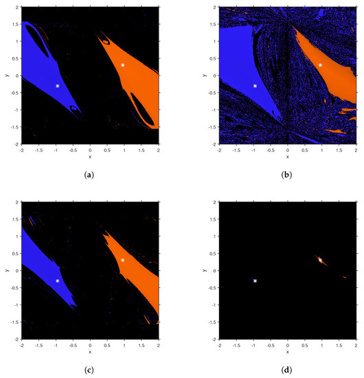
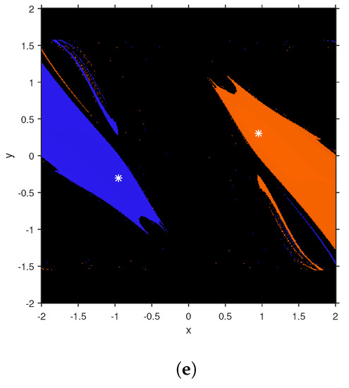
Figure 1. Basins of attraction of known and proposed methods on $F(x_1,x_2)=0$. (a) H${}_{6,1}$; (b) H${}_{6,2}$; (c) H${}_{6,3}$; (d) H${}_{6,4}$; (e) H${}_{9,1}$.

In Figure 1, the shape and wideness of the basins of attraction show that H${}_{6,1}$, H${}_{6,2}$, H${}_{6,3}$, and H${}_{6,4}$ can found any of both roots by using a great amount of initial estimations, some of them far from the roots. However, H${}_{6,4}$ is hardly able to find the roots and their basins are very small.

4.5. Example 5

Let us consider the nonlinear two-dimensional system $G(x_1,x_2)=0$ with coordinate functions

$$\begin{array}{ccc}\hfill g_1(x_1,x_2)& =& x_1^2+x_2^2-1,\hfill \end{array}$$

(41)

$$\begin{array}{ccc}\hfill g_2(x_1,x_2)& =& x_1^2-x_2^2+\frac{1}{2}.\hfill \end{array}$$

(42)

This system has four real solutions at points ${\left({\displaystyle \frac{1}{2}},{\displaystyle \frac{\sqrt{3}}{2}}\right)}^T$, ${\left({\displaystyle \frac{1}{2}},-{\displaystyle \frac{\sqrt{3}}{2}}\right)}^T$, ${\left(-{\displaystyle \frac{1}{2}},{\displaystyle \frac{\sqrt{3}}{2}}\right)}^T$, and ${\left(-{\displaystyle \frac{1}{2}},-{\displaystyle \frac{\sqrt{3}}{2}}\right)}^T$. Let us remark that they are symmetric as the system shows the intersection between two conical curves, an ellipse and a circumference. By using $x^{(0)}={(1,1)}^T$ as initial estimation, we have obtained the results appearing in Table 5, in which the residuals $\parallel x^{(k+1)}-x^{(k)}\parallel$ and $\parallel F(x^{(k+1)})\parallel$ also appear, for the three first iterations.

Table 5. Numerical results for Example 5.

	H${}_{6,1}$	H${}_{6,2}$	H${}_{6,3}$	H${}_{6,4}$	H${}_{9,1}$
$\parallel x^{(1)}-x^{(0)}\parallel$	$5.10\times {10}^{-1}$	$5.15\times {10}^{-1}$	$5.125\times {10}^{-1}$	$5.10\times {10}^{-1}$	$5.16\times {10}^{-1}$
$\parallel x^{(2)}-x^{(1)}\parallel$	$7.96\times {10}^{-3}$	$2.38\times {10}^{-3}$	$5.63\times {10}^{-3}$	$8.30\times {10}^{-3}$	$1.46\times {10}^{-3}$
$\parallel x^{(3)}-x^{(2)}\parallel$	$6.03\times {10}^{-12}$	$3.54\times {10}^{-16}$	$3.60\times {10}^{-13}$	$8.89\times {10}^{-12}$	$1.14\times {10}^{-23}$
$\parallel F(x^{(1)})\parallel$	$1.13\times {10}^{-2}$	$3.37\times {10}^{-3}$	$8.00\times {10}^{-3}$	$1.18\times {10}^{-2}$	$2.07\times {10}^{-3}$
$\parallel F(x^{(2)})\parallel$	$8.53\times {10}^{-12}$	$5.00\times {10}^{-16}$	$5.10\times {10}^{-13}$	$1.26\times {10}^{-11}$	$1.61\times {10}^{-23}$
$\parallel F(x^{(3)})\parallel$	$2.56\times {10}^{-56}$	$8.87\times {10}^{-62}$	$8.99\times {10}^{-57}$	$5.02\times {10}^{-54}$	$6.87\times {10}^{-161}$

The numerical results appearing in Table 5 show as the estimation of the roots has similar errors in all sixth order methods, although H${}_{6,2}$ and H${}_{6,3}$ are slightly better than H${}_{6,1}$. Indeed, the ninth order scheme has the best precision in the approximation of the roots of $G(x_1,x_2)$, as corresponds to its high order of convergence. In terms of computational time, the mean of one hundred consecutive iterations have been used in order to get good estimations of the real time and, in case of proposed methods, they use similar times as the existing schemes getting better accuracy.

In Figure 2 the colors blue, orange, green and purple correspond to the basins of the roots of the system (41). We can see the dynamical planes of the proposed method methods H${}_{6,1}$ and H${}_{9,1}$ and known schemes H${}_{6,2}$, H${}_{6,3}$, and H${}_{6,4}$ when they are applied on system $G(x_1,x_2)=0$.

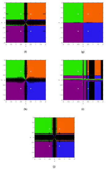
Figure 2. Basins of attraction of known and proposed methods on $G(x_1,x_2)=0$. (a) H${}_{6,1}$; (b) H${}_{6,2}$; (c) H${}_{6,3}$; (d) H${}_{6,4}$; (e) H${}_{9,1}$.

Regarding the stability of proposed and known iterative processes on $G(x_1,x_2)$, it can be observed in Figure 2 that, in all cases except H${}_{6,4}$, the connected component of the basins of attraction that holds the root (usually known as immediate basin of attraction) is very wide. For all iterative methods black areas of low convergence or divergence appear, being more diffuse in case of H${}_{6,2}$ and wider in H${}_{6,4}$. Methods H${}_{6,1}$, H${}_{6,3}$ and H${}_{9,1}$ present black areas that are mainly regions of slower convergence, that would be colored if a higher number of iterations is fixed as a maximum; meanwhile, the biggest black area of the dynamical plane associated to method H${}_{6,4}$ corresponds to divergence.

5. Concluding Remarks

From Potra–Pták third order scheme, an efficient sixth order method for solving nonlinear system is proposed. Moreover, it has been extended by adding subsequent steps with the same structure that adds a new functional evaluation per new step. Then the order of the resulting procedure increases in three units per step. The proposed methods have been shown to be more efficient that several known methods of the same order. Some numerical tests with academic and real-life problems have been made to check the efficiency and applicability of the designed procedures. The numerical performance have been opposed to the stability shown by the dynamical planes of new and known methods on two-dimensional systems.

References

- Ostrowski, A.M. Solution of Equations and Systems of Equations; Academic Press: New York, NY, USA, 1966. [Google Scholar]
- Ortega, J.M.; Rheinboldt, W.C. Iterative Solution of Nonlinear Equations in Several Variables; Academic Press: New York, NY, USA, 1970. [Google Scholar]
- Kelley, C.T. Solving Nonlinear Equations with Newton’s Method; SIAM: Philadelphia, PA, USA, 2003. [Google Scholar]
- Traub, J.F. Iterative Methods for the Solution of Equations; Prentice-Hall: Englewood Cliffs, NJ, USA, 1964. [Google Scholar]
- Homeier, H.H.H. A modified Newton method with cubic convergence: The multivariable case. J. Comput. Appl. Math. 2004, 169, 161–169. [Google Scholar] [CrossRef]
- Darvishi, M.T.; Barati, A. A fourth-order method from quadrature formulae to solve systems of nonlinear equations. Appl. Math. Comput. 2007, 188, 257–261. [Google Scholar] [CrossRef]
- Cordero, A.; Hueso, J.L.; Martínez, E.; Torregrosa, J.R. A modified Newton-Jarratt’s composition. Numer. Algor. 2010, 55, 87–99. [Google Scholar] [CrossRef]
- Cordero, A.; Hueso, J.L.; Martínez, E.; Torregrosa, J.R. Efficient high-order methods based on golden ratio for nonlinear systems. Appl. Math. Comput. 2011, 217, 4548–4556. [Google Scholar] [CrossRef]
- Grau-Sánchez, M.; Grau, À.; Noguera, M. On the computational efficiency index and some iterative methods for solving systems of nonlinear equations. J. Comput. Appl. Math. 2011, 236, 1259–1266. [Google Scholar] [CrossRef]
- Grau-Sánchez, M.; Grau, À.; Noguera, M. Ostrowski type methods for solving systems of nonlinear equations. Appl. Math. Comput. 2011, 218, 2377–2385. [Google Scholar] [CrossRef]
- Potra, F.-A.; Pták, V. Nondiscrete Induction and Iterarive Processes; Pitman Publishing: Boston, MA, USA, 1984. [Google Scholar]
- Grau-Sánchez, M.; Noguera, M.; Amat, S. On the approximation of derivatives using divided difference operators preserving the local convergence order of iterative methods. J. Comput. Appl. Math. 2013, 237, 363–372. [Google Scholar] [CrossRef]
- Sharma, J.R.; Arora, H. On efficient weighted-Newton methods for solving systems of nonlinear equations. Appl. Math. Comput. 2013, 222, 497–506. [Google Scholar] [CrossRef]
- Cordero, A.; Torregrosa, J.R. Variants of Newton’s method using fifth order quadrature formulas. Appl. Math. Comput. 2007, 190, 686–698. [Google Scholar] [CrossRef]
- Chicharro, F.I.; Cordero, A.; Torregrosa, J.R. Drawing dynamical and parameter planes of iterative families and methods. Sci. World J. 2013, 2013, 780153. [Google Scholar] [CrossRef] [PubMed]
© 2018 by the authors. Licensee MDPI, Basel, Switzerland. This article is an open access article distributed under the terms and conditions of the Creative Commons Attribution (CC BY) license (http://creativecommons.org/licenses/by/4.0/).