Abstract
A new algorithm is proposed for polynomial or rational approximation of the planar offset curve. The best rational Chebyshev approximation could be regarded as a kind of geometric approximation along the fixed direction. Based on this idea, we developed a wholly new offset approximation method by changing the fixed direction to the normal directions. The error vectors follow the direction of normal, and thus could reflect the approximate performance more properly. The approximation is completely independent of the original curve parameterization, and thus could ensure the stability of the approximation result. Experimental results show that the proposed algorithm is reasonable and effective.
1. Introduction
Offset curves are widely used in various computer-aided design and manufacturing (CAD/CAM) areas, such as tool path generation [1,2], 3D numerical control (NC) machining [3,4], solid modeling [5], graphics [6], and so on. However, the offset curve usually cannot be represented in a polynomial or rational form, and thus is difficult to apply in CAD systems.
Many methods for the offset approximation have been proposed and developed. Cobb [7] proposed a new control net by translating each control point, whereas Tiller and Hanson [8] developed the idea by translating each edge of the control polygon. Hoschek [9] suggested a least squares solution, Piegl and Tiller [10] employed sample interpolation, and Cheng and Wang [11] used Jacobi series to approximate the offset curve. Lee et al. [12] regarded the offset curve as a convolution of a sweeping circle, Ahn et al. [13] used conic approximation to approximate the sweeping circle, and Zhao and Wang [14] employed second-order rational polynomials, and achieved high-precision approximation.
Some algorithms, such as those proposed by Piegl and Tiller [10] and Lee et al. [12], employ the point-sample technique for fast and convenient calculation. However, when the input curve changes its parameterization, the algorithms will take it as a new curve, and generate a wholly different approximation result.
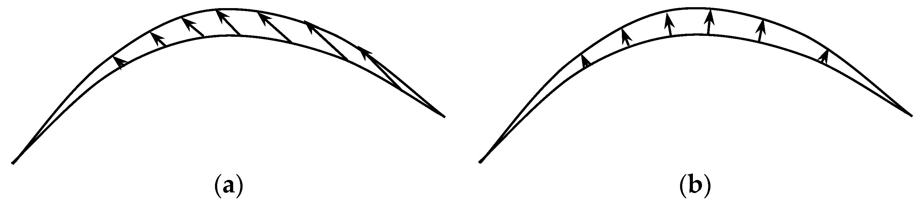
When the error calculation depends on curve parameterization, there will also be problems. Suppose the original curve, the offset curve, and the approximation curve are represented by , , and , respectively. The offset radius is . There are two error calculation formulas: and [15]. However, they sometimes are not able to accurately estimate the real approximating error. Figure 1 shows two kinds of point correspondence between the original curve and its approximation. Although the approximation curve is the same, the above error calculation formulas produce different results.
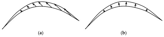
Figure 1.
Two methods of point correspondence. (a) Approximation in a specified direction; (b) Approximation in the normal direction.
In this paper, a new offset approximation method is proposed, which approximates the offset curve directly in the normal direction. The distance error in normal directions is more suitable to evaluate the approximation precision, which is independent of the parameterization, and fits closely with human perception. Whatever parameterization the input curve uses, the approximation curve and the error estimation always remain the same. Using the idea of the best rational Chebyshev approximation for reference, the new method generates rational approximation to the planar offset curve. The paper is organized as follows. Section 2 briefly reviews the basic theory of the best rational Chebyshev approximation. Section 3 introduces our offset approximation method. Section 4 gives some experiments. Finally, Section 5 concludes the paper.
2. Best Rational Chebyshev Approximation Theory
Consider a set of polynomials and rational polynomials:
where . When , it comes a k-degree polynomial.
The rational function is called the best Chebyshev rational approximation of the given continuous function , when the choice of values of and minimizes the maximum absolute value , where [16].
Theorem.
If is continuous, there is a unique choice of the values of and that minimizes . For this choice, has extrema in , all of magnitude and with alternating signs.
Suppose is the extremum of the minimax solution, then the satisfied equations will be:
where alternates for the alternating extrema. Besides and in the equation, is an additional unknown.
It is difficult to find the coefficients and maximum deviation in the set of equations listed in (1), which is highly nonlinear in . Remes [16] suggested an iterative method to find the approximation. Press et al. [17] proposed a speed-up algorithm, which solves linear equations at each step, and can greatly reduce the computation complexity.
3. Rational Offset Approximation along the Normal Direction
Suppose is a regular rational Bézier curve with the degree of , and is its unit normal vector. The offset curve with radius can be represented by . In the following, a polynomial
or a rational curve
is to be found to approximate the offset curve along the normal direction, where .
The abscissa and ordinate of the offset curve could be approximated respectively to obtain rational approximate functions. However, we have to find a common denominator to obtain a rational Bézier curve. The operation may increase the function degree and produce a second-order error.
Inspired by the best rational Chebyshev approximation theory, a wholly new approximation method is proposed. All error vectors of the best Chebyshev rational approximation are parallel to the Y-axis. By changing the direction of the error vectors to the normal direction, a high-precision approximation method is obtained. The approximation curve is assumed to intersect the offset curve at several locations. Then, the domain is subdivided into subintervals. Suppose the error extrema are equal in each subinterval, and set up a set of equations to calculate the approximation. This idea will be introduced in detail as follows, taking the rational approximation as an example.
The error is measured as the distance between the two parameter points and , which are located on the same normal curve , so it could be represented as , where the sign denotes the dot product. Let denote the maximum absolute value of . Suppose there are parameters, , which satisfy
that is,
where the sign alternates for the alternating extrema.
The above vector equations can be split into the following two kinds of equations, one for the direction, and the other for the magnitude:
where the sign denotes the cross product. For the first part of Equation (2), the 2D vectors can be regarded as 3D vectors by defining the coordinate , and the system of Equation (2) could be represented by the following matrices:
where , , and are two square matrices of order , and and are two column vectors of order . Let and respectively denote the th column vector of and , and and respectively denote the th element of and , where . There are:
In Equation (2), there are equations and unknown quantities, including coefficients of and the extremum . Therefore, the number of extrema could be or to obtain consistent equations, when the degree is even or odd, respectively.
Equation (2) is highly nonlinear since is additionally unknown. It can be solved efficiently by an iterative method. The main steps are as follows:
- (i).
- Initialize the extrema ;
- (ii).
- Solve Equation (2) and obtain the coefficients and as well as the extremum ;
- (iii).
- Compute the actual error extrema for ;
- (iv).
- Replace the value with the nearest actual extremum of the same sign;
- (v).
- Go back to step (ii) and iterate to convergence.
Exact extrema may be not so important as the approximation curve is the wanted solution, so we could dispense with keeping track of the actual extrema. The approximation error could be measured at the given parameter points. An accelerated algorithm is proposed as follows:
- (i).
- Set the values of , and the extremum ;
- (ii).
- Solve Equation (2) and obtain the coefficients and ;
- (iii).
- Compute the actual error at , and the sign ;
- (iv).
- Replace the extremum with the average error, and replace the approximation curve value at with ;
- (v).
- Go back to step (ii) and iterate to convergence.
The initial values of are set following the method used in the program proposed in Press et al. [17]. A polynomial could be regarded as a degenerate rational case whose denominator is 1. Thus, the polynomial approximation curve could also be obtained by the above algorithm when the coefficients are set in the first step.
4. Experiments
Some experiments are given to show the reasonableness and effectiveness of our algorithm.
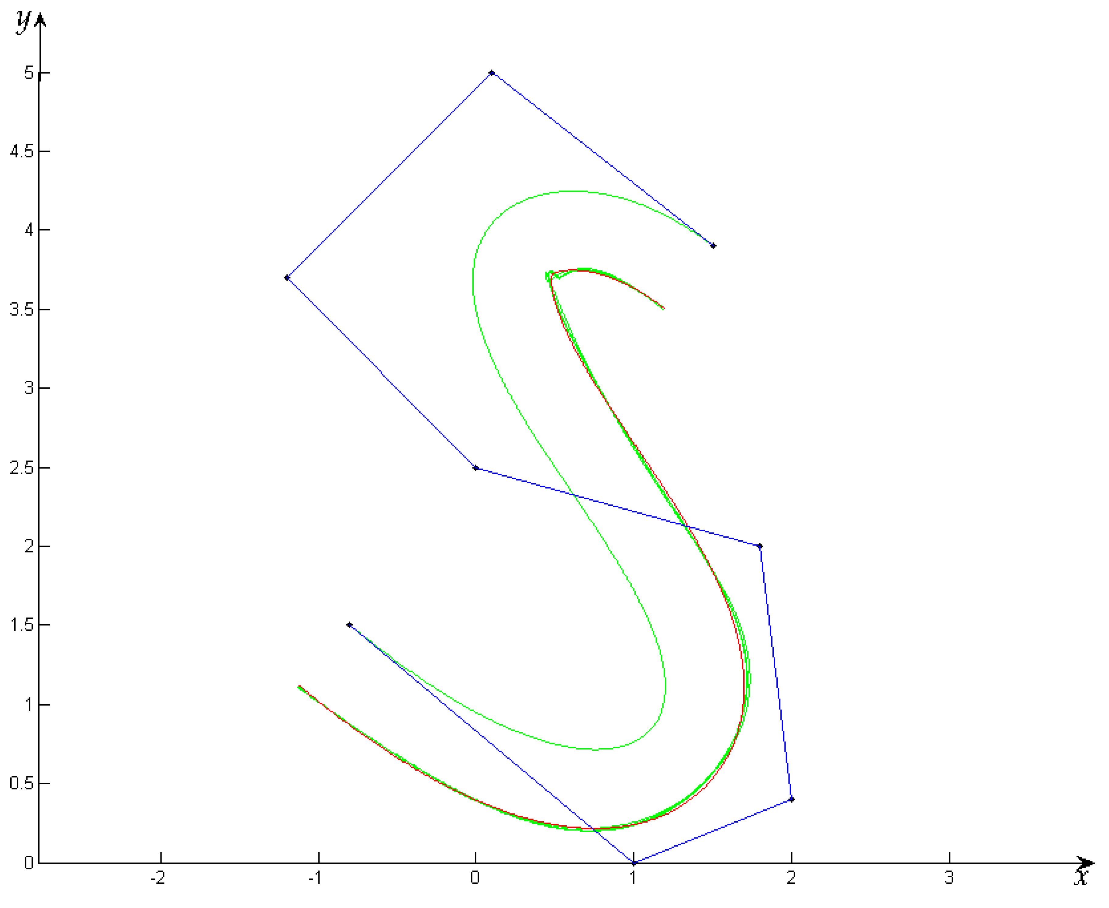
A septic Bézier curve is shown in Figure 2. The control points are (−0.8, 1.5), (1, 0), (2, 0.4), (1.8, 2), (0, 2.5), (−1.2, 3.7), (0, 1.5), (1.5, 3.9), and the radius is 0.5. Taking the curve as an example, we will verify the effectiveness of our approximation algorithm in terms of the approximation direction and precision.
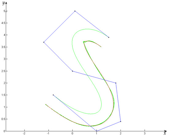
Figure 2.
The septic Bézier curve and the offset. The original curve is the thin green curve with a control net. The offset is the red curve, and the approximating offset is the thick green curve.
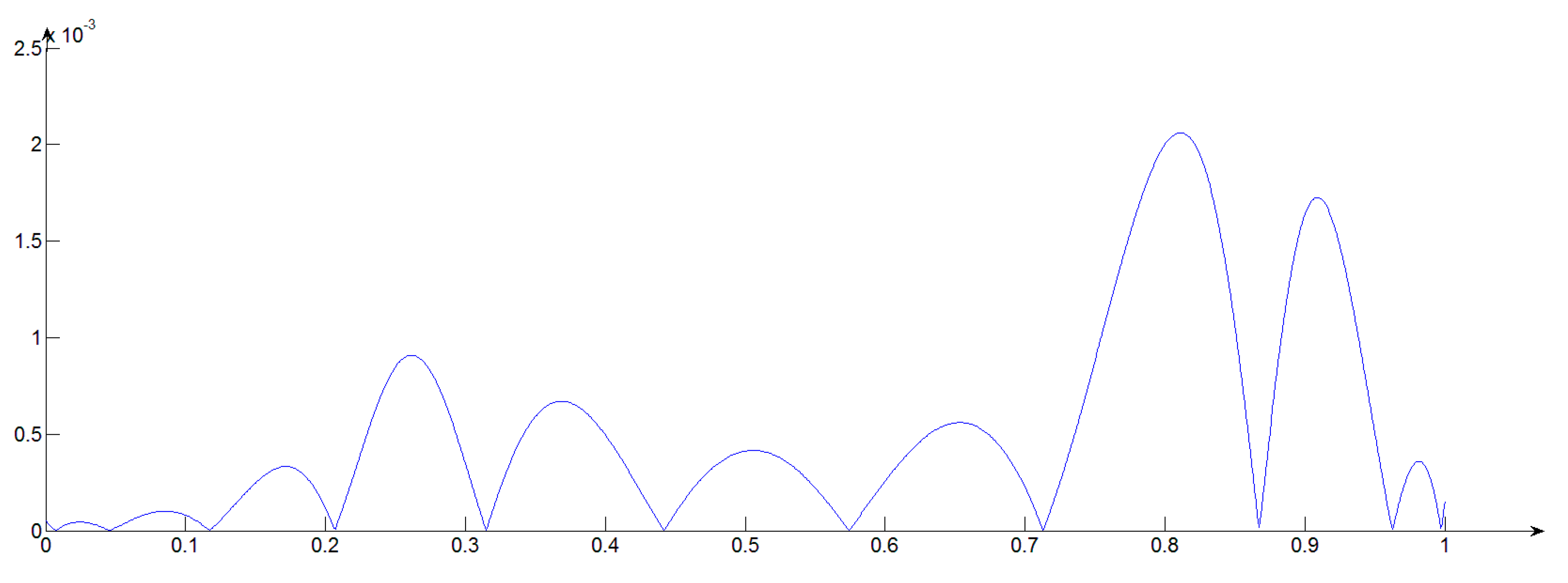
In the following, the position relationship of parameter points between the offset and its approximating curve are investigated. The two corresponding curve points should be located on the same normal curve. That is, the direction of the error vector should be parallel to that of the normal vector N(t). Here, the length of the vector represented by is calculated. Considering the unavoidable calculation error, the result should fluctuate around zero. Figure 3 shows the fluctuation curve of the approximation curve obtained by our accelerating iterative algorithm. The curve is the result obtained after the second iteration. Apparently, the curve values are nearly equal to zero, which sufficiently proves that the proposed algorithm approximates the offset curve along the normal direction.
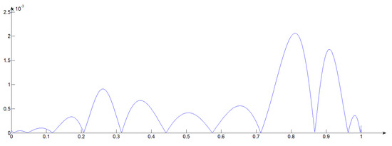
Figure 3.
Fluctuation curve of the direction deviation.
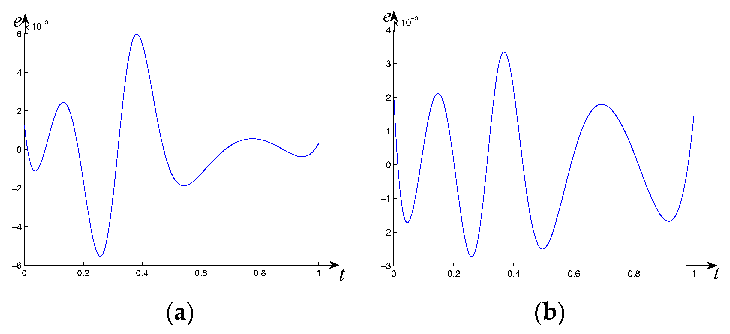
The interpolating method could not guarantee the approximation error, but it is rather convenient in application. When the sample points are carefully selected, the precision is enhanced. However, a number of the sample points may increase greatly when the curve becomes slightly more complex. Our method is rarely influenced by the change of the curve during the theoretical support. For example, the number of the sample points is less than when running the accelerated iterative method. A comparison between the error bounds obtained by the interpolating method and our accelerating method is given as follows. Using 500 sample points, the error bound generated by the interpolating method is 0.0371 (see Figure 4a). Using 96 sample points, the error bound of our algorithm is 0.0428 for the first iteration, and 0.0363 after the second iteration (see Figure 4b).
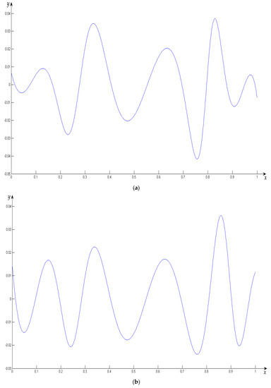
Figure 4.
Error curves of different approximation methods. (a) Interpolating algorithm; (b) Algorithm in this paper after the second iteration.
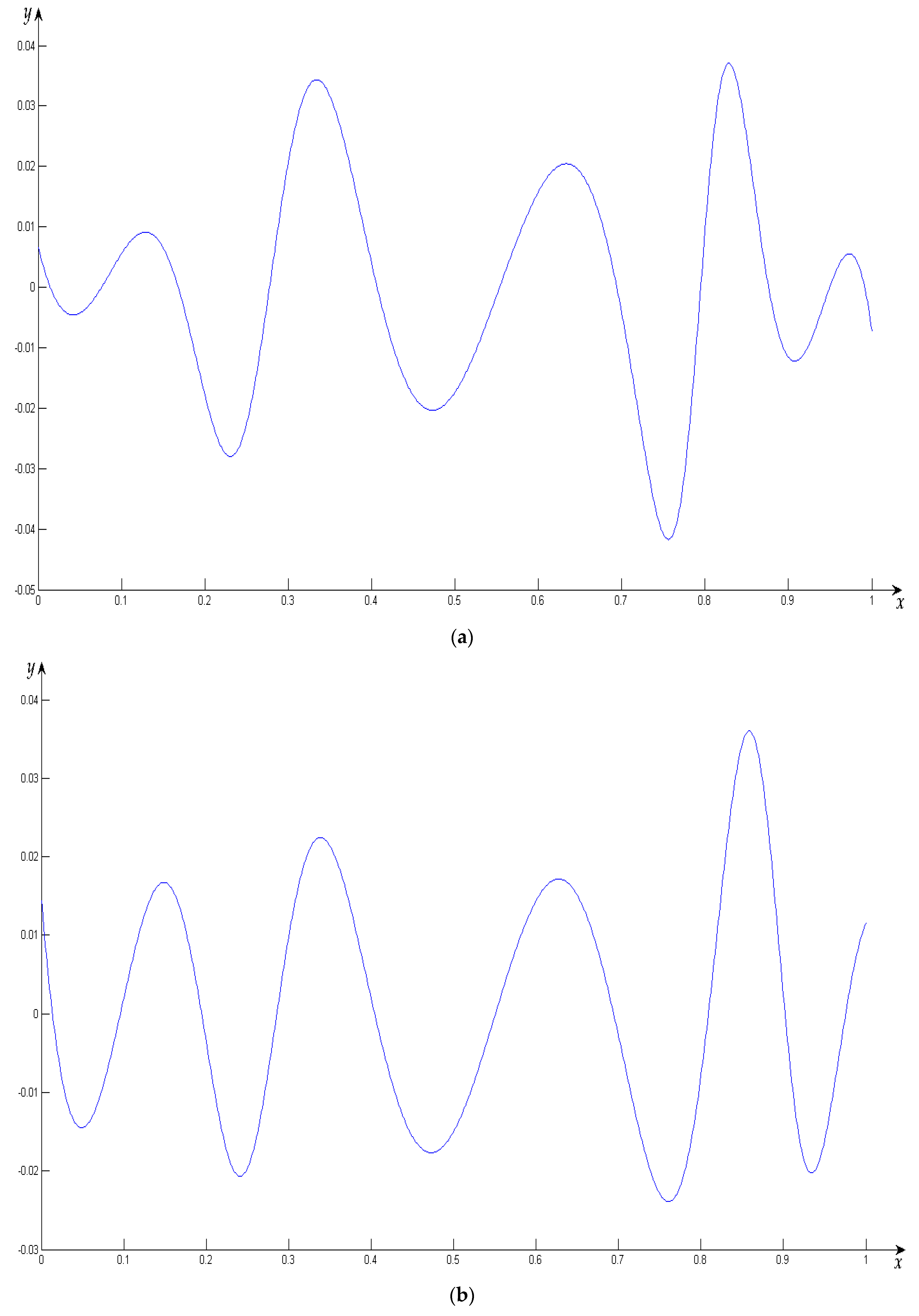
Lee’s method [12] is regarded as classical in offset approximation, which is simple and highly precise. Ahn et al. made an improvement of their work to reduce the degree of the approximation curve [13]. A comparison is made between our method and their work in terms of the precision in the following. Figure 5 is a quintic Bézier curve with six control points (3, −1), (4, 2), (4.5, 2), (5.5, 1.5), (6.5, 0), and (7, −1). Figure 5 shows the approximation error performance. Table 1 shows the error distance along the norm direction of each method. Lee’s method generates a rational approximation curve with degree 21. Ahn’s method yields a polynomial curve with the same degree. Our method can approximate the offset with an arbitrary degree, and a quintic rational approximation is given for comparison. It can be seen that our error bound is better than Lee’s and Ahn’s error estimation. The advantage is more obvious after the curve is subdivided, and the results are shown in the third and the fourth rows of Table 1.
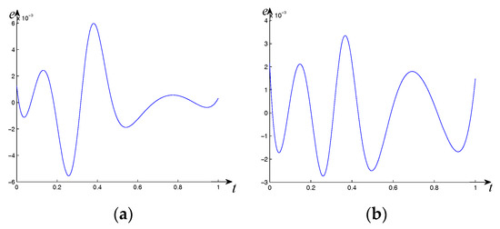
Figure 5.
Approximation error performance. (a) After the first iteration; (b) After four iterations.

Table 1.
Comparison between Lee’s, Ahn’s, and our algorithms in terms of the error bound.
5. Conclusions
This paper developed a method of polynomial and rational approximation for planar curves. The traditional recognition of the best rational Chebyshev approximation is presented. The approximation direction is investigated, and the algebraic method could be regarded as a geometric approximation method. By changing the approximation direction from the Y-axis to the normal direction, a high-precision approximation is developed. The method is driven by geometric constraints, so the approximation process is independent of parameterization. The directions of the error vectors are along the normal direction, so the error estimation fits closely with human perception. The experiments show the reasonableness and the effectiveness of the proposed algorithm. The method could be used in the approximation of complex curves or surfaces, and applied in the area of interval curves.
Acknowledgments
This work was supported by the National Natural Science Foundation of China (No. 61402281, 11401373) and the Natural Science Foundation of Shanghai 16ZR1413700.
Author Contributions
Hongyan Zhao and Lian Zhou conceived and designed the experiments; Hongyan Zhao performed the experiments; Lian Zhou analyzed the data; Lian Zhao contributed reagents/materials/analysis tools; Hongyan Zhao wrote the paper.
Conflicts of Interest
The authors declare no conflict of interest.
References
- Hansen, A.; Arbab, F. An algorithm for generating NC tool paths for arbitrarily shaped pockets with islands. ACM Trans. Graph. 1992, 11, 152–182. [Google Scholar] [CrossRef]
- Lasemi, A.; Xue, D.; Gu, P. Recent development in CNC machining of freeform surfaces: A state-of-the-art review. Comput. Aided Design 2010, 42, 641–654. [Google Scholar] [CrossRef]
- Chen, Y.; Ravani, B. Offset surface generation and contouring in computer-aided design. J. Mech. Transm. and Automation 1987, 109, 133–142. [Google Scholar] [CrossRef]
- Xu, C.; Zhang, S.; Huang, B.; Li, X.; Huang, R. NC process reuse oriented effective subpart retrieval approach of 3D CAD models. Comput. Ind. 2017, 90, 1–16. [Google Scholar] [CrossRef]
- Lynn, R.; Contis, D.; Hossain, M.; Huang, N.; Tucker, T.; Kurfess, T. Voxel model surface offsetting for computer-aided manufacturing using virtualized high-performance computing. J. Manuf. Syst. 2017, 43, 296–304. [Google Scholar] [CrossRef]
- Zhu, X.; Jin, X.; You, L. High-quality tree structures modelling using local convolution surface approximation. Vis. Comput. 2015, 31, 69–82. [Google Scholar] [CrossRef]
- Cobb, E. Design of Sculptured Surfaces Using the B-Spline Representation. Ph.D. Thesis, University of Utah, Salt Lake City, UT, USA, 1984. [Google Scholar]
- Tiller, W.; Hanson, E. Offsets of two-dimensional profiles. IEEE Comput. Graph. Appl. 1984, 4, 36–46. [Google Scholar] [CrossRef]
- Hoscheck, J. Spline approximation of offset curves. Comput. Aided Geom. Design 1988, 20, 33–40. [Google Scholar] [CrossRef]
- Piegl, L.; Tiller, W. Computing offsets of NURBS curves and surfaces. Comput. Aided Design 1999, 31, 147–156. [Google Scholar] [CrossRef]
- Cheng, M.; Wang, G. Rational offset approximation of rational Bézier curves. J. Zhejiang Univ. 2006, 7, 1561–1565. [Google Scholar] [CrossRef]
- Lee, I.; Kim, M.; Elber, G. Planar curve offset based on circle approximation. Comput. Aided Design 1996, 28, 617–630. [Google Scholar] [CrossRef]
- Ahn, Y.; Kim, Y.; Shin, Y. Approximation of circular arcs and offset curves by Bézier curves of high degree. J. Comput. Appl. Math. 2004, 167, 405–416. [Google Scholar] [CrossRef]
- Zhao, H.; Wang, G. Offset approximation based on reparameterizing the path of a moving point along the base circle. Appl. Math. J. Chin. Univ. 2009, 24, 431–442. [Google Scholar] [CrossRef]
- Elber, G.; Lee, I.; Kim, M. Comparing offset curve approximation methods. IEEE Comput. Graph. Appl. 1997, 17, 62–71. [Google Scholar] [CrossRef]
- Ralston, A. Rational Chebyshev approximation by Remes’ algorithms. Numer. Math. 1965, 7, 322–330. [Google Scholar] [CrossRef]
- Press, W.; Teukolsky, S.; Vetterling, W.; Flannery, B. Numerical Recipes: The Art of Scientific Computing, 3rd ed.; Cambridge University Press: Cambridge, UK, 2007; pp. 247–250. [Google Scholar]
© 2017 by the authors. Licensee MDPI, Basel, Switzerland. This article is an open access article distributed under the terms and conditions of the Creative Commons Attribution (CC BY) license (http://creativecommons.org/licenses/by/4.0/).