A Normal and Standard Form Analysis of the JWKB Asymptotic Matching Rule via the First Order Bessel’s Equation

Abstract

Traditional first order JWKB method ($=:{\left(JWKB\right)}_1$) is a conventional semiclassical approximation method mainly used in quantum mechanical systems for accurate solutions. ${\left(JWKB\right)}_1$ general solution of the Time Independent Schrodinger’s Equation (TISE) involves application of the conventional asymptotic matching rules to give the accurate wavefunction in the Classically Inaccessible Region (CIR) of the related quantum mechanical system. In this work, Bessel Differential Equation of the first order ($=:{\left(BDE\right)}_1$) is chosen as a mathematical model and its ${\left(JWKB\right)}_1$ solution is obtained by first transforming into the normal form via the change of independent variable. The ${\left(JWKB\right)}_1$ general solution for appropriately chosen initial values in both normal and standard form representations is analyzed via the generalized ${\left(JWKB\right)}_1$ asymptotic matching rules regarding the ${\tilde{S}}_{ij}$ matrix elements given in the literature. Instead of applying the common ${\left(JWKB\right)}_1$ asymptotic matching rules relying on the physical nature of the quantum mechanical system, i.e., a physically acceptable (normalizable) wavefunction, a pure semiclassical analysis is studied via the ${\left(BDE\right)}_1$ model mathematically. Finally, an application to a specific case of the exponential potential decorated quantum mechanical bound state problem is presented.

1. Introduction

The ${\left(JWKB\right)}_1$ method (we simply refer to the “n-th order JWKB (or WKB)” by a simple abbreviation: ${\left(JWKB\right)}_n$) is conventionally known to be a strong and effective semiclassical approximation method enabling accurate analytical solutions in quantum mechanical systems, i.e., [1,2,3,4,5,6,7,8,9,10]. Quantum mechanical systems described by the Time Independent Schrodinger’s Equation (TISE), which is in the form of a linear second order homogenous (normal form) differential equation:

$$y^{″}\left(x\right)+f\left(x\right)y\left(x\right)=0,$$

(1a)

$$f\left(x\right)=k^2\left(x\right)=\frac{2m}{{\hslash }^2}\left[E-V\left(x\right)\right]$$

(1b)

where these terms have their usual meanings (m represents mass; ℏ represents Planck’s constant divided by $2\pi$; E represents total energy; and $V\left(x\right)$ represents the potential function), have exact and approximate ${\left(JWKB\right)}_1$ solutions in the following forms:

$$y_{EX}\left(x\right)=:y\left(x\right)=k_1{y}_1\left(x\right)+k_2{y}_2\left(x\right),$$

(2a)

$$y_{JWKB}\left(x\right)=:\tilde{y}\left(x\right)={\tilde{k}}_1{\tilde{y}}_1\left(x\right)+{\tilde{k}}_2{\tilde{y}}_2\left(x\right),$$

(2b)

where $k_1\&k_2$ and ${\tilde{k}}_1\&{\tilde{k}}_2$ are the arbitrary constants and, $y_1\&y_2$ and ${\tilde{y}}_1\&{\tilde{y}}_2$ are the exact and ${\left(JWKB\right)}_1$ complementary solutions, respectively. These constant coefficients in the exact and ${\left(JWKB\right)}_1$ general solutions can be found from given initial values. The ${\left(JWKB\right)}_1$ solution has a typical property that both complementary ${\left(JWKB\right)}_1$ solutions (and hence, the ${\left(JWKB\right)}_1$ general solution) diverge at a small region around the classical turning point where $f\left(x\right)=0\Rightarrow E=V\left(x\right)$, i.e., [3,4,5]. Moreover, the ${\left(JWKB\right)}_1$ general solution in (2b) can be accurate for the Classically Accessible Region (CAR) under some circumstances, but always needs asymptotic matching in the Classically Inaccessible Region (CIR) for accurate ${\left(JWKB\right)}_1$ solutions [3,4]. CAR is the classically accessible region where the particle can classically exist since its potential energy is smaller than its total energy: $f\left(x\right)>0\Rightarrow E>V\left(x\right)$; and CIR is the classically inaccessible region where it cannot classically exist since its potential energy is greater than its total energy: $f\left(x\right)<0\Rightarrow E<V\left(x\right)$. Conventional ${\left(JWKB\right)}_1$ asymptotic matching rules require either of the complementary solutions in (2b) to be canceled in the CIR as follows [3,4]:

$${\tilde{y}}^{m.}\left(x\right)=\left\{\begin{array}{c}\tilde{y}\left(x\right)\mathrm{for}\mathrm{CAR}:f\left(x\right)>0\hfill \\ \mathrm{either}{\tilde{k}}_1{\tilde{y}}_1\left(x\right)\mathrm{or}{\tilde{k}}_2{\tilde{y}}_2\left(x\right)\mathrm{for}\mathrm{CIR}:f\left(x\right)<0\hfill \end{array}\right.,$$

(3)

and the resultant asymptotically-matched solution should assure:

$${\tilde{y}}^{m.}\left(x\right)\to \left\{\begin{array}{c}\underset{x\to -\infty }{lim}\tilde{y}\left(x\right)=0\mathrm{if}\mathrm{CIR}\mathrm{lies}\mathrm{on}\mathrm{the}\mathrm{LHS}\\ \underset{x\to \infty }{lim}\tilde{y}\left(x\right)=0\mathrm{if}\mathrm{CIR}\mathrm{lies}\mathrm{on}\mathrm{the}\mathrm{RHS}\end{array}\right.,$$

(4)

where ${\tilde{y}}^{m.}\left(x\right)$ represents the asymptotically-matched ${\left(JWKB\right)}_1$ general solution. In other words, the asymptotically diverging term in the CIR should be canceled in the general solution so that (4) can hold. The formal ${\left(JWKB\right)}_{N\to \infty }$ approximation formula involving both complementary functions in (2b) is actually in the form of an infinite series:

$${\tilde{y}}_{\infty }\left(x\right)=exp\left[\frac{1}{\delta }\sum _{n=0}^N{\delta }^n{S}_n\left(x\right)\right],\left(\begin{array}{c}\delta \to 0\\ N\to \infty \end{array}\right),$$

(5)

where $\delta =\hslash /i\to 0$ for the TISE and $S_n$ represents the expansion terms given in [3,4], and the two-valuedness of these expansion terms gives two complementary ${\left(JWKB\right)}_N$ functions. However, only the first two terms (with indices $i=0$ and 1) are used in the ${\left(JWKB\right)}_1$ approximation. Moreover, ${\left(JWKB\right)}_1$ gives accurate-enough solutions for slowly-changing potentials in the TISE, and a criterion for this is given as follows [3,4,5]:

$$0\le g\left(x\right)=\left|\frac{{\partial }_{xx}k\left(x\right)}{2k^3\left(x\right)}-\frac{3{\left[{\partial }_{x}k\left(x\right)\right]}^2}{4k^4\left(x\right)}\right|<<1.$$

(6)

As the potential in the TISE in (1b) gets sharper, (6) fails, and some of the higher order terms can no longer be neglected; and the higher order JWKB approximation (= ${\left(JWKB\right)}_{N>1}$) is required for accurate-enough solutions [1,2,3,4,5,6,7]. Therefore, for a general potential $V\left(x\right)$ involving both smooth and sharp sub-domains in the corresponding normal form (the TISE), say $S{D}_1$ (for the smooth) and $S{D}_2$ (for the sharp), respectively, the ${\left(JWKB\right)}_1$ approximation always gives accurate general solution in $S{D}_1\in CAR$ and inaccurate (but asymptotically matchable) solutions in $S{D}_1\in CIR$; however, ${\left(JWKB\right)}_{N>1}$ is required for $S{D}_2\in CAR\cup S{D}_2\in CIR$ [3,4,5]. Such a potential with obedient (smooth potential = $S{D}_1$) and non-obedient (sharp potential = $S{D}_2$) subdomains in the corresponding TISE is studied semiclassically by the first order Bessel Differential Equation, ${\left(BDE\right)}_1$, as a chosen model differential equation here. Our aim here is to show these physical results by a successful semiclassical analysis mathematically only (not physically).

Since the ${\left(JWKB\right)}_1$ method is generally applied to the quantum mechanical systems, the main principles of the existing asymptotic matching rules rely on the nature of the physical system under study, i.e., a physically-acceptable bound state wave function (solution of the TISE) in the CIR should not asymptotically diverge to infinity (which means Equation (4)) so that it can be normalized in $x\in (-\infty ,\infty )$ [3,4,5]. This result is the physical consequence of the asymptotic matching rule in the $S{D}_1\in CIR$ for the ${\left(JWKB\right)}_1$. Its semiclassical explanation for the Simple Linear Potential (SLP), as a model potential where the ${\left(JWKB\right)}_1$ applicability criterion is satisfied in the entire domain, was studied in terms of the ${\left(JWKB\right)}_N$ expansion terms in [4]. In this work, similarly, a pure semiclassical analysis of the asymptotic matching rules is studied for the intentionally-chosen ${\left(BDE\right)}_1$ where the ${\left(JWKB\right)}_1$ applicability criterion is now partially satisfied in some subdomains involving both CAR and CIR. In other words, $S{D}_1$ and $S{D}_2$ coexist in the whole domain of our ${\left(BDE\right)}_1$ with a successive turning point so that $CAR$ and $CIR$ are guaranteed. In our analysis, appropriately-chosen associated initial values are used to compare the general asymptotically-unmatched and -matched ${\left(JWKB\right)}_1$ solutions with the related exact general solutions. ${\left(JWKB\right)}_1$ solutions of some quantum mechanical systems involving exponential potential-decorated TISE, which is associated with the ${\left(BDE\right)}_n$, were studied by the use of the common asymptotic matching rules given in (4) in the literature [10,11,12]. Our aim here is rather to search the asymptotic modifications of the ${\left(JWKB\right)}_1$ approximation for the ${\left(BDE\right)}_1$ mathematically via the semiclassical theories where the physical nature of the system regarding the bound and unbound quantum mechanical system analysis is no longer interfered. We expect to find the same asymptotically-matched ${\left(JWKB\right)}_1$ wavefunction solution as in [10,11,12]. It is also shown here for a specific case of the exponential potential decorated TISE in Section 5.

The ${\left(BDE\right)}_1$ is given in the standard form by:

$$y^{″}+\frac{1}{x}{y}^{\prime }+\frac{(x^2-1)}{x^2}y=0,$$

(7)

whose exact general solution in (2a) is the linear combination of two kinds of first order Bessel functions, namely:

$$y_1\left(x\right)=J_1\left(x\right)\mathrm{and}{y}_2\left(x\right)=Y_1\left(x\right).$$

(8a)

Their expressions in terms of infinite series are given as follows [13,14]:

$$J_1\left(x\right)=\sum _{i=0}^{\infty }\frac{{(-1)}^i{(x/2)}^{1+2i}}{i!\Gamma (i+2)}=\sum _{i=0}^{\infty }\frac{{(-1)}^i{(x/2)}^{1+2i}}{i!(1+i)!},$$

(8b)

$$Y_1\left(x\right)=\underset{p\to 1}{lim}\frac{J_p\left(x\right)cos\left(p\pi \right)-J_{-p}\left(x\right)}{sin\left(p\pi \right)}.$$

(8c)

The ${\left(JWKB\right)}_1$ solution of the ${\left(BDE\right)}_1$ in (7) can similarly be written (when solved) as a linear combination of two complementary functions as given in (2b). However, to follow this procedure, one has to face with the problem arising from the fact that one cannot find the ${\left(JWKB\right)}_1$ general solution given in (2b) directly by the conventional methods since the ${\left(JWKB\right)}_1$ technique including the famous ${\left(JWKB\right)}_1$ connection formulas requires (rather than that in (7)) a Linear Differential Equation (LDE) in the normal form given in (1a). Therefore, we have to study it in the normal form with a suitable change of variable. Complementary ${\left(JWKB\right)}_1$ functions (solutions) in (2b) can then be easily found by using the famous ${\left(JWKB\right)}_1$ connection formulas given in [1,2,3,4,5]. Once the ${\left(JWKB\right)}_1$ solution of either region (CAR or CIR) is found, the other region can directly be determined via these connection formulas.

Therefore, our interest here can be summarized as follows: (i) to find the ${\left(JWKB\right)}_1$ general solution of the ${\left(BDE\right)}_1$ whose structure is given in (2b) by using some appropriate change of variable to transform into a normal form (which is not unique); (ii) to check its accuracy in the (sub)domains of the CAR and the CIR where the ${\left(JWKB\right)}_1$ applicability criterion in (6) holds; and (iii) to find ways to do the correct asymptotic matching in the necessary (sub)domains by semiclassical analyses mathematically only. Our analyses should also show that asymptotic matching is required only for $S{D}_1\in CIR$ as the physical requirement (normalizability of quantum mechanical wave functions, which is in a bound state form here).

The ${\left(JWKB\right)}_1$ general solution of the ${\left(BDE\right)}_1$ is obtained here after having been transformed into the normal form via change of the independent variable so that the conventional ${\left(JWKB\right)}_1$ connection formulas given in [1,2,3,4,5] can be used along with the associated initial values, which have been intentionally chosen in the CAR. Comparisons with the exact solutions are being achieved by applying these carefully-chosen common initial values. Since our asymptotic matching rule gives a criterion for a semiclassically (not physically) acceptable ${\left(JWKB\right)}_1$ solution, we have the following semiclassical outcomes: (i) why ${\left(JWKB\right)}_1$ solutions are accurate in some domains in the CAR ($S{D}_1\in CAR$) and why they give inaccurate results in some other domains in the CIR ($S{D}_1\in CIR$); (ii) which complementary function in the general solution in (2b) (and also in the corresponding transformed representation) should be canceled in order to give an accurate general solution as desired by a successful asymptotic matching. Therefore, it can be thought of as an alternative and more general semiclassical matching rule for the present conventional ${\left(JWKB\right)}_1$ theories.

In Section 2, we give the statement and re-statement of our analyses based on the initial value-aided comparison in both standard and normal form representations. ${\left(JWKB\right)}_1$ solutions of the ${\left(BDE\right)}_1$ and their asymptotic matching in the transformed representations (in the normal form) are studied in Section 3, and the same calculations for the re-transformed representations (in the standard form) are studied in Section 4. Our semiclassical asymptotic matching rule neither involving exact solutions nor reasoning about the physical (quantum mechanical) nature of the system should give the correct asymptotic matching in both representations. We use the exact solutions only to show the accuracy and reliability of our alternative pure semiclassical asymptotic matching rule given in Section 3.2 (by Proposition 2). In Section 5, a physical application of our semiclassical asymptotic matching rule for a specific case of the exponential potential decorated bound state problem is presented. Preliminary work regarding the part “Calculations in The Normal Form” of Section 3 was discussed in the 19th International Conference on Applied Mathematics (AMATH’14)-Istanbul where some 2D analyses are available in [15]. (Note that Equations: (40) and (41a)–(41b) here are in the corrected form when compared with the misprints in [15]).

2. Statement and Re-Statement of the Problem

2.1. Associated IVP and Statement of The Problem

The process being followed here can be stated by the following proposition:

Proposition 1.

Once the ${\left(JWKB\right)}_1$ general solution in the form of (2b) is obtained, one can test the accuracy (or exactness) of this solution by comparing it with the exact general solution by applying the following initial values:

$$y\left(d_1\right)=y\left(x\right){|}_{x=d_1}={\alpha }_1\left(c\right),y^{\prime }\left(d_1\right)=\frac{dy\left(x\right)}{dx}{|}_{x=d_1}={\beta }_1\left(c\right),$$

(9)

where $d_1$ is some real constant and c is some parameter in the domain D where the ${\left(JWKB\right)}_1$ method is suitable for ($d_1,c$)$\in D$.

For the common initial values in (9), the exact general solution in (2a) gives:

$$y(c,x)=k_1\left(c\right)J_1\left(x\right)+k_2\left(c\right)Y_1\left(x\right),$$

(10)

where $k_1\left(c\right),k_2\left(c\right)$ are the c dependent coefficients satisfying the initial values given in (9), and the ${\left(JWKB\right)}_1$ general solution in (2b) gives:

$$\tilde{y}(c,x)={\tilde{k}}_1\left(c\right){\tilde{y}}_1\left(x\right)+{\tilde{k}}_2\left(c\right){\tilde{y}}_2\left(x\right),$$

(11)

where similarly, ${\tilde{k}}_1\left(c\right),{\tilde{k}}_2\left(c\right)$ are the c dependent coefficients satisfying the same initial values in (9). Since the common initial values are defined in continuous (or discrete) spectra in the domain of parameter c, both exact and ${\left(JWKB\right)}_1$ general solutions span the whole domain with parameter c to enable a successful comparison in two variables according to our proposition (Proposition 1) just as in [4]. However, we have to apply an appropriate change of variable and study it in the normal form as explained above. Note that parameter c is used in continuous spectra here, but in the application of the bound state problem in Section 5, it is a turning point parameter involving total energy, which is discrete.

2.2. Change of the Independent Variable and Re-Statement of the Problem

Lemma 1.

Although ${\left(BDE\right)}_1$ given in (7) is not in the normal form given in (1a), a simple change of the variable in the independent variable:

$$x:(-\infty ,\infty )\to (0,\infty ),x\left(\rho \right)=e^{\frac{c-\rho }{2}}$$

(12)

transforms the ${\left(BDE\right)}_1$ in the standard form in (7) to the following desired normal form (just as in (1a)) in a new independent variable, ρ:

$$\frac{d^{2}y\left(\rho \right)}{d{\rho }^2}+\frac{e^{c-\rho }-1}{4}y\left(\rho \right)=0.$$

(17)

Proof. 

Our proof is based on the following neat theorem:

Theorem 1.

The change of variable:

$$\rho \left(x\right)=\int exp\left[-\int p(x)dx\right]dx,u\left(\rho \right)=y\left(x\right)$$

(14)

transforms the differential equation in the standard form with the independent variable x given by:

$$y^{″}\left(x\right)+p\left(x\right)y^{\prime }\left(x\right)+q\left(x\right)y\left(x\right)=0$$

(15)

into the normal form with the independent variable ρ as follows:

$$u^{″}\left(\rho \right)+{\left\{q\left(x\right)exp\left[2\int p(x)dx\right]\right\}}_{x=x\left(\rho \right)}u\left(\rho \right)=0.$$

(16)

Proof. 

Suppose we have a change of variable $\rho =f\left(x\right)$ with $u\left(\rho \right)=y\left(x\right)$, then the derivatives:

$$\frac{d}{dx}=\frac{d\rho }{dx}\frac{d}{d\rho }=f^{\prime }\frac{d}{d\rho };\frac{d^2}{d{x}^2}=f^{{}^{\prime }2}\frac{d^2}{d{\rho }^2}+f^{″}\frac{d}{d\rho }$$

in (15) gives:

$$f^{{}^{\prime }2}{u}^{″}+f^{″}{u}^{\prime }+p{f}^{\prime }{u}^{\prime }+qu=0.$$

In order to eliminate the $u^{\prime }$ term, f must satisfy:

$$f^{″}+p{f}^{\prime }=0,$$

which gives:

$$f^{\prime }=exp\left(-\int p(x)dx\right)\Rightarrow f=\int exp\left(-\int p(x)dx\right)dx.$$

Additionally, the differential equation for u is in the form:

$$u^{″}+\frac{q}{f^{\prime 2}}u=0,$$

which is equivalent with (16). ☐       

☐

Various change of variable applications to transform the ${\left(BDE\right)}_n$ (with $n\to 1$ here) into any of the normal forms, which is not unique, are available in the literature, i.e., [14,16,17]. However, change of the independent variable given in (12) is suggested and followed here.

The procedure regarding the comparison of the ${\left(JWKB\right)}_1$ general solution with the exact general solution of our Initial Value Problem (IVP) here can be achieved as follows: Equation (13) can be re-written with two variables, ρ and c, where ρ represents the changed coordinates (rather than x, as explained above), and c (without loss of generality) represents the classical turning point ${\rho }_t=c$ satisfying $f(c,\rho )=0$, so that:

$${\partial }_{\rho }^{2}y(c,\rho )+f(c,\rho )y(\rho ,c)=0,$$

(17a)

where:

$$f(c,\rho )=k^2(c,\rho )=\frac{e^{c-\rho }-1}{4},-\infty <\rho <\infty ,$$

(17b)

whose initial values via Proposition (1) can now be used in the form:

$$y(c,\rho ){|}_{\rho =d_2}={\alpha }_2\left(c\right);\frac{\partial y(c,\rho )}{\partial \rho }{|}_{\rho =d_2}={\beta }_2\left(c\right).$$

(18)

Note that our notation here is as follows: we show the initial values in the original (standard form) system (in x) by subscript 1 (i.e., $d_1,{\alpha }_1,{\beta }_1$) and in the transformed (normal form) system (in ρ) by 2 (i.e., $d_2,{\alpha }_2,{\beta }_2$); see also Equation (9) for a comparison with (18).

Therefore, the exact and ${\left(JWKB\right)}_1$ general solutions of the normal form IVP in (17a) and (17b) with (18) takes the desired forms as in the solutions of the previous standard form IVP in (10) and (11):

$$y(c,\rho )=c_1\left(c\right)y_1(c,\rho )+c_2\left(c\right)y_2(c,\rho ),-\infty <\rho <\infty$$

(19a)

where:

$$y_1(c,\rho )=J_1(x\left(\rho \right),c)\mathrm{and}{y}_2(c,\rho )=Y_1(x\left(\rho \right),c)$$

(19b)

and:

$$\tilde{y}(c,\rho )={\tilde{c}}_1\left(c\right){\tilde{y}}_1(c,\rho )+{\tilde{c}}_2\left(c\right){\tilde{y}}_2(c,\rho ),-\infty <\rho <\infty .$$

(20)

In this work, the results of the transformed (normal form) representation in $(c,\rho )$ and the re-transformed final representation in $(c,x)$ for the associated IVP is analyzed graphically by means of the semiclassical analysis only. Pure semiclassical asymptotic matching rules (without interference of the physical nature of the system) proposed here should give accurate results in the corresponding (sub)domains for both representations.

3. Calculations in the Normal Form

3.1. Exact and ${\left(JWKB\right)}_1$ Solutions of the ${\left(BDE\right)}_1$ in the Normal Form

There are some important points in the choice of the initial values in this comparison-based IVP method, and it will soon be shown that the initial values in (18) can safely be chosen to be:

$$d_2=0;{\alpha }_2\left(c\right)=0;{\beta }_2\left(c\right)=1.$$

(21)

These important points can be summarized as follows:

(i)

The numerical value of $d_2$ (=constant) chosen in (18) should not correspond to the classical turning points of the associated normal form differential equation (where ${f(c,\rho )|}_{\rho =d_2}=0$ in the TISE in Equation (17a)) at which the ${\left(JWKB\right)}_1$ method typically fails.

(ii)

Similarly, since ${\left(JWKB\right)}_1$ fails also in the CIR, $d_2$ should not be chosen in the CIR, either.

(iii)

Numerical values of either ${\alpha }_2\left(c\right)$ or ${\beta }_2\left(c\right)$ chosen in (18) should not diverge to infinity for all c in the domain of $f(c,\rho )$.

(iv)

Either ${\alpha }_2\left(c\right)$ or ${\beta }_2\left(c\right)$ in (18) can be chosen as constant functions provided that solutions of the IVP are in the forms of (19a) and (20).

Note that initial values in (18) are theoretically defined to be c-dependent functions (as a consequence of the calculations via Proposition 1); however, we can choose them as constant functions as a specific case of this generalization (as we do here via (21)), which is not in contradiction with the function theories.

One can simply show that the exact general solution of the ${\left(BDE\right)}_1$ in the transformed normal form in (17a) and (17b) can be written as:

$$y(c,\rho )=c_1\left(c\right)J_1(e^{\frac{c-\rho }{2}})+c_2\left(c\right)Y_1(e^{\frac{c-\rho }{2}}),-\infty <\rho <\infty .$$

(22)

and applying the initial values in (18), we have:

$$\left\{\begin{array}{c}y(c,d_2)=c_1\left(c\right)y_1(c,d_2)+c_2\left(c\right)y_2(c,d_2)={\alpha }_2\left(c\right)\hfill \\ {\left[{\partial }_{\rho }y(c,\rho )\right]}_{\rho =d_2}={\left[c_1\left(c\right){\partial }_{\rho }{y}_1(c,\rho )+c_2\left(c\right){\partial }_{\rho }{y}_2\right]}_{\rho =d_2}={\beta }_2\left(c\right)\hfill \end{array}\right.,$$

(23)

from which the c-dependent coefficients can be found via the applications of the initial values in (21) to give:

$$\begin{array}{c}{c}_1\left(c\right)=\frac{{\alpha }_2\left(c\right)\frac{\partial }{\partial \rho }{y}_2(c,\rho )\left|{}_{\rho =d_2}\right.-{\beta }_2\left(c\right)y_2(c,d_2)}{\Delta (c,d_2)}{|}_{\left\{\begin{array}{c}{d}_2=0\\ {\alpha }_2\left(c\right)=0\\ {\beta }_2\left(c\right)=1\end{array}\right\}}\hfill \\ =\frac{-4e^{-c/2}{Y}_1\left(e^{c/2}\right)}{[Y_2\left(e^{c/2}\right)-Y_0\left(e^{c/2}\right)]J_1\left(e^{c/2}\right)+[J_0\left(e^{c/2}\right)-J_2\left(e^{c/2}\right)]Y_1\left(e^{c/2}\right)},\hfill \end{array}$$

(24a)

and:

$$\begin{array}{c}{c}_2\left(c\right)=\frac{-{\alpha }_2\left(c\right)\frac{\partial }{\partial \rho }{y}_1(c,\rho )\left|{}_{\rho =d_2}\right.-{\beta }_2\left(c\right)y_1(c,d_2)}{\Delta (c,d_2)}{|}_{\left\{\begin{array}{c}{d}_2=0\hfill \\ {\alpha }_2\left(c\right)=0\hfill \\ {\beta }_2\left(c\right)=1\hfill \end{array}\right\}}\hfill \\ =\frac{4e^{-c/2}{J}_1\left(e^{c/2}\right)}{[Y_2\left(e^{c/2}\right)-Y_0\left(e^{c/2}\right)]J_1\left(e^{c/2}\right)+[J_0\left(e^{c/2}\right)-J_2\left(e^{c/2}\right)]Y_1\left(e^{c/2}\right)},\hfill \end{array}$$

(24b)

where the discriminant $\Delta (c,d_2)$ (the Wronskian determinant) is defined by:

$$\Delta (c,d_2)=\left|\begin{array}{cc}{y}_1(c,d_2)\hfill & y_2(c,d_2)\hfill \\ \frac{\partial }{\partial \rho }{y}_1(c,\rho )\left|{}_{\rho =d_2}\right.\hfill & \frac{\partial }{\partial \rho }{y}_2(c,\rho )\left|{}_{\rho =d_2}\right.\hfill \end{array}\right|.$$

(25)

As to the ${\left(JWKB\right)}_1$ general solutions, let us first see how well the ${\left(JWKB\right)}_1$ applicability criterion given in (6) are satisfied via function $g(c,\rho )$. The following inequality should hold if the ${\left(JWKB\right)}_1$ method is applicable with a good-enough accuracy for a given $k(c,\rho )$ as in our case with (17b) here [4,5]:

$$0\le g(c,\rho )=\left|\frac{1}{2k^3(c,\rho )}\frac{{\partial }^{2}k(c,\rho )}{\partial {\rho }^2}-\frac{3}{4k^4(c,\rho )}[\frac{\partial k(c,\rho )}{\partial \rho }{]}^2\right|<<1.$$

(26)

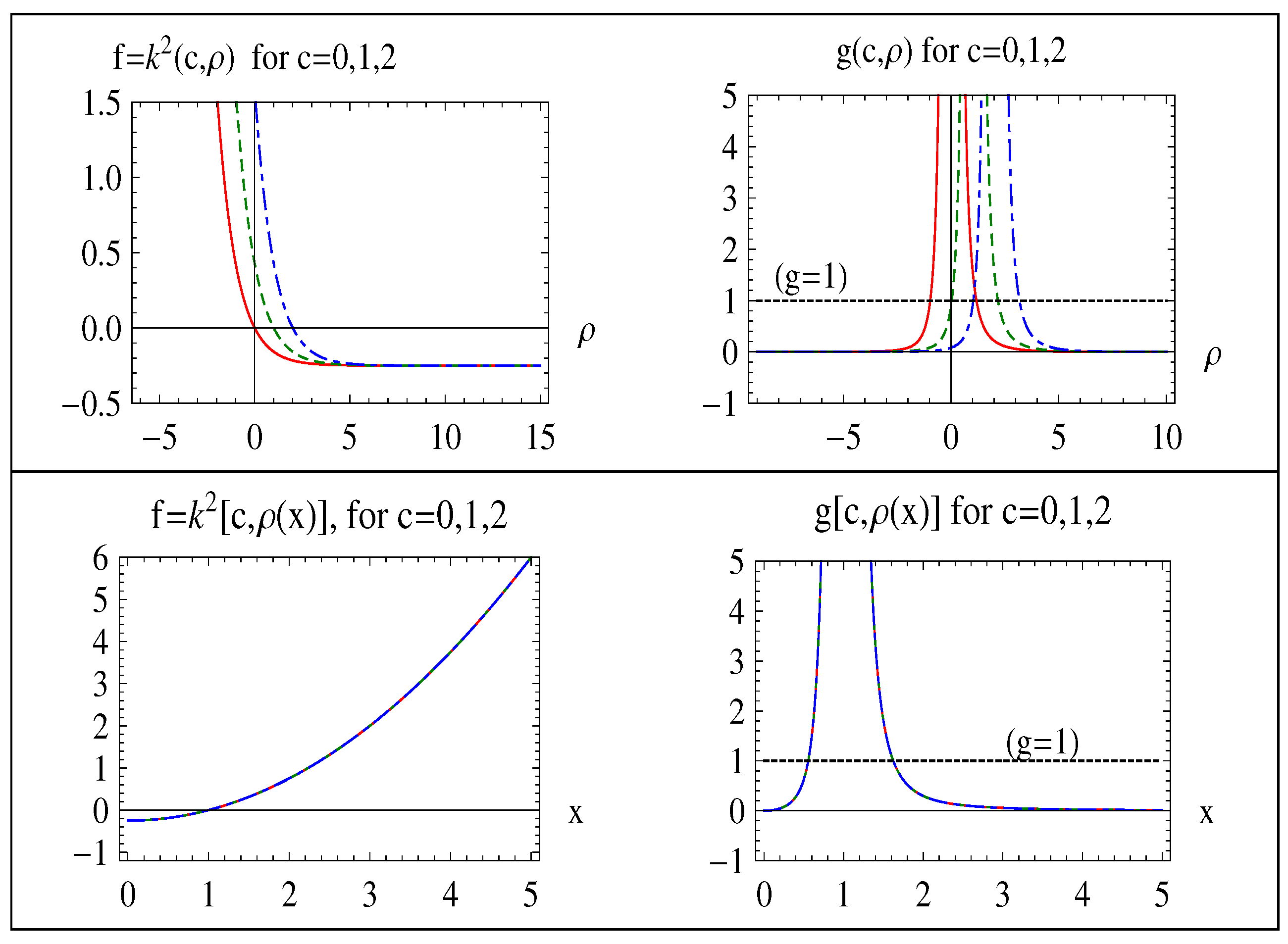
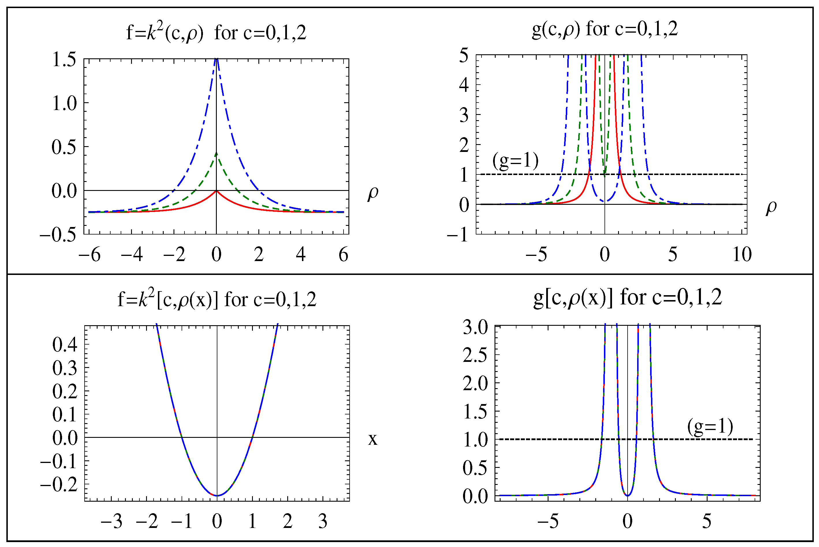
In other words, one cannot expect to have accurate ${\left(JWKB\right)}_1$ solutions in the region(s) where the inequality condition (26) does not hold (since the potential in the TISE gets sharper and higher order ${\left(JWKB\right)}_{n>1}$ approximation is required [3,4,5]). If this inequality holds, it corresponds to $\rho \in S{D}_1$, and otherwise, it corresponds to $\rho \in S{D}_2$ regarding the discussion in the Introduction section. Calculation of $g(c,\rho )$ in (26) for the ${\left(BDE\right)}_1$ with (17b) gives:

$$0\le g(c,\rho )=\frac{1}{4}{e}^{Re(\rho +c)}\left|\frac{4e^{\rho }+e^c}{e^{\rho }-e^c}\right|<<1,$$

(27)

whose graph with the graph of $f(c,\rho )$ for some c values is given in Figure 1. We see that the classical turning point where $f(c,\rho )=0$ is at ${\rho }_t=c$, the CIR where $f(c,\rho )<0$ lies on the right-hand side of this turning point and the CAR where $f(c,\rho )>0$ lies on the left-hand-side of it. Therefore, we know in advance from (3) and (4) that we should make the asymptotic matching (modification) in the CIR (since it is located at the RHS of the turning point (${\rho }_t=c$)) as follows [3,4]:

$$y^{m.}(c,\rho )\to \underset{\rho \to \infty }{lim}y(c,\rho )=0,$$

(28a)

$${\tilde{y}}^{m.}(c,\rho )\to \underset{\rho \to \infty }{lim}\tilde{y}(c,\rho )=0.$$

(28b)

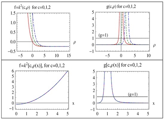
Figure 1. Graph of f and g functions for some c values (solid red curve: $c=0$; dotted green: $c=1$; dashed blue: $c=2$).

Moreover, a narrow subregion not obeying (27) for each c value in the domain cannot be expected to give accurate results by the ${\left(JWKB\right)}_1$ method since it is lying at just about the turning points (as a typical property of the ${\left(JWKB\right)}_1$ method, as mentioned above). Analysis of such regions in need of higher order JWKB approximation (${\left(JWKB\right)}_{N>1}$) are beyond the scope of our study.

The width of this narrow sub-region (corresponding to $S{D}_2$ discussed in the Introduction section) can be found from the solution of $g(c,\rho )$ in (27) for real ρ and c values as follows:

$$S{D}_2:\rho \in (c-0.968889,c+1.17808).$$

(29a)

The remaining wide region (corresponding to $S{D}_1$ discussed in the Introduction section):

$$S{D}_1:-\infty <\rho <<(c-0.968889)\cup (c+1.17808)<<\rho <\infty$$

(29b)

is our main concern for a good-enough ${\left(JWKB\right)}_1$ general solution here.

In the ${\left(JWKB\right)}_1$ calculations, the entire domain can be considered as a unification of two neighboring regions (CAR-CIR), and if we start with the CAR located at the left-hand side of the turning point and connect it to the CIR by using the conventional ${\left(JWKB\right)}_1$ connection formulas given in [3,4,5] in the reverse direction, we find the same formulas for $y_L(c,\rho )$ and $y_R(c,\rho )$ as in ([4] (see Example 1)) (but in $(c,\rho )$ in this section, rather than $(c,x)$) to give:

$$\tilde{y}(c,\rho )=\left\{\begin{array}{c}{\tilde{y}}_L(c,\rho ),\mathrm{for}-\infty <\rho \le c\\ {\tilde{y}}_R(c,\rho ),\mathrm{for}c\le \rho <\infty \end{array}\right.,$$

(30)

where:

$${\tilde{y}}_L(c,\rho )=\frac{A\left(c\right)}{\sqrt{k(c,\rho )}}sin[\eta (c,\rho )+\alpha \left(c\right)],$$

(31a)

and:

$$y_R(c,\rho )=\frac{A\left(c\right)}{2\sqrt{\kappa (c,\rho )}}cos\left[\alpha \left(c\right)-\pi /4\right]e^{\left[-\zeta (c,\rho )\right]}+\frac{A\left(c\right)}{\sqrt{\kappa (c,\rho )}}sin\left[\alpha \left(c\right)-\pi /4\right]e^{\left[\zeta (c,\rho )\right]}.$$

(31b)

The constituent functions, η and ζ, in (31a) and (31b) now give:

$$\begin{array}{c}\eta (c,\rho )={\int }_{\rho }^{c}k(c,\rho )d\rho =\sqrt{e^{c-\rho }-1}+i[\frac{\rho -c}{2}+ln\left(\sqrt{1-e^{c-\rho }}\right)+1],\rho <c\hfill \\ \zeta (c,\rho )={\int }_c^{\rho }\kappa (c,\rho )d\rho =-\frac{c}{2}-\sqrt{1-e^{c-\rho }}+ln[e^{\rho /2}+\sqrt{e^{\rho }-e^c}],c<\rho \hfill \end{array}$$

(32a)

(where k and κ have the usual meanings: ${\kappa }^2=-k^2$), and the c dependent coefficients can be found from the applications of the initial values given in (21) as follows:

$$\left[\begin{array}{c}\tilde{y}(c,d_2)=y_L(c,d_2)={\alpha }_2\left(c\right)\hfill \\ {\partial }_{\rho }\tilde{y}(c,\rho ){|}_{\rho =d_2}={\partial }_{\rho }{y}_L(c,\rho ){|}_{\rho =d_2}={\beta }_2\left(c\right)\hfill \end{array}\right]{|}_{\left\{\begin{array}{c}{d}_2=0\\ {\alpha }_2\left(c\right)=0\\ {\beta }_2\left(c\right)=1\end{array}\right\}}$$

(32b)

$$\Rightarrow \left\{\begin{array}{c}A\left(c\right)=\frac{-\sqrt{2}}{{(e^c-1)}^{1/4}}(\mathrm{for}0<c<\infty )\hfill \\ \alpha \left(c\right)=\frac{ic}{2}-\sqrt{e^c-1}-iln(1+\sqrt{1-e^c}),0<c<\infty \hfill \end{array}\right..$$

(32c)

Note that $\tilde{y}(c,d_2)$ in (32b) corresponds to $y_L(c,d_2)$ according to (30), since the initial values are chosen at $\rho =d_2$, which is in the CAR: $-\infty <d_2=0<c$. The ${\left(JWKB\right)}_1$ general solution in the other form given in (20), which is very important in our analysis, can similarly be written as follows [3,4]:

$$\begin{array}{c}{\tilde{y}}_1(c,\rho )=\left\{\begin{array}{c}\frac{2}{\sqrt{k(c,\rho )}}sin[\eta (c,\rho )+\pi /4],-\infty <\rho \le c\hfill \\ \frac{1}{\sqrt{\kappa (c,\rho )}}exp[-\zeta (c,\rho )],c\le \rho <\infty \hfill \end{array}\right.\end{array}$$

$${\tilde{y}}_2(c,\rho )=\left\{\begin{array}{c}\frac{1}{\sqrt{k(c,\rho )}}sin[-\eta (c,\rho )+\pi /4],-\infty <\rho \le c\hfill \\ \frac{1}{\sqrt{\kappa (c,\rho )}}exp\left[\zeta (c,\rho )\right],c\le \rho <\infty \hfill \end{array}\right.,$$

(33)

where $\eta (c,\rho )$ and $\zeta (c,\rho )$ are given in (32a), and applications of the initial values in (18) give:

$$\left\{\begin{array}{c}\tilde{y}(c,d_2)={\tilde{c}}_1\left(c\right){\tilde{y}}_1(c,d_2)+{\tilde{c}}_2\left(c\right){\tilde{y}}_2(c,d_2)={\alpha }_2\left(c\right)\hfill \\ {\left[{\partial }_{\rho }\tilde{y}(c,\rho )\right]}_{\rho =d_2}={\left[\begin{array}{cc}& {\tilde{c}}_1\left(c\right){\partial }_{\rho }{\tilde{y}}_1(c,\rho )\hfill \\ & +{\tilde{c}}_2\left(c\right){\partial }_{\rho }{\tilde{y}}_2(c,\rho )\hfill \end{array}\right]}_{\rho =d_2}={\beta }_2\left(c\right)\hfill \end{array}\right.,$$

(34)

whose solutions for the c-dependent coefficients via the applications of the initial values in (21) give:

$$\begin{array}{c}\hfill {\tilde{c}}_1\left(c\right)=\frac{{\alpha }_2\left(c\right){\partial }_{\rho }{\tilde{y}}_2(c,\rho )\left|{}_{\rho =d_2}\right.-{\beta }_2\left(c\right){\tilde{y}}_2(c,d_2)}{\tilde{\Delta }(c,d_2)}{|}_{\left\{\begin{array}{c}{d}_2=0\\ {\alpha }_2\left(c\right)=0\\ {\beta }_2\left(c\right)=1\end{array}\right\}}\\ \hfill =-\frac{cos\left[\pm i\frac{c}{2}+\sqrt{e^c-1}\mp iln(1+\sqrt{1-e^c})+\frac{\pi }{4}\right]}{\sqrt{2}{(e^c-1)}^{1/4}},\end{array}$$

(35a)

$$\begin{array}{c}\hfill {\tilde{c}}_2\left(c\right)=\frac{-{\alpha }_2\left(c\right){\partial }_{\rho }{\tilde{y}}_1(c,\rho )\left|{}_{\rho =d_2}\right.-{\beta }_2\left(c\right){\tilde{y}}_1(c,d_2)}{\tilde{\Delta }(c,d_2)}{|}_{\left\{\begin{array}{c}{d}_2=0\\ {\alpha }_2\left(c\right)=0\\ {\beta }_2\left(c\right)=1\end{array}\right\}}\\ \hfill =\frac{\sqrt{2}sin\left[\pm i\frac{c}{2}+\sqrt{e^c-1}\mp iln(1+\sqrt{1-e^c})+\frac{\pi }{4}\right]}{{(e^c-1)}^{1/4}},\end{array}$$

(35b)

where the discriminant $\tilde{\Delta }(c,d)$ (the Wronskian determinant) is similarly defined by:

$$\tilde{\Delta }(c,d_2)=\left|\begin{array}{cc}{\tilde{y}}_1(c,d_2)& {\tilde{y}}_2(c,d_2)\\ \frac{\partial }{\partial \rho }{\tilde{y}}_1(c,\rho )\left|{}_{\rho =d_2}\right.& \frac{\partial }{\partial \rho }{\tilde{y}}_2(c,\rho )\left|{}_{\rho =d_2}\right.\end{array}\right|.$$

(36)

Remark 1.

Note that choosing either ${\alpha }_2$ or ${\beta }_2$ zero as we do here in (21) obviously simplifies the calculations of the coefficients in the ${\left(JWKB\right)}_1$ general solutions (see Equations (35a) and (35b)).

3.2. Asymptotic Matching of the ${\left(BDE\right)}_1$ in the Normal Form

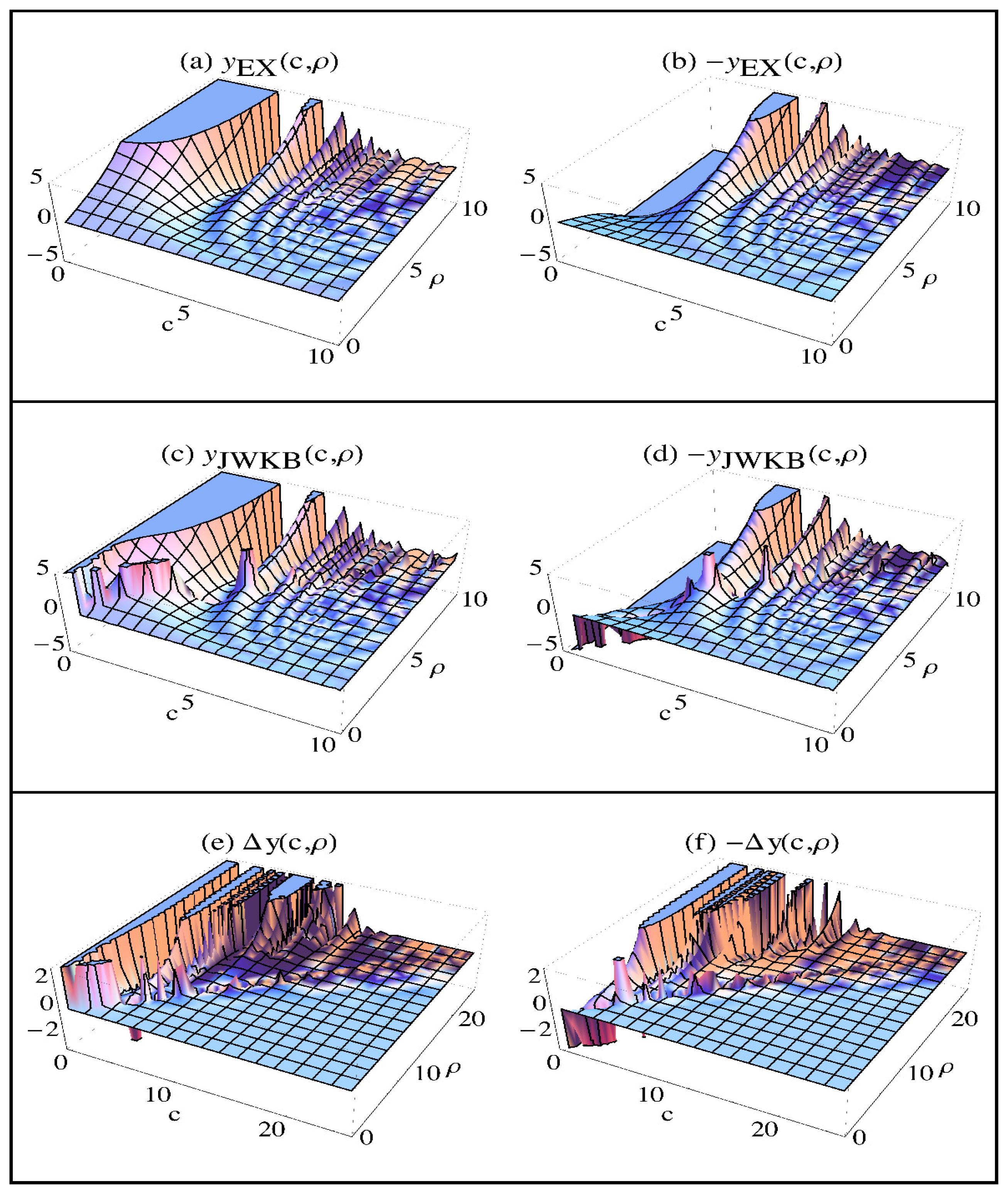
Results of our unmatched calculations are given in Figure 2. 3D graphs here are cut at appropriate planes for a better view as much as possible. We can see that ${\left(JWKB\right)}_1$ solutions diverge at some turning points where $\rho =c$. However, we would see it for the missing turning points (as a typical property of ${\left(JWKB\right)}_1$ solutions for all of the classical turning points) if they were cut at smaller heights, but then the visible ones in Figure 2 would be suppressed since their divergence width and divergence tendency are different for different $\rho =c$ values. What we are interested is that ${\left(JWKB\right)}_1$ solutions here are consistent with the exact solutions in the CAR where $-\infty <\rho <c$, but asymptotically are not (as ρ increases in the CIR where $c<\rho <\infty$) as expected. Now, the question is whether we can see this without either interference of the exact solutions (we did it in Figure 2 for now) or consulting the present asymptotic matching rules given in (3) and (4) (it gives (28b) here) and under what conditions they can be asymptotically-matched (in other words, what the asymptotic matching rule is).

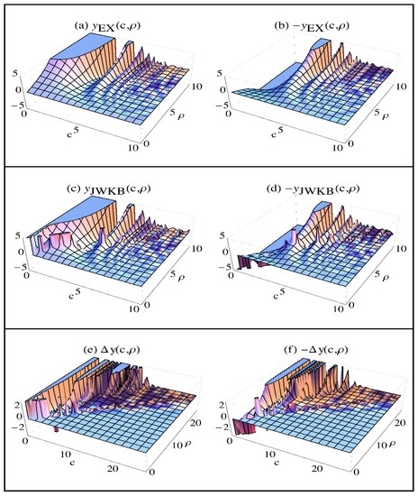
Figure 2. Results of the normal form ${\left(JWKB\right)}_1$ solutions: 3D graphs of: (a) $y_{EX}(c,\rho )$; (b) $-y_{EX}(c,\rho )$; (c) $y_{JWKB}(c,\rho )$; (d) $-y_{JWKB}(c,\rho )$; (e) $\Delta y(c,\rho )=y_{EX}(c,\rho )-y_{JWKB}(c,\rho )$; (f) $-\Delta y(c,\rho )=-[y_{EX}(c,\rho )-y_{JWKB}(c,\rho )]$.

From the JWKB theories, we know that the formal expression of the ${\left(JWKB\right)}_N$ approximation written in (5) takes the form:

$${\tilde{y}}_N(c,\rho )=exp\left[\frac{1}{\delta }\sum _{n=0}^N{\delta }^n{S}_n(c,\rho )\right],(\delta \to 0)$$

(37)

where the first three of them can be written in $(c,\rho )$ as follows [3,4]:

$$\begin{array}{cc}\hfill S_0(c,\rho )& =\pm \int \sqrt{{\kappa }^2(c,\rho )}d\rho =:\pm A_0(c,\rho )=\left\{\begin{array}{c}{S}_{01}(c,\rho )=-A_0(c,\rho )\hfill \\ S_{02}(c,\rho )=A_0(c,\rho )\hfill \end{array}\right.,\hfill \end{array}$$

(38a)

$$\begin{array}{cc}\hfill S_1(c,\rho )& =-\frac{1}{4}ln{\kappa }^2(c,\rho )=:A_1(c,\rho )=\left\{\begin{array}{c}{S}_{11}(c,\rho )=A_1(c,\rho )\hfill \\ S_{12}(c,\rho )=A_1(c,\rho )\hfill \end{array}\right.,\hfill \end{array}$$

(38b)

$$\begin{array}{cc}\hfill S_2(c,\rho )& =\pm \int \left\{\frac{{\partial }^2\left[{\kappa }^2(c,\rho )\right]/\partial {\rho }^2}{8{\kappa }^3(c,\rho )}-\frac{5\partial \left[{\kappa }^2(c,\rho )\right]/\partial \rho }{32{\kappa }^5(c,\rho )}\right\}d\rho \hfill \\ & =:\pm A_2(c,\rho )=\left\{\begin{array}{c}{S}_{21}(c,\rho )=-A_2(c,\rho )\hfill \\ S_{22}(c,\rho )=A_2(c,\rho )\hfill \end{array}\right.,\hfill \end{array}$$

(38c)

where ${\kappa }^2=-k^2$ has the usual meaning. Here, in $S_{ij}$, the first index $i=0,1,2$ represents the first three JWKB expansion terms, and the second index $j(=$$1,2)$ represents two different sets due to the two-valuedness of these expansion terms as in [4]. For the ${\left(JWKB\right)}_1$ approximation, only the first two terms ($n=0$ and up to $N=1$ only) in (37) are used to give the well-known ${\left(JWKB\right)}_1$ formula in $(c,\rho )$ as follows:

$$\left.\begin{array}{c}{\tilde{y}}_1(c,\rho )=exp[\frac{S_{01}(c,\rho )}{\delta }+S_{11}(c,\rho )]\hfill \\ {\tilde{y}}_2(c,\rho )=exp[\frac{S_{02}(c,\rho )}{\delta }+S_{12}(c,\rho )]\hfill \end{array}\right\},\delta \to 0,$$

(39)

which is equivalent to (33). As discussed above, according to (28b), the ${\left(JWKB\right)}_1$ solution in the CIR requires a cancellation of either ${\tilde{y}}_1$ or ${\tilde{y}}_2$ in Equation (20) for the subdomain where the ${\left(JWKB\right)}_1$ applicability criterion holds (in $S{D}_1$). Note that both the exact solution in (22) and the ${\left(JWKB\right)}_1$ solution in (33) involve asymptotically diverging exponential terms in the CIR. As a result, this modification can fulfill the physical requirement, according to which the corresponding quantum mechanical system in the normal form (the TISE) does not allow any asymptotically diverging term in the CIR (in both the exact and ${\left(JWKB\right)}_1$ solution) [3,4,5].

Semiclassically, a successful (accurate with respect to the exact solution) ${\left(JWKB\right)}_1$ solution of the TISE should have asymptotically-descending ${\left(JWKB\right)}_1$ expansion terms with indices $n=0$ and $n=1$, and they should be bounded by the next term with index $n=2$ (which is not involved in the ${\left(JWKB\right)}_1$ solution, though) [3,4]. These requirements can be written by considering $\delta \to =1$ to give [4]:

$$1>>\delta S_2<S_1<S_0/\delta ,\delta \to =1.$$

(40)

Due to the two-valuedness, we can write the following proposition to determine which term (${\tilde{y}}_1$ or ${\tilde{y}}_2$) exhibits the asymptotic requirements:

Proposition 2.

In order to be an accurate ${\left(JWKB\right)}_1$ solution (and hence, in order to be a properly asymptotically-matched ${\left(JWKB\right)}_1$ solution), the general JWKB expansion terms should satisfy the following inequalities:

$$\begin{array}{c}\hfill 1>>{\tilde{S}}_{21}(c,\rho or\rho \left(x\right))<{\tilde{S}}_{11}(c,\rho or\rho \left(x\right))<{\tilde{S}}_{01}(c,\rho or\rho \left(x\right)),\end{array}$$

(41a)

$$\begin{array}{c}\hfill 1>>{\tilde{S}}_{22}(c,\rho or\rho \left(x\right))<{\tilde{S}}_{12}(c,\rho or\rho \left(x\right))<{\tilde{S}}_{02}(c,\rho or\rho \left(x\right)),\end{array}$$

(41b)

where the definition of ${\tilde{S}}_{ij}$ in [4] can be generalized (so as to involve also the transformed representation of our model ${\left(BDE\right)}_1$ under study) as follows:

$${\tilde{S}}_{ij}(c,\rho or\rho \left(x\right))=\left\{\begin{array}{c}\left|S_{ij}(c,\rho or\rho \left(x\right))\right|,if{S}_{ij}(c,\rho or\rho \left(x\right))\in \mathbb{C}\\ S_{ij}(c,\rho or\rho \left(x\right)),if{S}_{ij}(c,\rho or\rho \left(x\right))\in \mathbb{R}\end{array}\right..$$

(42)

Proof. 

Expansion terms in a specific problem (depending on the corresponding $f(c,\rho or\rho (x\left)\right)$ (where $f(c,\rho or\rho (x\left)\right)⟺f(c,\rho )$ or $f(c,\rho (x\left)\right)$)) in (17a) may give real or complex $S_{ij}(c,\rho or\rho \left(x\right))$ (where $S_{ij}(c,\rho or\rho \left(x\right))⟺S_{ij}(c,\rho )$ or $S_{ij}(c,\rho \left(x\right))$) functions in various (sub)domains. Therefore, the requirements given in (41a) and (41b), which are the natural consequence of (40) exhibiting a successful comparison according to their two-valuedness, make the proof complete. ☐

Corollary 1.

The expansion term(s) in the ${\left(JWKB\right)}_1$ solutions ($S_{01}$, $S_{02}$, $S_{11},$ and $S_{12}=S_{11}$) in (39) (building (33) for the ${\left(BDE\right)}_1$), whose associated ${\tilde{S}}_{ij}(c,\rho )$ or ${\tilde{S}}_{ij}(c,\rho \left(x\right))$ elements determined from (42) do not obey (41a) and (41b), should be canceled for successful asymptotic modification.

Inequalities in (41a) and (41b) and the definition in (42) can freely be used in both representations independently, and what we have for the transformed coordinates in $(c,\rho )$, which is also our main concern here, becomes:

$${\tilde{S}}_{ij}(c,\rho )=\left\{\begin{array}{c}\left|S_{ij}(c,\rho )\right|,\rho <c\because S_{ij}(c,\rho )\in \mathbb{C}\mathrm{in}\mathrm{the}\mathrm{CAR}\hfill \\ S_{ij}(c,\rho ),c<\rho \because S_{ij}(c,\rho )\in \mathbb{R}\mathrm{in}\mathrm{the}\mathrm{CIR}\hfill \end{array}\right.,$$

(43)

since from (38a)–(38c), we have:

$$\begin{array}{cc}& S_{01}(c,\rho )=-S_{02}(c,\rho )=\hfill \\ & -\frac{\sqrt{1-e^{c-\rho }}[-2\sqrt{e^{\rho }-e^c}+\rho e^{\rho /2}+2e^{\rho /2}ln(1+e^{-\rho /2}\sqrt{e^{\rho }-e^c})]}{2\sqrt{e^{\rho }-e^c}},\hfill \end{array}$$

(44a)

$$\begin{array}{cc}& S_{11}(c,\rho )=S_{12}(c,\rho )=-\frac{1}{4}ln(\frac{1-e^{c-\rho }}{4}),\hfill \end{array}$$

(44b)

$$\begin{array}{cc}& S_{21}(c,\rho )=-S_{22}(c,\rho )=\frac{-6e^c-4e^{\rho }}{48\sqrt{1-e^{c-\rho }}(e^{\rho }-e^c)},\hfill \end{array}$$

(44c)

from which we see that $S_{ij}(c,\rho )\in \mathbb{C}$ in the CAR (where $\rho <c$) and $S_{ij}(c,\rho )\in \mathbb{R}$ in the CIR (where $c<\rho$)). It should be noted here in advance that the result of the application of (42) for the re-transformed representation, $(c,x)$, will be different than that in (43) of the $(c,\rho )$ system (see Section 4). In order to make the comparison given in (41a) and (41b), we determine whether the elements are real or complex similar to [4]. Therefore, the general expression (also including the SLP case in [4]) for the asymptotic matching can be written by (41a), (41b) and (42) as the generalized asymptotic matching rule. If both (41a) and (41b) hold (we obviously see that this happens in the CAR), then the ${\left(JWKB\right)}_1$ general solution involves both ${\left(JWKB\right)}_1$ complementary functions (${\tilde{y}}_1$ and ${\tilde{y}}_2$). However, if either of them does not hold (we obviously see this in the CIR), then the related complementary ${\left(JWKB\right)}_1$ function not obeying (either ${\tilde{y}}_1$ or ${\tilde{y}}_2$) should cancel in the ${\left(JWKB\right)}_1$ general solution for that non-obedient domain. This generalization involves also the SLP case in [4] where there is no such subdomain, but a non-obedient domain (corresponding to the CIR). Note that (39) with (38a)–(38c) has an implication that $S_{i1}$ (and hence, ${\tilde{S}}_{i1}$) contributes to ${\tilde{y}}_1$, whereas $S_{i2}$ (and hence, ${\tilde{S}}_{i2}$) contributes to ${\tilde{y}}_2$. Therefore, the non-obedient $S_{i1}$ terms require a cancellation of ${\tilde{y}}_1$, and similarly, non-obedient $S_{i2}$ terms require a cancellation of ${\tilde{y}}_2$ in the related subdomains.

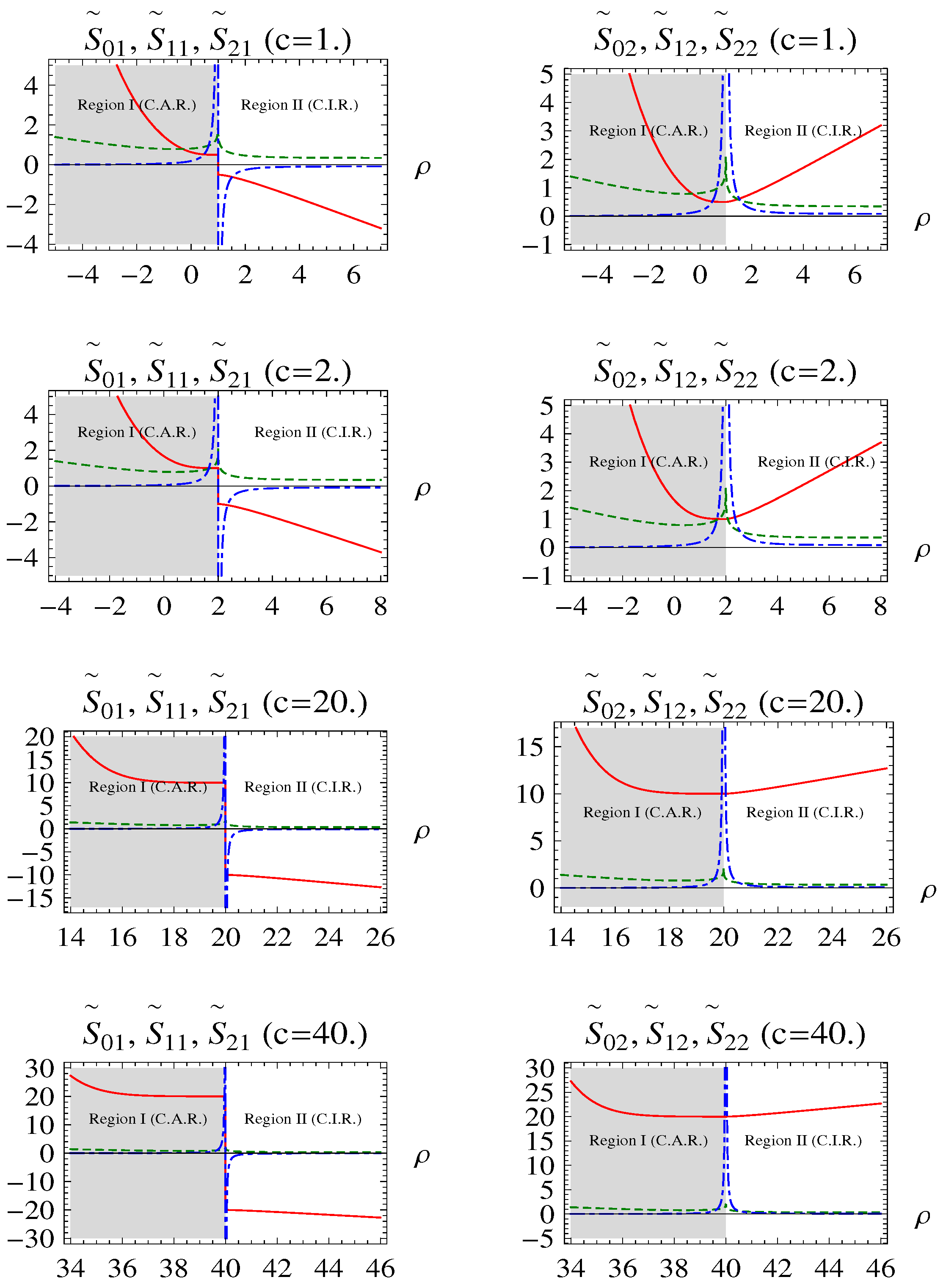
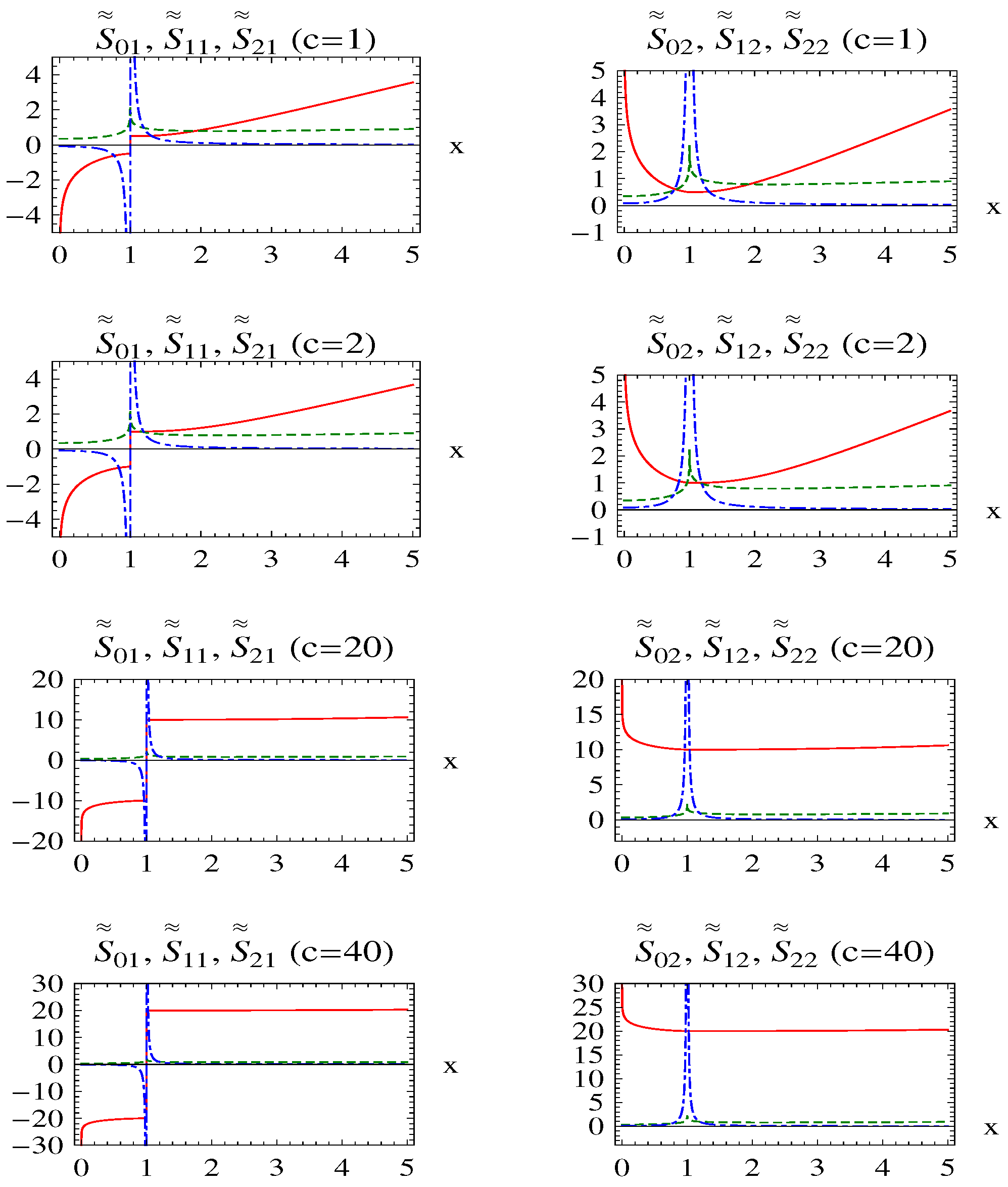
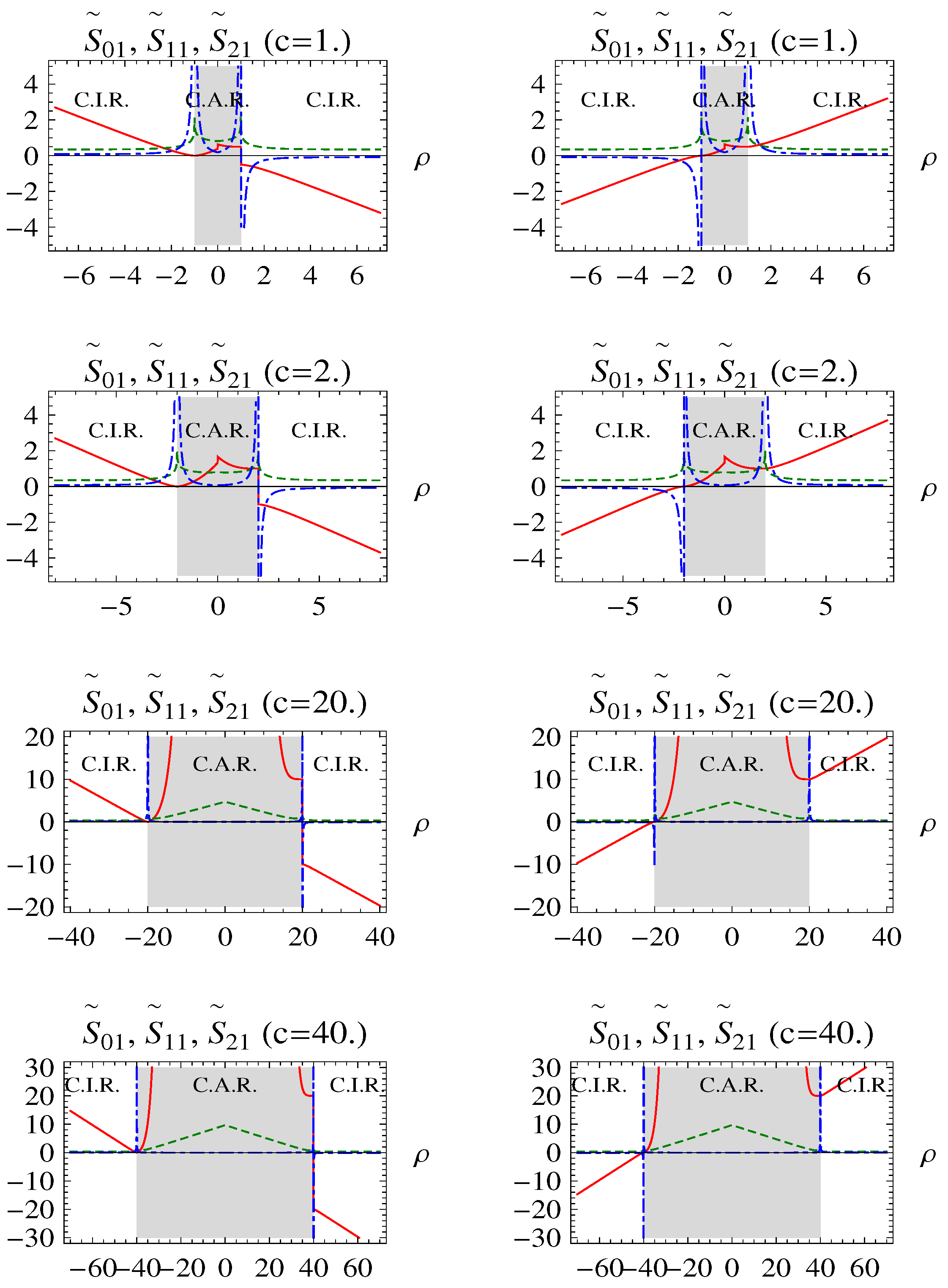
Graphs of the ${\tilde{S}}_{i1}(c,\rho )$ and ${\tilde{S}}_{i2}(c,\rho )$ for some c values are given in Figure 3. Comparing with the graph of $g(c,\rho )$ given in Figure 1, we can see that ${\left(JWKB\right)}_1$ solutions should be consistent with the exact solutions except for the non-obedient narrow regions given by (29a). We can also see that both (41a) and (41b) hold for the CAR, whereas the CIR does not hold for both and, hence, needs a cancellation in the non-obedient ${\tilde{S}}_{i1}$ term (left column graphs) in this region ($c<\rho <\infty$). This is the most remarkable consequence of our pure ${\left(JWKB\right)}_1$ analysis via Figure 3 without any interference of either the exact solutions or physical nature of the corresponding quantum mechanical system. In Figure 3, we have non-obedient ${\tilde{S}}_{i1}$ functions, requiring a cancellation of $S_{i1}$, which contributes to $\widetilde{y_1}$ (exhibiting exponentially-increasing behavior) in the CIR.

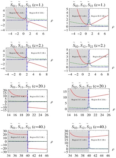
Figure 3. Graphs of ${\tilde{S}}_{i,j=1}$ (left column) and ${\tilde{S}}_{i,j=2}$ (right column) (where$i=0,1,2$) in the normal form in $(c,\rho )$ for some specific c values (solid-red curves: $f or$ $i=0$; dotted-green curves: $f ori=1$; and dashed-blue curves: $f ori=2$).

As a result, the necessary modifications according to our pure semiclassical analyses for the asymptotic matching of the ${\left(BDE\right)}_1$ in the transformed normal form representation should be as follows:

• Modification of the exact general solution in (22) (which will be used to compare with the modified ${\left(JWKB\right)}_1$ solutions):

  $$y^{(m.)}(c,\rho )=\left\{\begin{array}{c}y,-\infty <\rho \le c\left(CAR\right)\hfill \\ c_1\left(c\right)J_1(e^{\frac{c-\rho }{2}}),c\le \rho <\infty \left(CIR\right)\hfill \end{array}\right..$$

  (45)
  Note that both exact and ${\left(JWKB\right)}_1$ solutions in (22) and (31b) of (30) (or (33) of (20)) have the common form of exponentially-increasing terms in the CIR, $c<\rho <\infty$, where a cancellation according to (41a), (41b) and (42) is required for both exact and ${\left(JWKB\right)}_1$ solutions (see also (47a) below for a comparison).
• Modification of the ${\left(JWKB\right)}_1$ general solution in (30):

  $${\tilde{y}}^{(m.)}(c,\rho )=\left\{\begin{array}{c}{\tilde{y}}_L,\mathrm{for}-\infty <\rho \le c\left(CAR\right)\\ {\tilde{y}}_R^{(m.)},\mathrm{for}c\le \rho <\infty \left(CIR\right)\end{array}\right.,$$

  (46a)

  where:

  $${\tilde{y}}_R^{(m.)}(c,\rho )=\frac{A\left(c\right)}{2\sqrt{\kappa (c,\rho )}}cos\left[\alpha \left(c\right)-\pi /4\right]Exp\left[-\zeta (c,\rho )\right].$$

  (46b)
• Modification of the ${\left(JWKB\right)}_1$ general solution in the other form (see Equation (20) via (33)):

  $${\tilde{y}}^{(m.)}(c,\rho )={\tilde{c}}_1\left(c\right){\tilde{y}}_1(c,\rho )+{\tilde{c}}_2\left(c\right){\tilde{y}}_2^{(m.)}(c,\rho ),$$

  (47a)

  where:

  $${\tilde{y}}_2^{(m.)}(c,\rho )=\left\{\begin{array}{c}\frac{1}{\sqrt{k(c,\rho )}}sin[-\eta (c,\rho )+\pi /4],-\infty <\rho \le c\left(CAR\right)\hfill \\ 0,c\le \rho <\infty \left(CIR\right)\hfill \end{array}\right..$$

  (47b)

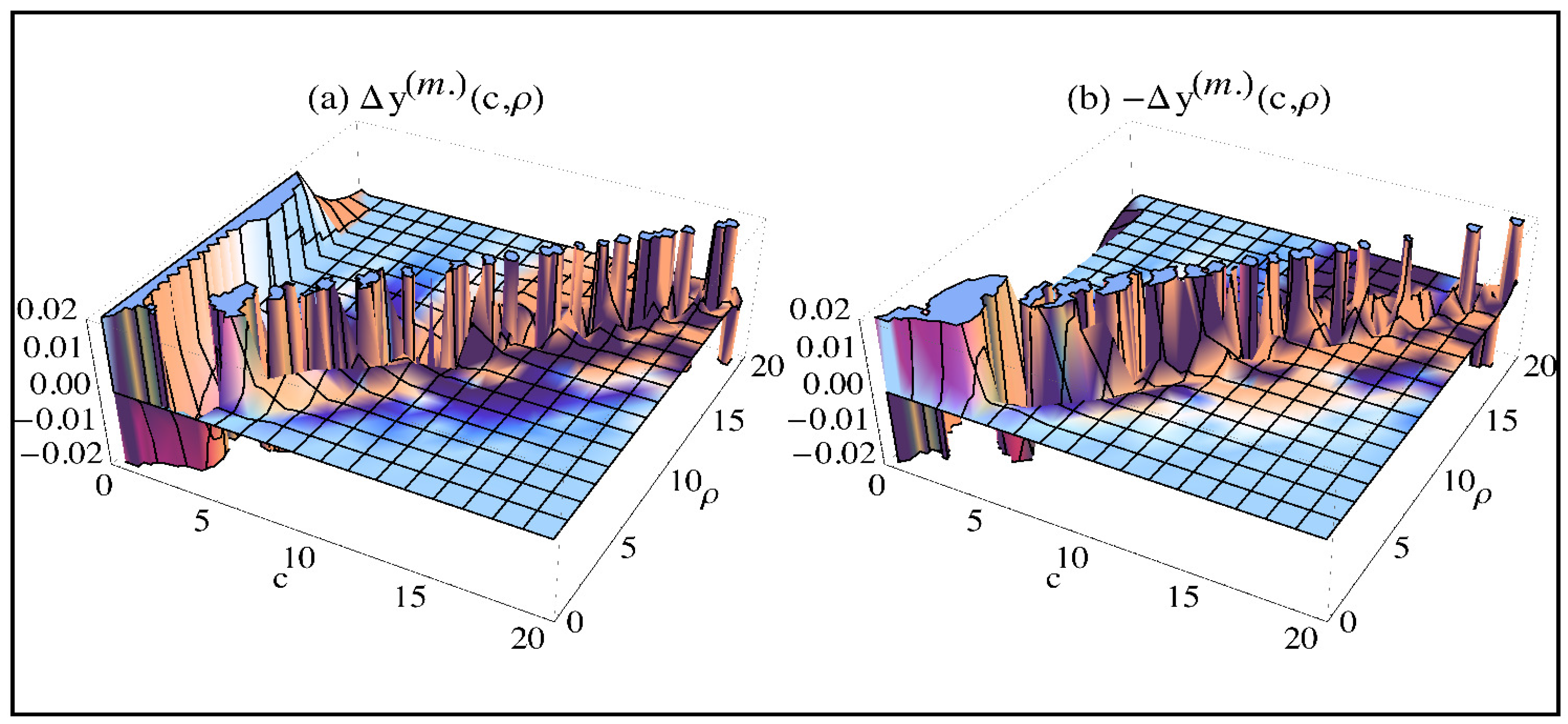
The superscript “(m.)” shows successfully asymptotically-matched solutions here. Error graphs in 3D given in Figure 4 show the success of these asymptotic matchings when compared with the error graphs in Figure 2e,f. These asymptotic modifications are the results of our generalized asymptotic matching rules suggested here in (41a), (41b) and (42), which is a semiclassical establishment of the existing asymptotic matching rules in (28a) and (28b) (or (3) and (4)). Therefore, they can be used as an alternative, more general and pure semiclassical (without interfering either exact solutions or physical nature of the system) asymptotic modification rules. It is now clear that after the modification, the anomalies in the CIR have been removed successfully for the subdomain where the ${\left(JWKB\right)}_1$ applicability criterion holds according to (29b) as has been aimed by the asymptotic modification (matching) process.

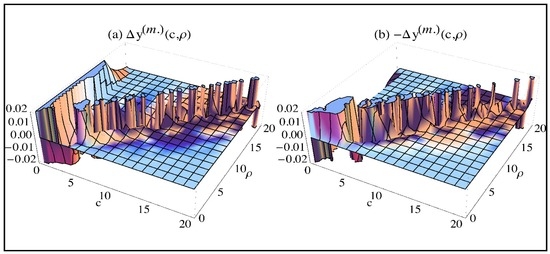
Figure 4. 3D error graphs of asymptotically-modified normal form ${\left(JWKB\right)}_1$ general solutions: (a) $\Delta y^{m.}(c,\rho )=y_{EX}^{m.}(c,\rho )-y_{JWKB}^{m.}(c,\rho )$; (b) $-\Delta y^{m.}(c,\rho )=-[y_{EX}^{m.}(c,\rho )-y_{JWKB}^{m.}(c,\rho )]$.

4. Calculations in the Standard Form

4.1. Exact and ${\left(JWKB\right)}_1$ Solutions of the ${\left(BDE\right)}_1$ in the Standard Form

One can obviously find the exact general solutions in the re-transformed variable representation, in $(c,x)$, either by substituting (12) in the reverse form:

$$\rho :(0,\infty )\to (-\infty ,\infty ),\rho \left(x\right)=c-2lnx$$

(48)

in (22) or, alternatively, by directly solving (7) with the following associated initial values in (9) (see also Remark 2 for the relations of the initial values in both equivalent representations):

$$\{\begin{array}{c}y\left(x\right)\left|{}_{x=d_1=e^{c/2}}\right.={\alpha }_1\left(c\right)=0\hfill \\ y^{\prime }\left(x\right)\left|{}_{x=d_1=e^{c/2}}\right.={\beta }_1\left(c\right)=-2e^{-c/2}\hfill \end{array},$$

(49)

where prime denotes derivative with respect to x.

Note that implicitly equivalent definitions: $y(c,x)=:y(c,\rho (x\left)\right)$, $f(c,x)=:f(c,\rho (x\left)\right)$ and $g(c,x)=:g(c,\rho (x\left)\right)$ can be used to refer to the functions $y,f,$ or g expressed in variables c and x; however, it is clear that they are actually not equal to each other explicitly, i.e., ${f(c,\rho \left(x\right))=f(c,\zeta )|}_{\zeta \to \rho \left(x\right)}{\ne f(c,\zeta )|}_{\zeta \to x}=f(c,x)$. Therefore, explicit definitions in $(c,x)$ are shown with a double tilde for ${\tilde{S}}_{ij}$ as given in Equation (52) (see the notations in Equations: (42) and (52) for a comparison).

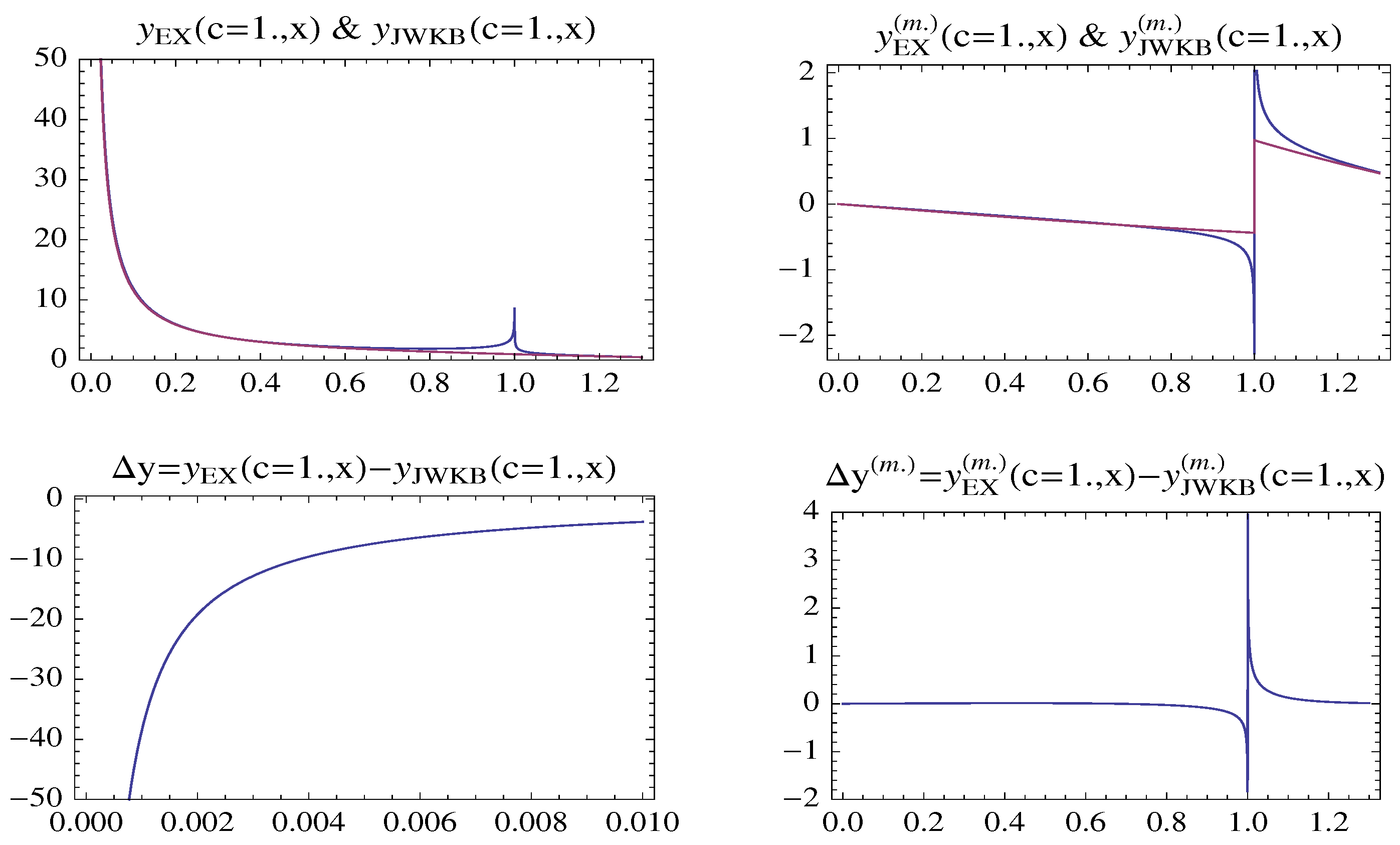
Although y in the latter case is in single variable (in x only), we have the general solution of the associated IVP in two variables (in $(c,x)$) as required since the corresponding initial values in (49) are c-dependent to give both x and c-dependent y results in the exact general solution. However, we do not have two alternatives for finding an accurate general solution by the ${\left(JWKB\right)}_1$ method since this method is not appropriate for the ${\left(BDE\right)}_1$ in the standard form given in (7) as discussed above. Therefore, in order to find the ${\left(JWKB\right)}_1$ general solution in the standard form representation in $(c,x)$, we have to substitute (48) into the ${\left(JWKB\right)}_1$ general solution obtained in the transformed (normal form) representation (in $(c,\rho )$) in (30) (or (20) for the other form) with the related c-dependent coefficients given in (32c) (or (35a) and (35b) for the other form). In other words, $y_{JWKB}(c,x)=:y_{JWKB}{[c,\rho \left(x\right)]=y(c,\zeta )|}_{\zeta \to \rho \left(x\right)}$. Now, both exact and ${\left(JWKB\right)}_1$ solutions are consistent in the domain of x except for a small region around $x=1$ ($S{D}_2$). It is the typical property of the ${\left(JWKB\right)}_1$ method discussed above since $\rho =c$ is the classical turning point where $f(c,\rho )$ in Equations (17a) and (17b) is zero, and it corresponds to $x=1$ (since $li{m}_{\rho \to c}x\left(\rho \right)=li{m}_{\rho \to c}{e}^{(c-\rho )/2}=1$ for $\forall c\in \mathbb{R}$).

Moreover, a detailed analysis shows also the following: according to the graph of $f[c,\rho (x\left)\right]$ and $g[c,\rho (x\left)\right]$ in Figure 1, the CIR involves the subdomain, $0<x<1$ for $\forall c\in \mathbb{R}$, where we should have the inaccurate ${\left(JWKB\right)}_1$ solution, but that can be asymptotically matched by the asymptotic matching rules we have suggested in (41a), (41b) and (42), since this subregion lies within the region where the ${\left(JWKB\right)}_1$ applicability criterion holds ($S{D}_1$). For the unmodified solutions, we can see that we really have inaccurate ${\left(JWKB\right)}_1$ solutions as expected in this CIR, and we can consider it in two subregions: as $x\to 1$ and as $x\to 0$, roughly. From Figure 1, we see that the ${\left(JWKB\right)}_1$ method is useless as $x\to 1$, since $li{m}_{x\to 1}g[c,\rho \left(x\right)]>1$, and hence, the ${\left(JWKB\right)}_1$ applicability criterion does not hold ($S{D}_2$). However, for the other subregion as $x\to 0$, we have $li{m}_{x\to 0}g[c,\rho \left(x\right)]<1$, where we can expect to have accurate ${\left(JWKB\right)}_1$ solutions ($S{D}_1$), provided that some successful asymptotic modification is applied. Let us determine these two subdomains ($S{D}_1$ and $S{D}_2$) corresponding to the CIR more precisely: the non-obedient narrow region for the ${\left(JWKB\right)}_1$ method around $\rho =c$ given in (29a) corresponds to (via (48)):

$$x\in (0.554858,1.62327)for\forall c\in \mathbb{R}.$$

(50a)

Similarly, the obedient region (for the ${\left(JWKB\right)}_1$ approximation) given in (29b) in ρ corresponds to (via (48)):

$$0<x<<0.554858\cup 1.62327<<x<\infty for\forall c\in \mathbb{R},$$

(50b)

where we can obtain accurate ${\left(JWKB\right)}_1$ solutions if we make a proper asymptotic matching. In other words, we have two subdomains (or literally, related subregions: $S{R}_1$ and $S{R}_2$):

• $S{D}_1:0<x<<0.554858$ (appropriate for the ${\left(JWKB\right)}_1$) and
• $S{D}_2:0.554858<x<1$ (inappropriate for the ${\left(JWKB\right)}_1$)

where $CIR=S{D}_1\cup S{D}_2$, and we are interested in $S{D}_1$ in our ${\left(JWKB\right)}_1$ analysis since the ${\left(JWKB\right)}_1$ applicability criterion holds for it. Therefore, we can obviously apply the asymptotic matching rules suggested in (41a), (41b) and (42) to modify the CIR: $0<x<1$, so that we can obtain accurate results (as we should do according to the consequence of the ${\left(JWKB\right)}_1$ applicability criterion in Equation (50b)). 3D graphs regarding our standard form solutions are given in Figure 5 (see the anomalies around $x=0$ and $x=1$ as shown above). The asymptotically-matchable narrow subdomain $S{D}_1$ is studied in the next subsection.

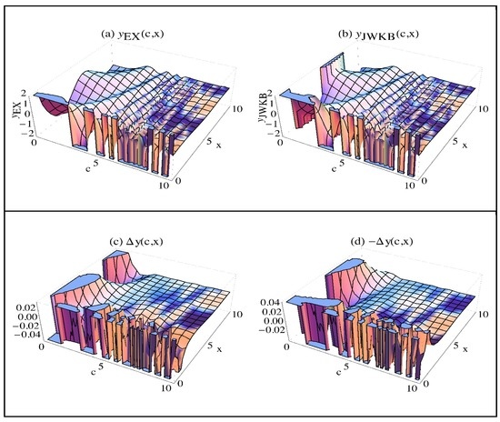
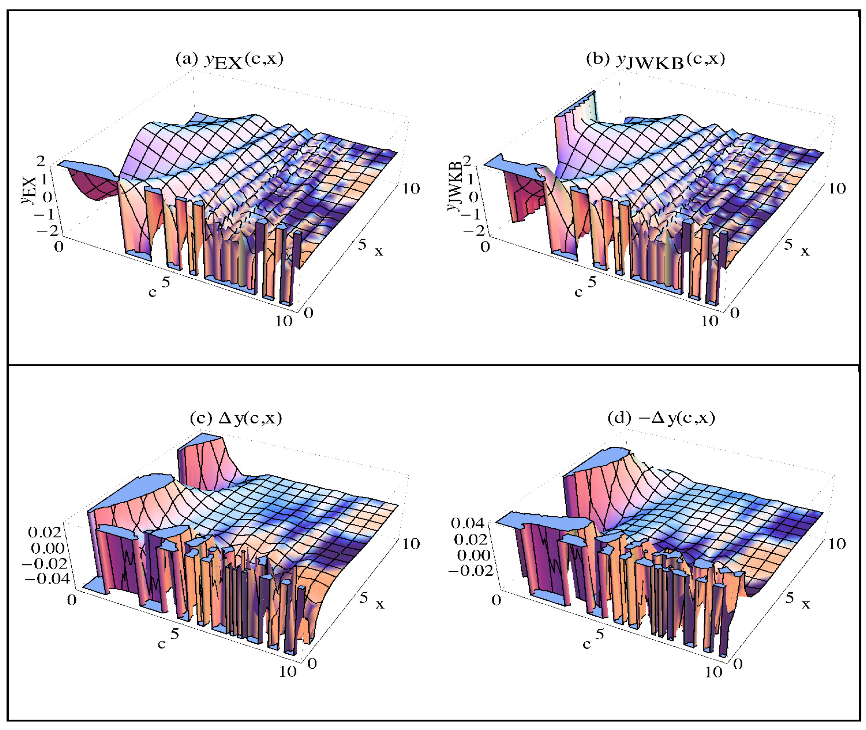
Figure 5. Results of the standard form ${\left(JWKB\right)}_1$ solutions: 3D graphs of: (a) $y_{EX}(c,x)$; (b) $y_{JWKB}(c,x)$; (c) $\Delta y(c,x)=y_{EX}(c,x)-y_{JWKB}(c,x)$; (d) $-\Delta y(c,x)=-[y_{EX}(c,x)-y_{JWKB}(c,x)]$.

4.2. Asymptotic Matching of the ${\left(BDE\right)}_1$ in the Standard Form

Since $li{m}_{\rho \to \infty }x=0^{+}$, we can directly write the modifications for the asymptotic matching given in (28a) and (28b) (via (4)) in x coordinates as follows:

For the general exact solution:

$$y_{EX}^{(m.)}[c,\rho \left(x\right)]=y^{m.}[c,\rho \left(x\right)]=:y_{EX}^{(m.)}[c,\rho \left(x\right)]\to \underset{x\to 0^{+}}{lim}{y}_{EX}[c,\rho \left(x\right)]=0.$$

(51a)

For the general ${\left(JWKB\right)}_1$ solution:

$$y_{{\left(JWKB\right)}_1}^{(m.)}[c,\rho \left(x\right)]={\tilde{y}}^{m.}[c,\rho \left(x\right)]=:{\tilde{y}}^{m.}(c,x)\to \underset{x\to 0^{+}}{lim}{y}_{JWKB}[c,\rho \left(x\right)]=0.$$

(51b)

Another way to do the right asymptotic modification in the x-system, which is our main concern as a pure semiclassical asymptotic matching here, is sure to use the reverse transformation in (48) via the asymptotically-modified results in the ρ-system obtained in (45), (46a) and (47a). However, for now, let us apply our asymptotic matching rules to see the accuracy of the ${\left(JWKB\right)}_1$ solution directly in the x-system. If the results obtained in the $(c,x)$-system are accurate (or inaccurate), we should also see it by the suggested asymptotic matching rules in (41a), (41b) and (42).

A careful inspection shows that, substitution of (48) in the $S_{ij}(c,\rho )$ results (in Equations (44a)–(44c)) gives complex $S_{ij}(c,\rho \left(x\right))$ functions for both CAR and CIR. Therefore, the expression of ${\tilde{S}}_{ij}(c,\rho \left(x\right))$ in (42) simply gives:

$${\tilde{\tilde{S}}}_{ij}(c,x)\to {\tilde{S}}_{ij}(c,\rho \left(x\right))=\left|S_{ij}(c,\rho \left(x\right))\right|,\mathrm{for}allx\in \mathbb{R}$$

(52)

which is obviously different than what was found in (43) for the $(c,\rho )$ system even obtained by the use of the same definition in (42). Here, we used the double tilde to represent the $\tilde{S}$ function in the re-transformed coordinates, namely ${\tilde{\tilde{S}}}_{ij}(c,x)={\tilde{S}}_{ij}{(c,\zeta )|}_{\zeta \to \rho \left(x\right)}={\tilde{S}}_{ij}(c,\rho \left(x\right))$, since they would not be equal to each other mathematically if we used both with the same function name (${\tilde{S}}_{ij}(c,x)\ne {\tilde{S}}_{ij}(c,\rho \left(x\right))$.

We can now test the conditions in (41a) and (41b) in $(c,x)$ coordinates to see whether our ${\left(JWKB\right)}_1$ general solution needs asymptotic matching somewhere according to our ${\tilde{S}}_{ij}$-based semiclassical analysis without interference of the exact solutions. Graphs of the ${\tilde{\tilde{S}}}_{i1}(c,x)$ and ${\tilde{\tilde{S}}}_{i2}(c,x)$ for some specific c values are given in Figure 6 from which we can see that final ${\left(JWKB\right)}_1$ solutions in $(c,x)$ do not need asymptotic modification in $1<x<\infty$ (since both ${\tilde{\tilde{S}}}_{i1}(c,x)$ and ${\tilde{\tilde{S}}}_{i2}(c,x)$ obey (41a) and (41b) via the use of (42) in this region). However, the non-obedient ${\tilde{\tilde{S}}}_{i1}(c,x)$ terms (and hence, ${\tilde{y}}_1$ in (2b)), which should be removed from the ${\left(JWKB\right)}_1$ general solution in the $S{D}_1$ (for a successful asymptotic matching), are clearly seen in the graphs given in Figure 6. In other words, according to the asymptotic matching rules suggested here (in Equations (41a) and (41b) via the use of (42)), we necessarily have to do the following asymptotic modifications for a correct asymptotic matching:

$${\tilde{y}}^{(m.)}(c,x)=:{\tilde{y}}^{(m.)}(c,\rho \left(x\right))={\tilde{c}}_1\left(c\right){\tilde{y}}_1(c,\rho \left(x\right))+{\tilde{c}}_2\left(c\right){\tilde{y}}_2^{(m.)}(c,\rho \left(x\right))$$

(53a)

where:

$${\tilde{y}}_2^{(m.)}(c,\rho \left(x\right))=\left\{\begin{array}{c}\frac{1}{\sqrt{k(c,\rho (x\left)\right)}}sin[-\eta (c,\rho \left(x\right))+\frac{\pi }{4}],1.62327<<x<\infty (\subset CAR)\hfill \\ 0,0<x<0.554858(\subset CIR)\hfill \end{array}\right.$$

(53b)

which is similarly equivalent to (51b). Remember that $S{D}_2$ lying inside the $CIR$ cannot be asymptotically matched as discussed above.

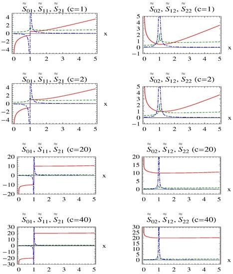
Figure 6. Graphs of ${\tilde{\tilde{S}}}_{i,j=1}$ (left column) and ${\tilde{\tilde{S}}}_{i,j=2}$ (right column) (where$i=0,1,2$) in the standard form in $(c,x)$ for a specific c value, $c=1$, (solid-red curves: $f or$ $i=0$; dotted-green curves: $f ori=1$; and dashed-blue curves: $f ori=2$).

Similarly,

$$y^{(m.)}(c,x)=:\left\{\begin{array}{c}y(c,\rho (x\left)\right),1.62327<<x<\infty (\subset CAR)\\ y^{(m.)}(c,\rho \left(x\right)),0<x<0.554858(\subset CIR)\end{array}\right.$$

(54a)

where $y(c,\rho (x\left)\right)$ can be written by the substitution of (48) in (22) to give:

$$\begin{array}{c}y(c,\rho \left(x\right))=c_1\left(c\right)J_1\left(x\right)+c_2\left(c\right)Y_1\left(x\right),\hfill \\ y^{(m.)}(c,\rho \left(x\right))=c_1\left(c\right)J_1\left(x\right)\hfill \end{array}$$

(54b)

which is equivalent to (51a). Results showing the enhancement in our asymptotic matching for the standard form representation are given in Figure 7 for a specific case of $c=1$.

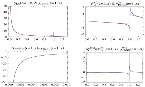
Figure 7. Enhancement in the standard form ${\left(JWKB\right)}_1$ solution by our asymptotic modifications in the $S{D}_1$ for $c=1$.

Remark 2.

Point $d_2$ at which the initial values are defined in the $(c,\rho )$ representation (normal form) with (18)–(21) corresponds to $d_1$ at which the initial values are defined in the original $(c,x)$ system (standard form) with (9)–(49) via the change of variable given in (12) or (48). Therefore, $d_1$, $d_2$ and, hence, the initial values in both representations have the following relations:

From (48),

$$d_2\in (-\infty ,\infty )\to d_1=exp(\frac{c-d_2}{2})\in (0,\infty )$$

(55)

and consequently,

$$\begin{array}{c}\hfill {\left[y\left(x\right)={\alpha }_1\left(c\right)\right]}_{x=d_1}={\left[y\left(\rho \right)={\alpha }_2\left(c\right)\right]}_{\rho =d_2}\\ \hfill \Rightarrow \begin{array}{|c|}\hline {\alpha }_1\left(c\right)={\alpha }_2\left(c\right)\\ \hline\end{array},\end{array}$$

(56a)

$$\begin{array}{c}\hfill \frac{dy\left(x\right)}{dx}{|}_{x=d_1}={\beta }_1\left(c\right)=\frac{dy\left(\rho \right)}{d\rho }\frac{d\rho \left(x\right)}{dx}{|}_{x=d_1}\\ \hfill =-{\left[\frac{2}{x}{\beta }_2\left(c\right)\right]}_{x=d_1}\Rightarrow \begin{array}{|c|}\hline {\beta }_1\left(c\right)=-{\left[\frac{2}{x}{\beta }_2\left(c\right)\right]}_{x=d_1}\\ \hline\end{array}.\end{array}$$

(56b)

One can check that initial values chosen (in (18)–(21) and (49)) also exhibit this relationship.

5. A Physical Application: Exponential Potential Decorated Bound State Problem

It might be interesting to test the success of our alternative asymptotic matching rules in a real quantum mechanical (physical) problem corresponding to the normal form representation via the TISE. Therefore, let us apply these calculations to a specific case of the exponential potential decorated bound state problem studied in [10], from which we have the followings (note that we use different symbols here so that we can refer to the calculations in this work, namely: $\{\psi ,x,X,y\}$ in [10] are replaced by $\{y,\tau ,\rho ,x\}$ here, respectively):

For the TISE in (1a) and (1b), but in variable τ, the potential under study is given by:

$$V\left(\tau \right)=-V_0{e}^{-\alpha \left|\tau \right|}=\left\{\begin{array}{c}-V_0{e}^{-\alpha \tau },0\ge \tau \\ -V_0{e}^{\alpha \tau },0\le \tau \end{array}\right.(V_0>0,\alpha >0,E<0,-\infty <\tau <\infty ).$$

(57)

Necessarily, $E<0$ for the bound states and by a simple change of variable:

$$\rho =\alpha \tau ,$$

(58)

we have the TISE in (1a) and (1b) in ρ:

$$V\left(\rho \right)=-V_0{e}^{-\left|\rho \right|}=\left\{\begin{array}{c}-V_0{e}^{-\rho },0\ge \rho \\ -V_0{e}^{\rho },0\le \rho \end{array}\right.(V_0>0,E<0,-\infty <\rho <\infty ).$$

(59)

Now, the definitions of dimensionless a and b:

$$a=\sqrt{\frac{8m{V}_0}{{\hslash }^2{\alpha }^2}}\mathrm{and}b=\sqrt{\frac{-8mE}{{\hslash }^2{\alpha }^2}}$$

(60)

give the TISE in ρ with:

$$f(a,b,\rho )=\left\{\begin{array}{c}{f}_1\left(a,b,\rho \ge 0\right)=\frac{a^2{e}^{-\rho }-b^2}{4}\\ f_2\left(a,b,\rho \le 0\right)=\frac{a^2{e}^{\rho }-b^2}{4}\end{array}\right..$$

(61)

Then, the change of the independent variable:

$$x=a{e}^{-\rho /2}$$

(62)

gives the b-th order Bessel differential equation, ${\left(BDE\right)}_b$, namely:

$$y^{″}+\frac{1}{x}{y}^{\prime }+\frac{(x^2-b^2)}{x^2}y=0$$

(63)

whose exact general solution is the linear combination of two kinds of the b-th order Bessel functions (similar to (19a) and (19b)), namely:

$$\left\{\begin{array}{c}{y}_{EX}(a,b,\rho \ge 0)=c_1^{+}\left(a\right)J_b\left(a{e}^{-\rho /2}\right)+c_2^{+}\left(a\right)Y_b\left(a{e}^{-\rho /2}\right)\hfill \\ y_{EX}(a,b,\rho \le 0)=c_1^{-}\left(a\right)J_b\left(a{e}^{\rho /2}\right)+c_2^{-}\left(a\right)Y_b\left(a{e}^{\rho /2}\right)\hfill \end{array}\right..$$

(64)

Note that, second complementary solutions for both regions in (64) are given in [10] (instead of $Y_b(a{e}^{\rho /2})$) as $J_{-b}(a{e}^{\rho /2})$, since $J_b(a{e}^{\rho /2})$ and $J_{-b}(a{e}^{\rho /2})$ are two linearly independent solutions for non-integer Bessel functions (just like $J_b(a{e}^{\rho /2})$ and $Y_b(a{e}^{\rho /2})$). Indeed, from Bessel theories, we have [13,14]:

$$Y_b\left(x\right)=\left\{\begin{array}{c}\underset{p\to b}{lim}\frac{J_p\left(x\right)cos\left(p\pi \right)-J_{-p}\left(x\right)}{sin\left(p\pi \right)},ifb\in \mathbb{Z}\hfill \\ \frac{J_b\left(x\right)cos\left(b\pi \right)-J_{-b}\left(x\right)}{sin\left(b\pi \right)},ifb\notin \mathbb{Z}\hfill \end{array},\right.$$

(65)

and for also integer b values, as in our study here with $b=1$, we can use Equation (64) as a general expression involving both integer and non-integer b values [13,14]. Now, (22) takes the form:

$$\left\{\begin{array}{c}{y}_{EX}(c,\rho \ge 0)=c_1^{+}\left(c\right)J_1(e^{\frac{c-\rho }{2}})+c_2^{+}\left(c\right)Y_1(e^{\frac{c-\rho }{2}})\hfill \\ y_{EX}(c,\rho \le 0)=c_1^{-}\left(c\right)J_1(e^{\frac{c+\rho }{2}})+c_2^{-}\left(c\right)Y_1(e^{\frac{c+\rho }{2}})\hfill \end{array}\right.,$$

(66)

and its comparison with (64) gives the following relation:

$$\left.\begin{array}{c}a{e}^{-\rho /2}=e^{\frac{c-\rho }{2}},\rho \ge 0\\ a{e}^{\rho /2}=e^{\frac{c+\rho }{2}},\rho \le 0\end{array}\right\}\Rightarrow \begin{array}{|c|}\hline a=\sqrt{e^c}\\ \hline\end{array}.$$

(67)

Now, let us take $b=1$ as a special case and apply the asymptotic matching rules we have already found in the previous sections. Our restriction then becomes:

$$b=1\to E_n=-\frac{{\hslash }^4{\alpha }^4}{16m^2},$$

(68)

so that we have:

$$f(c,\rho )=f(a,b,\rho ){|}_{\left\{\begin{array}{c}a\to \sqrt{e^c}\hfill \\ b\to 1\hfill \end{array}\right\}}=\left\{\begin{array}{c}{f}_1\left(c,\rho \ge 0\right)=\frac{e^{c-\rho }-1}{4}\\ f_2\left(c,\rho \le 0\right)=\frac{e^{c+\rho }-1}{4}\end{array}\right.,$$

(69)

which is just as the form we have been using here as in (17a) and (17b). Additionally, its solution from (64) gives:

$$\begin{array}{c}\hfill y(c,\rho )=y(a,b,\rho ){|}_{\left\{\begin{array}{c}a\to \sqrt{e^c}\hfill \\ b\to 1\hfill \end{array}\right\}}=\left\{\begin{array}{c}y(c,\rho \ge 0)=c_1^{+}\left(c\right)J_1(e^{\frac{c-\rho }{2}})+c_2^{+}\left(c\right)Y_1(e^{\frac{c-\rho }{2}})\\ y(c,\rho \le 0)=c_1^{-}\left(c\right)J_1(e^{\frac{c+\rho }{2}})+c_2^{-}\left(c\right)Y_1(e^{\frac{c+\rho }{2}})\end{array}\right.\end{array}$$

(70)

which is just the same as our result in (22). Our intention here is not to find accurate ${\left(JWKB\right)}_1$ eigenenergies ($E_n$) and eigenfunctions (${\tilde{y}}_n$) where some correction terms (like Friedrich-Trost (F-T) corrections) are involved [8,11,12], but to apply our asymptotic matching rules under the assumption in (68) where the problem simplifies to the ${\left(BDE\right)}_1$ being studied here.

Conventional asymptotic modification rules in (4) were applied in [10] to give:

$$y(\tau \to \pm \infty )=y(a,b,\rho \to \pm \infty )=0\Rightarrow c_2^{+}\left(a\right)=c_2^{-}\left(a\right)=0,$$

(71a)

which means:

$$y(c,\rho \to \pm \infty )=0\Rightarrow c_2^{+}\left(c\right)=c_2^{-}\left(c\right)=0$$

(71b)

in our calculations. We have already shown half of it for $f(c,\rho )=f_1(c,\rho ),\rho \ge 0$ by our alternative semiclassical asymptotic matching rule in (41a), (41b) and (42) via Figure 3, but let us see it for (69) in the whole domain explicitly:

Now, expansion terms in (38a)–(38c) for (69) give just the same as (44a)–(44c) for $\rho \ge 0$, but these results require $\rho \to -\rho$ for $\rho \le 0$, namely:

$$\begin{array}{cc}& S_{01}(c,\rho )=-S_{02}(c,\rho )=\hfill \\ & \left\{\begin{array}{c}-\frac{\sqrt{1-e^{c-\rho }}[-2\sqrt{e^{\rho }-e^c}+\rho e^{\rho /2}+2e^{\rho /2}ln(1+e^{-\rho /2}\sqrt{e^{\rho }-e^c})]}{2\sqrt{e^{\rho }-e^c}},\rho \ge 0\hfill \\ -\frac{\sqrt{1-e^{c+\rho }}[-2\sqrt{e^{-\rho }-e^c}-\rho e^{-\rho /2}+2e^{-\rho /2}ln(1+e^{\rho /2}\sqrt{e^{-\rho }-e^c})]}{2\sqrt{e^{\rho }-e^c}},\rho \le 0\hfill \end{array}\right.,\hfill \end{array}$$

(72a)

$$\begin{array}{cc}& S_{11}(c,\rho )=S_{12}(c,\rho )=\left\{\begin{array}{c}-\frac{1}{4}ln(\frac{1-e^{c-\rho }}{4}),\rho \ge 0\hfill \\ -\frac{1}{4}ln(\frac{1-e^{c+\rho }}{4}),\rho \le 0\hfill \end{array}\right.,\hfill \end{array}$$

(72b)

$$\begin{array}{cc}& S_{21}(c,\rho )=-S_{22}(c,\rho )=\left\{\begin{array}{c}\frac{-6e^c-4e^{\rho }}{48\sqrt{1-e^{c-\rho }}(e^{\rho }-e^c)},\rho \ge 0\hfill \\ \frac{-6e^c-4e^{-\rho }}{48\sqrt{1-e^{c+\rho }}(e^{-\rho }-e^c)},\rho \le 0\hfill \end{array}\right.,\hfill \end{array}$$

(72c)

from which (42) gives:

$${\tilde{S}}_{ij}(c,\rho )=\left\{\begin{array}{c}\left|S_{ij}(c,\rho )\right|,\mathrm{for}\left|\rho \right|<c(\mathrm{since}{S}_{ij}(c,\rho )\in \mathbb{C}\mathrm{in}\mathrm{the}\mathrm{CAR})\\ S_{ij}(c,\rho ),\mathrm{for}c<\left|\rho \right|(\mathrm{since}{S}_{ij}(c,\rho )\in \mathbb{R}\mathrm{in}\mathrm{the}\mathrm{CIR})\end{array}\right..$$

(73)

Graphs of functions f and g in both representations are given in Figure 8, from which we can see that ${\left(JWKB\right)}_1$ solutions are consistent with the exact solutions, except for the non-obedient narrow regions (from (29a)):

$$\left|\rho \right|\in (c-0.968889,c+1.17808),$$

(74a)

and the remaining wide regions (from (29b)):

$$-\infty <\left|\rho \right|<<(c-0.968889)\cup (c+1.17808)<<\left|\rho \right|<\infty$$

(74b)

need asymptotic matching ($S{D}_1$). Graphs of ${\tilde{S}}_{i1}(c,\rho )$ and ${\tilde{S}}_{i2}(c,\rho )$ for some c values are given in Figure 9. We can obviously see that both (41a) and (41b) hold in the CAR simultaneously, but they do not hold in the CIR simultaneously and, hence, are in need of a cancellation in the CIR. Here, we have non-obedient ${\tilde{S}}_{i1}$ term (and hence, a cancellation of ${\tilde{y}}_1)$ for $0<c<\rho <\infty$ (see the left column in Figure 9) and ${\tilde{S}}_{i2}$ term (and hence, a cancellation of ${\tilde{y}}_2$) for $-\infty <\rho <-c<0$ (see the right column in Figure 9) in these CIRs. This is because, as stated above, (39) with (38a)–(38c) has an implication that $S_{i1}$ (or ${\tilde{S}}_{i1}$) contributes to ${\tilde{y}}_1$ and $S_{i2}$ (or ${\tilde{S}}_{i2}$) contributes to ${\tilde{y}}_2$. Therefore, the non-obedient $S_{i1}$ terms requiring a cancellation of ${\tilde{y}}_1$ for $0<c<\rho <\infty$ and $S_{i2}$ terms requiring a cancellation of ${\tilde{y}}_2$ for $-\infty <\rho <-c<0$ give the same right asymptotic matching as given in (71b) of [10].

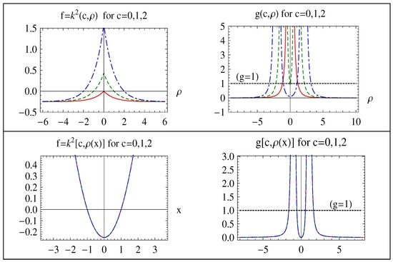
Figure 8. Graph of f and g functions of the exponential potential decorated bound state problem for some c values (solid-red curves: $c=0$; dotted-green curves: $c=1$; dashed-blue curves: $c=2$). First row: normal form representation corresponding to the Time Independent Schrodinger’s Equation (TISE); second row: standard form representation corresponding to the ${\left(BDE\right)}_1$.

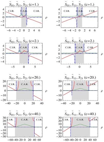
Figure 9. Graphs of ${\tilde{S}}_{i,j=1}$ (left column) and ${\tilde{S}}_{i,j=2}$ (right column) (where $i=0,1,2$) of the exponential potential decorated bound state problem (which corresponds to the normal form representation via the TISE with the related exponential potential) under study in the normal form representation in $(c,\rho )$ for some specific c values (solid-red curves: $f or$ $i=0$; dotted-green curves: $f ori=1$; and dashed-blue curves: $f ori=2$).

6. Conclusions

In this work, the ${\left(BDE\right)}_1$ has been chosen as a mathematical model for a pure semiclassical analysis (without interference of the physical nature of the system) since there exist subdomains where the ${\left(JWKB\right)}_1$ applicability criterion both holds (in $S{D}_1$) and fails (in $S{D}_2$). The hereby presented generalized asymptotic matching rules regarding the ${\tilde{S}}_{ij}$ matrix elements obtained from the ${\left(JWKB\right)}_N$ expansion terms show that the ${\left(JWKB\right)}_1$ general solution of the ${\left(BDE\right)}_1$ for carefully chosen initial values needs asymptotic matching in the transformed (normal form) representation in the CIR where the ${\left(JWKB\right)}_1$ applicability criterion holds ($S{D}_1$). Moreover, there is no need for asymptotic matching in the CAR where the ${\left(JWKB\right)}_1$ applicability criterion holds (again $S{D}_1$). These results, obtained by our pure semiclassical analysis, are consistent with the present conventional asymptotic matching rules given in (3) and (4) via [3,4], which is a natural consequence of the physical nature of the related quantum mechanical system (the normalizability requirement of quantum mechanical wave functions). The generalized asymptotic matching rules suggested in (41a) and (41b) with the generalized definition of ${\tilde{S}}_{ij}$ in (42) are the results of our pure semiclassical analyses where the physical nature of the system is not interfered.

As explained in the work in detail, physics (nature) requires asymptotic matching to the full mathematical solution. Physical systems of second order are generally of two kinds:

$$\begin{array}{c}\hfill \left(\mathrm{i}\right)IVP:y^{″}+f\left(\rho \right)y=0,y^{\prime }\left({\rho }_0\right)=k_1,y\left({\rho }_0\right)=k_2\\ \hfill \left(\mathrm{ii}\right)BVP:y^{″}+f\left(\rho \right)y=0,y\left({\rho }_0\right)=k_1,y\left({\rho }_0\right)=k_2\end{array}$$

(here, both are given in the normal form). We have two initial values or boundary values for both as common. However, physics require a third initial value or a third boundary value (or more correctly, an asymptotic constraint) given in (3) and (4), which is called asymptotic matching since $x_0\to \pm \infty$ in (4). In this work, it is studied and proven mathematically via the JWKB theories stating that JWKB expansion terms should be descending and bounded as given and studied in [3,4]. Therefore, the main idea here is the semiclassical requirement that ${\left(JWKB\right)}_N$ expansion terms should be asymptotically decreasing as the term index increases and bounded by the $(N+1)$-th indexed term as stated in [3,4]. The two valuedness of the ${\left(JWKB\right)}_N$ expansion terms as given in (38a)–(38c) enables definitions of two different sets (corresponding to two complementary functions as in (39)) according to (42) for them so that the semiclassical requirements for the asymptotic matching can be tested for these two sets accordingly. Equation (39) shows that $S_{i1}$ (hence, ${\tilde{S}}_{i1}$ in our comparison function) contributes to ${\tilde{y}}_1$, and similarly, $S_{i2}$ (hence, ${\tilde{S}}_{i2}$ in our comparison function) contributes to ${\tilde{y}}_2$. Therefore, any violation of ${\tilde{S}}_{i1}$ in (41a) requires a cancellation of ${\tilde{y}}_1$, and any violation of ${\tilde{S}}_{i2}$ in (41b) requires a cancellation of ${\tilde{y}}_2$ in the related non-obedient (sub)domain provided that the ${\left(JWKB\right)}_1$ applicability criterion holds (=$S{D}_1$). The same definition in (42) gives (43) in the transformed normal form representation and (52) in the re-transformed standard form representation, respectively. When they are used in our alternative asymptotic matching rules given in (41a) and (41b), this gives consistent results with the present asymptotic matching rules given in (3) and (4). Moreover, our alternative analyses enable a correct determination of which complementary function (solution) and where in the semiclassically solvable (sub)domain to cancel. As a result, asymptotic matching rules suggested here gives enhanced ${\left(JWKB\right)}_1$ solutions for the specifically chosen ${\left(BDE\right)}_1$ in both normal form and standard form representations. Since both standard and normal forms correspond to different sub-domains obeying the JWKB applicability criterion in (6) and (29b) being for the normal form and (50b) being for the standard form), both should require different asymptotic matching results for these different domains. In deed, our suggested asymptotic matching rule has explained both correctly and has given the correct results as the existing asymptotic matching rules given in (3) and (4). Applications of our pure semiclassical asymptotic matching rules to the exponential potential decorated bound state problem presented in Section 5 also give the same asymptotically-matched solutions as in [10], where the conventional asymptotic matching rules in (3) and (4) are applied. It can also be reminded here that the addition of an asymptotic constraint as a third initial value or boundary value does not change the correctness of the mathematical solution for sure, but matches it to the physical requirement of nature. We here have not applied the physical nature of the system, but only semiclassical theories, and the result is the correct asymptotic matching as nature requires. It may provide us deeper understanding of the relationship between the requirements of nature and mathematics. Therefore, the asymptotic matching rules in (41a), (41b) and (42) obtained by our pure semiclassical analyses here without applying (or consulting) any of the physical (quantum mechanical) nature of the system seem to be an alternative (and also more general) equivalent asymptotic matching rules besides the present conventional rules given in (3) and (4) via [3,4] in the real domain. It should be noted here that we here studied the asymptotic matching near the turning point locally via the essential principle that the JWKB expansion terms should be descending and bounded. The Stokes phenomenon where the complementary solutions flip according to the Stokes and anti-Stokes lines as a result of the argument of the phase, i.e., ([3], pp. 112–117, [18,19,20,21]), which is beyond the scope of our work here, would be involved in the far asymptotic analyses globally in the complex plane. However, JWKB connection formulas, which are known to be as a result of the Stokes phenomenon (with the restricted complex path in the calculation of the integrals in (32a)) [18], are used here. Indeed, the phase integral analyses for the higher order JWKB, where the conventional connection formulas are not valid (and the integrands in (32a) are different), would obviously require a careful consideration of the Stokes phenomenon. Note that phase integral approximation with the integrands in (32a), which are called the phase integrands, and hence, with the integrals in (32a), which are called the phase integrals, give the conventional JWKB approximation studied here [18].

References

- Landau, L.D.; Lifshitz, E.M. Quantum Mechanics, Non-Relativistic Theory, 2nd ed.; Course of Theoretical Physics; Pergamon: New York, NY, USA, 1965; Volume 3. [Google Scholar]
- Langer, R.E. On the connection formulas and the solutions of the wave equation. Phys. Rev. 1937, 51, 669–676. [Google Scholar] [CrossRef]
- Bender, C.M.; Orszag, S.A. Advanced Mathematical Methods for Scientists and Engineers Asymptotic Methods and Perturbation Theory; Springer: New York, NY, USA, 1999. [Google Scholar]
- Deniz, C. Semiclassical anomalies of the quantum mechanical systems and their modifications for the asymptotic matching. Ann. Phys. 2011, 326–328, 1816–1838. [Google Scholar] [CrossRef]
- Ghatak, A.K.; Gallawa, R.L.; Goyal, I.C. Modified Airy Functions and WKB Solutions to the Wave Equation; NIST: Washington, DC, USA, 1991. [Google Scholar]
- Ghatak, A.K.; Sauter, E.G.; Goyal, I.C. Validity of the JWKB formula for a triangular potential barrier. Eur. J. Phys. 1997, 18–13, 199–204. [Google Scholar] [CrossRef]
- Ghatak, A.K.; Lokhanatan, S. Quantum Mechanics: Theory and Applications; Springer: Dordrecht, The Netherland, 2004; pp. 423–477. [Google Scholar]
- Friedrich, H.; Trost, J. Nonintegral Maslov indices. Phys. Rev. A 1996, 54–52, 1136–1145. [Google Scholar] [CrossRef]
- Hruska, M.; Keung, W.-Y.; Sukhatme, U. Accuracy of semiclassical methods for shape-invariant potentials. Phys. Rev. A 1997, 55, 3345–3350. [Google Scholar] [CrossRef]
- Fabre, C.M.; Guéry-Odelin, D. A class of exactly solvable models to illustrate supersymmetry and test approximation methods in quantum mechanics. Am. J. Phys. 2011, 79, 755–761. [Google Scholar] [CrossRef]
- Akbar, S. Some recent developments in WKB approximation. In Open Access Dissertations and Theses; McMaster University: Hamilton, ON, Canada, 2013; p. 8172. [Google Scholar]
- Sprung, D.W.L.; Akbar, S.; Sator, N. Comment on exactly solvable models to illustrate supersymmetry and test approximation methods in quantum mechanics. Am. J. Phys. 2011, 79, 755–761. [Google Scholar]
- Boas, M.L. Mathematical Methods in the Physical Sciences, 3rd ed.; Wiley: New York, NY, USA, 2006. [Google Scholar]
- Arfken, H.J.; Weber, G.B. Mathematical Methods for Physicists, 6th ed.; International Edition; Elsevier Academic Press: Cambridge, MA, USA, 2005. [Google Scholar]
- Deniz, C. JWKB asymptotic matching rule via the 1st order BDE: Normal form analysis by change of independent variable. Math. Appl. Mod. Sci. 2014, 38, 22–31. [Google Scholar]
- Langer, R.E. On the asymptotic solutions of ordinary differential equations, with an application to the bessel functions of large order. Trans. Am. Math. Soc. 1931, 33, 23–64. [Google Scholar] [CrossRef]
- Langer, R.E. The asymptotic solutions of certain linear ordinary differential equations of the second order. Trans. Am. Math. Soc. 1934, 36, 90–106. [Google Scholar] [CrossRef]
- Fröman, N.; Fröman, P.O. Physical Problems Solved by the Phase-Integral Method; Cambridge University Press: Cambridge, UK, 2005. [Google Scholar]
- Heading, J. An Introduction to Phase Integral Methods; Wiley: New York, NY, USA, 1962. [Google Scholar]
- Olde Daalhuis, A.B.; Chapman, S.J.; King, J.R.; Ockendon, J.R.; Tew, R.H. Stokes phenomenon and matched asymptotic expansions. SIAM J. Appl. Math. 1995, 55–56, 1469–1483. [Google Scholar] [CrossRef]
- White, R.B. Asymptotic Analysis of Differential Equations, revised ed.; Imperial College Press: London, UK, 2010; pp. 73–87. [Google Scholar]
© 2016 by the author; licensee MDPI, Basel, Switzerland. This article is an open access article distributed under the terms and conditions of the Creative Commons Attribution (CC-BY) license (http://creativecommons.org/licenses/by/4.0/).